Review of EPA's 2022 Draft Formaldehyde Assessment (2023)
Chapter: Appendix D: Point of Departure Analysis Using Two Studies: A Case Study
Appendix D
Point of Departure Analysis Using Two Studies: A Case Study
This Appendix complements analyses performed by the committee and presented in Appendix C. Like Appendix C, this case study focuses on a single health effect, sensory irritation, and the use of the available studies to derive a reference concentration (RfC). In this case study, we followed the methods described in the 2022 Draft Assessment (EPA, 2022) in an attempt to replicate EPA’s work. The committee also shows how a point of departure (POD) could be estimated by combining data from two human sensory irritation studies (Hanrahan et al., 1984; Liu et al., 1991). We compared the advantages and disadvantages of EPA’s method with the committee’s alternative approach.
EPA conducted a search for relevant literature pertaining to sensory irritation for the 2022 Draft Assessment. After evaluation of study quality, the agency characterized each study as either high, medium, low confidence, or not informative. Both studies (Hanrahan et al., 1984; Liu et al., 1991) discussed in this case study were deemed by EPA as having medium confidence. Studies deemed as high or medium confidence were used to estimate PODs and were subsequently used to derive candidate reference concentrations (cRfCs). EPA selected the study by Hanrahan et al. (1984) to estimate the POD for sensory irritation.
With regard to the selection of the Hanrahan et al. (1984) study for the dose-response assessment, the committee recognizes that the IRIS Program turns to the older literature because of the exposure range and the potential to fit a model to estimate the dose-response relationship. This study was reported four decades ago as a two-page publication that does not meet the current norm for documentation and data access. Consequently, the agency takes work-around steps, including digitizing model estimates from a published figure that provides results of a logistic regression analysis. The committee finds that the full scope of uncertainty associated with the Hanrahan et al. dose-response relationship is not adequately acknowledged in the 2022 Draft Assessment. In this case study, the committee shows that consideration of the Liu et al. study, which also meets the criteria for selection, leads to a similar estimate. As recommended previously (NRC, 2014), consideration of estimates based on multiple studies would reduce uncertainty.
DESCRIPTION OF THE METHODS
Step 1: Replication of EPA Methods
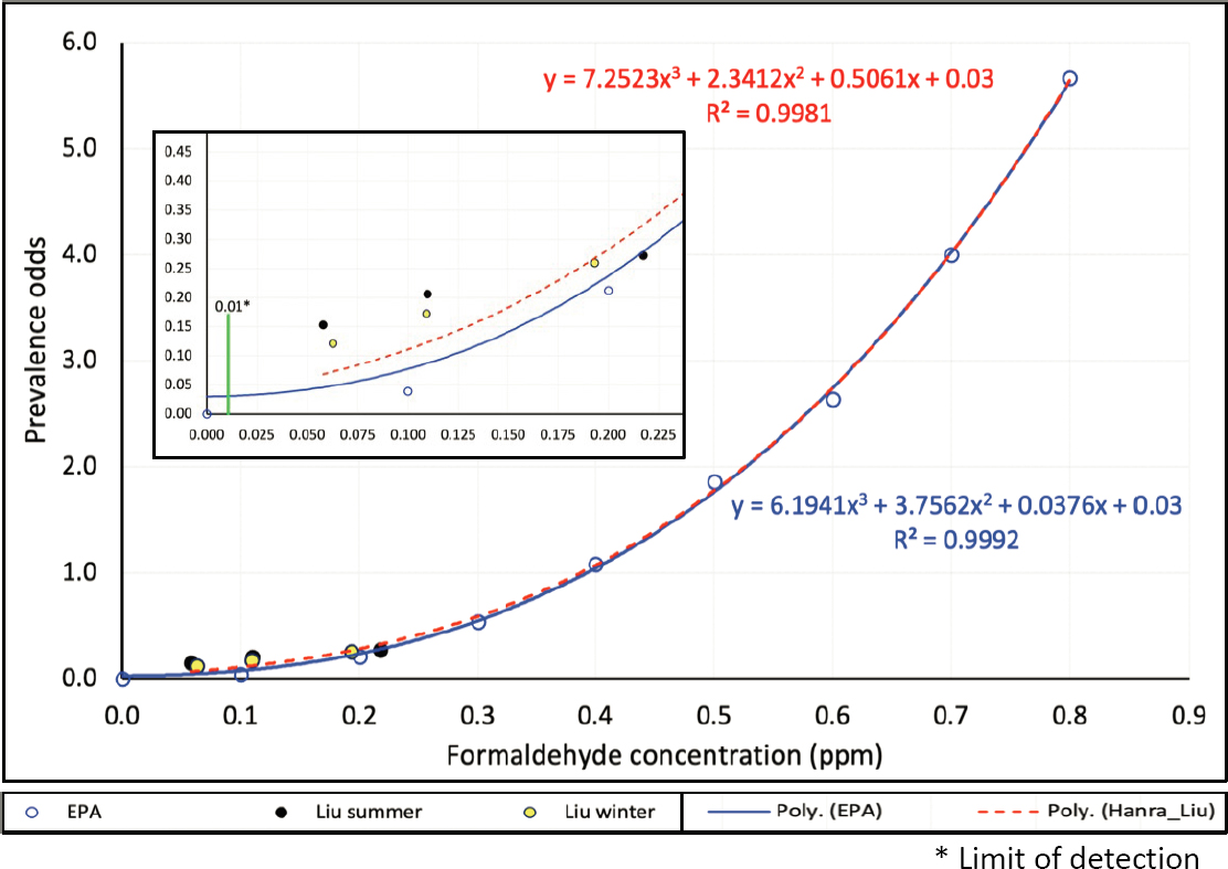
Hanrahan et al. (1984) used logistic regression analysis to estimate potential symptom risk ratio dependency upon respondents’ age, smoking status, gender, and the formaldehyde concentration measured in the home. EPA used data from Figure 1 in the Hanrahan et al. (1984) study to estimate the prevalence odds for corresponding formaldehyde concentrations. A third-order polynomial function was used to obtain the best-fitting curve (see Equation 1). An intercept of 0.03 was inputted into the model to represent a 3% background prevalence of sensory irritation. The third-order polynomial function was used to estimate formaldehyde concentration (exposure) that would increase the background prevalence by 10%. The corresponding prevalence odds that would generate a 10% risk difference was estimated to be 0.145. Equating the prevalence odds of 0.145
in Equation 1, where x represents formaldehyde exposure, EPA obtained a benchmark concentration (BMC10) of 0.153 ppm (= 0.188 mg/m3 at 25 ℃).
log odds = 0.145
= 6.1949 × x3 + 3.7689 × x2 + 0.0309 × x + 0.03 … … … … Equation 1
Step 2: Generation of the Exposure Distribution for Liu et al. (1991) from the Sexton et al. (1986)
Figure 1 in Liu et al. (1991) reports the percentages of respondents with burning eyes for three time-weighted exposure categories, by season. As these time-weighted exposure categories cannot be used to apply the same methods that EPA used for the Hanrahan et al. (1984) study (unweighted exposures), the committee used the exposure distribution presented in Figure 3 in Sexton et al. (1986). Figure 3 in Sexton et al. (1986) reports exposure for the same group of respondents as in the Liu et al. (1991) study. WebPlotDigitizer (Rohatgi, 2022) was used to generate the metadata from the histograms presented in Figure 3 from Sexton et al. (1986). The original histograms alongside the recreated graphs are shown in Figure D-2.
SOURCES: Hanrahan et al., 1984; Liu et al., 1991.
From the recreated plots, we assigned the proportion of the total respondents in Liu et al. (1991) to the respective exposure bins (Figure D-1, left panels). We estimated population weighted exposure for each bin, separately for summer and winter. The recreated residential indoor formaldehyde concentration distribution, shown in Table D-1, is supported by published data from Table 1 in Liu et al. (1991).
TABLE D-1 Comparison of the Exposure Categories Recreated from the Graph with Published Data from Liu et al. (1991)
| Indoor Concentrations | Data from the Recreated Histograms (%) | Published Data from Liu et al. (%) |
|---|---|---|
| Summer | ||
| <0.05 ppm | 30.1 | 30.8 |
| 0.05–0.1 ppm | 38.9 | 39.7 |
| >0.1 ppm | 31.0 | 29.5 |
| Winter | ||
| <0.05 ppm | 20.5 | 20.4 |
| 0.05–0.1 ppm | 48.0 | 49.6 |
| >0.1 ppm | 31.5 | 30.0 |
SOURCE: Based on data from Liu et al., 1991.
The numbers of mobile homes included in the study were 663 and 523, and the numbers of participants in the 20–64 age group were 739 and 587, in summer and winter, respectively. The committee used the 20–64 age group because the prevalence of eye irritation in Liu et al. was presented for this age group (see Figure 1 in Liu et al., 1991).
Hanrahan et al. (1984) presents unweighted exposure estimates. For Liu et al. (1991), the committee used weekly average indoor concentrations. To do that, we assumed that the distribution of the weekly average indoor formaldehyde concentrations in the mobile homes approximates the distribution of the time-weighted individual exposures in the Liu et al. (1991) study. This assumption is partially supported by an observation made by Liu et al. (1991), “For a person who spends 60% of the time inside his or her home, a weekly average HCHO [formaldehyde] exposure of 7 ppm-hr can be translated into a weekly average HCHO concentration of 0.07 ppm” (p.94). EPA made a similar assumption while comparing the benchmark concentration lower bound (BMCL10) obtained from the Hanrahan et al. (1984) study with that of the Liu et al. (1991) study (page 2-8, lines 14–17, main document).
Step 3: Modeling the Polynomial Function Using Data from Liu et al. (1991) and Hanrahan et al. (1984)
The committee used three data points for the prevalence of sensory irritation in summer (black circle) and three data points for winter (yellow circle), as shown in Figure D-1. The percentages were obtained from Figure 1 in Liu et al. (1991) and plotted against the unweighted indoor concentration exposure scale to make them consistent across the two studies. As the indoor concentrations within each category are within a relatively narrow range, we used the midpoint (population-weighted arithmetic mean) of the category to plot the prevalence from Liu et al. (1991).
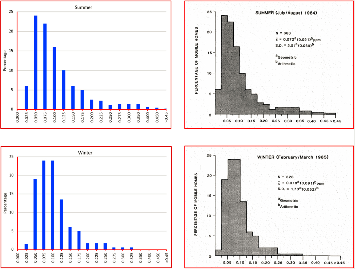
SOURCE: Based on data from Sexton et al., 1986.
Next we fit a similar third-order polynomial function using a fixed intercept of 0.03 to represent a 3% background risk. The curve representing the polynomial plot is shown by the broken red line in Figure D-1. The mathematical function is shown in Equation 2 below, where x represents formaldehyde concentration.
log odds = 0.145
= 7.2544 × x3 + 2.3384 × x2 + 0.507 × x + 0.03 … … … … Equation 2
The BMC10 value obtained from the new function developed using both Hanrahan et al. (1984) and Liu et al. (1991) is 0.1256 ppm (= 0.1542 mg/m3 at 25 ℃), as shown in Table 2. Continuing to replicate EPA’s methods, we estimated the BMC10 values by varying the background prevalence of sensory irritation to 2%, 1%, and 0% (see Table D-2).
TABLE D-2 Comparison of BMC10 Values Using Different Background Prevalences Generated Using EPA’s Methods, Hanrahan et al. (1984), and Liu et al. (1991)
| Background Prevalence | BMC10 (EPA; Hanrahan only), ppm (mg/m3) | BMC10 (Hanrahan + Liu), ppm (mg/m3) | Difference, ppm (mg/m3) |
|---|---|---|---|
| 3% | 0.1525 (0.1871) | 0.1256 (0.1542) | 0.0269 (0.0329) |
| 2% | 0.1531 (0.1879) | 0.1261 (0.1548) | 0.0270 (0.0331) |
| 1% | 0.1538 (0.1887) | 0.1266 (0.1553) | 0.0272 (0.0334) |
| 0% | 0.1544 (0.1895) | 0.1270 (0.1560) | 0.0274 (0.0335) |
NOTE: To convert ppm to mg/m3 we used values recommended by EPA. Molecular mass = 30.03 g/mol, molar volume = 24.45 L, and temperature = 25 ℃. BMC = benchmark concentration; EPA = US Environmental Protection Agency.
SOURCES: EPA 2022 Draft Formaldehyde Assessment; Hanrahan et al., 1984; Liu et al., 1991.
Findings: The BMC10 values estimated by EPA and those obtained by combining data from both studies are presented in Table D-2 and Figure D-1. Regardless of the background prevalence, the BMC10 values were consistently lower when data from both Hanrahan et al. (1984) and Liu et al. (1991) studies were used, compared with the values estimated using only the Hanrahan et al. (1984) study. The results also demonstrate that background prevalence does not substantially affect the BMC10 value.
COMPLEMENTARY CHARACTERISTICS OF HANRAHAN ET AL. (1984) AND LIU ET AL. (1991)
The two studies, Hanrahan et al. (1984) and Liu et al. (1991), share some key characteristics, which when considered together are likely to complement one another and strengthen the POD analysis:
- Indoor concentrations in Hanrahan et al. (1984) were estimated as the average of two samples (kitchen/living room and bedroom), with a range between <0.1 ppm and 0.8 ppm; the median was 0.16 ppm. About half of the indoor concentrations in Hanrahan et al. (1984) were between 0.1 and 0.16 ppm. Liu et al. (1991) measured indoor concentration over 7 days in the kitchen and bedroom. The values range between 0.01 (limitation of detection [LOD]) and 0.46 ppm with a geometric mean of 0.072 ppm for summer and between 0.17 and 0.314 ppm, with a geometric mean of 0.078 ppm, for winter.
- Although there is some overlap of concentrations between the two studies, Liu et al. (1991) indoor concentrations for two-thirds (68%) of the respondents were below 0.1 ppm, which is an approximate starting point of indoor concentrations in Hanrahan et al. (1984). The Hanrahan et al. (1984) study covers a wider range of exposure at the higher end (0.8 ppm), but data may be sparse at higher concentrations, given the median of 0.16 ppm and a total sample of 61 respondents.
- The Liu et al. (1991) study collected hours spent at home per day for the period of air sample collection, which allowed estimation of time-weighted exposure. However, these data cannot be combined with the Hanrahan et al. (1984) study data.
- The relevant sample in Liu et al. (1991) was about 10 times more than that in Hanrahan et al. (1984). More importantly, the prevalence of sensory irritation in Liu et al. (1991) covered an age group of 20–64 years. In comparison, Hanrahan et al. (1984) included teenagers and adults, but the prediction model that was used to derive the BMC is
- centered on the mean age of 48 years. In other words, although the model was developed using other ages, the predicted prevalence is for a population with a mean age of 48 years, somewhat limiting the generalizability.
LIMITATIONS
An important limitation of this case study is the unavailability of data, which led the committee to make an assumption about the exposure distribution in the Liu et al. (1991) study. Our finding of a lower BMC10 value when data points from both studies are used may not hold if the distribution of (unweighted) indoor concentrations differs markedly from the distribution of person–time exposure in Liu et al. (1991). Other limitations include the following:
- There is potential for selection bias in both studies.
- It is unclear whether Figure 1 in Liu et al. (1991) is based on predicted values from an adjusted model. In contrast, Hanrahan et al. (1984) estimates are adjusted for age and may also be adjusted for smoking and gender.
- In Hanrahan et al. (1984), mean (geometric) exposure for the respondents was reported to be 0.16 ppm (0.20 mg/m3), but 0.17 ppm (0.22 mg/m3) for nonrespondents (i.e., respondents were underexposed by 0.02 mg/m3).
Overall, the committee was able to replicate EPA’s methods. BMC10 values can be obtained by analyzing data from complementary studies that share some key characteristics.
REFERENCES
EPA (U.S. Environmental Protection Agency). 2022. IRIS Toxicological Review of Formaldehyde-Inhalation, External Review Draft. Washington, DC. https://iris.epa.gov/Document/&deid=248150 (accessed September 18, 2023).
Hanrahan, L. P., K. A. Dally, H. A. Anderson, M. S. Kanarek, and J. Rankin. 1984. Formaldehyde vapor in mobile homes: A cross sectional survey of concentrations and irritant effects. American Journal of Public Health 74(9):1026–1027. https://doi.org/10.2105/ajph.74.9.1026.
Liu, K. S., F. Y. Huang, S. B. Hayward, J. Wesolowski, and K. Sexton. 1991. Irritant effects of formaldehyde exposure in mobile homes. Environmental Health Perspectives 94:91–94. https://doi.org/10.1289/ehp.94-1567965.
NRC (National Research Council). 2014. Review of EPA’s Integrated Risk Information System (IRIS) process. Washington, DC: The National Academies Press.
Rohatgi, A. 2022. WebPlotDigitizer user manual version 4.6. Pacifica, CA. http://arohatgi.info/WebPlotDigitizer/app.
Sexton, K., K. S. Liu, and M. X. Petreas. 1986. Formaldehyde concentrations inside private residences: A mail-out approach to indoor air monitoring. Journal of the Air Pollution Control Association 36(6):698–704. https://doi.org/10.1080/00022470.1986.10466104.


