Assessing Lifecycle and Human Costs of Bus Operator Workstation Design and Components (2024)
Chapter: 4 Bus Packaging Methods
CHAPTER 4
Bus Packaging Methods
The objective of this work is to study driving postures of U.S. bus operators and make design recommendations regarding bus cab layout. The various approaches to vehicle packaging each have advantages and disadvantages. One might be suitable for one scenario and inappropriate for another. When deciding which method to use, many factors need to be considered, including available data, cost, and fidelity of results. An appropriate approach should be able to provide results of sufficient accuracy within a reasonable budget and meet the project expectations.
Besides selecting an appropriate model, another challenge is understanding the bus operator population as a whole. The work requirements and other considerations make the demographics of U.S. bus operators unique from the general population. The differences can be reflected in descriptors such as gender ratio, race/ethnicity composition, and age distribution. This information is vital to good design for human variability practice since it defines some of the variability that must be considered in the creation of the artifact, task, or environment. A poorly defined user population can result in designs that don’t meet accommodation expectations. This is especially problematic with designs like bus operator workstations, where adjustability is used to improve overall accommodation rates. Improperly allocated adjustability increases costs without improving performance.
The first half of this chapter discusses the approach used in this work and presents the models to predict driver posture. The second half of this chapter presents the demographics of U.S. bus drivers.
4.1 Model Selection
Vehicle packaging considers the spatial placement of components including displays, controls, and the seat. Recommendations should consider the driver population and the postures they are likely to prefer or exhibit while driving. These behaviors are a compound result of body dimensions and postural preferences. A successful package provides sufficient adjustability to accommodate a large fraction of these individuals and postures while minimizing the associated costs.
This research results in a toolkit to accurately predict the postures and associated joint center locations of populations of U.S. bus operators in response to a candidate cab geometry. The tool reports what fraction of operators in the specified population are capable of reaching the steering wheel and the pedals without any difficulty while simultaneously maintaining the ability to see target locations. Cascading posture prediction was selected for a number of reasons, including the experimental validation and its ability to conduct simultaneous multivariate prediction.
The toolkit provides numeric/tabular results as well as visual ones. Research has shown that including visuals can increase an individual’s patience in learning and understanding (81). Additionally, on average, 83% of what a person learns is through sight (82). Therefore, it would significantly reduce the learning curve associated with this new toolkit to include a visual representation
of the accommodation results. To be specific, the toolkit should clearly and accurately identify the critical landmarks (preferred steering wheel location, H-point location, and eye location), and accurately display the rest of the landmarks (shoulder location, elbow location, knee location, and ankle location).
As mentioned previously, industry users currently rely heavily on the SAE J tools and conduct mostly univariate analyses by designing interior components independently. The J tools provide sufficient information on how people react to each design objective and estimate how a driver’s interaction varies within a certain population, but they cannot provide a coherent understanding of how individuals adapt to several spatial requirements simultaneously. The correlation between the requirements is disjointed, especially from an individual level. More importantly, the SAE J tools are incapable of predicting postural adjustments due to disaccommodation. In other words, they provide information on the preferred location for a control, but not on what a driver might do when that preferred location is unattainable.
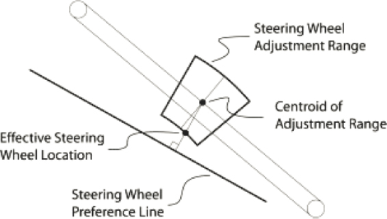
Current industry standards describe driver posture by estimating the distribution of the preferred locations of each landmark, such as steering wheel, H-point, and eye location. Assuming these are normally distributed, they can be represented with a mean and standard deviation. The advantage of such an approach is that distributions are continuous. Without needing an infinite number of drivers, it produces results of infinite resolution. The disadvantages are apparent as well. The main issue is the model cannot adjust based on bus geometric constraints, because the underlying relationship between meeting multiple design objectives remains uncertain. While designing an adjustment envelope for the steering wheel, for instance, a high accommodation rate is desired, but disaccommodated drivers are expected as well. When a driver’s preferred steering wheel location is not in the adjustment envelope, they will move the steering wheel to the nearest point on the envelope and adjust the rest of their body to accommodate this change (Figure 4.1) (37).
The purpose of a new design is to minimize these required changes to a driver’s preferred posture. In order to visually reflect how adjusting one landmark can impact the location of other landmarks for every virtual bus operator, it is important to approach vehicle packaging from an individual perspective. That is the strength of the VFT approach—each virtual driver is allowed to interact with the candidate design individually and their responses are predicted. Then the individual results are aggregated to predict behavior for an entire population. This mirrors what would happen in a real usage scenario.
Overall, the model needs to be able to (1) predict locations of critical landmarks with high accuracy, (2) assess design objectives using a multivariate approach, and (3) use visuals to present packaging results. Considering all the available approaches discussed in Chapter 2, the first two needs can be met using cascade modeling, and data visualization can be achieved through virtual fitting.
4.2 Cascade Model for Buses
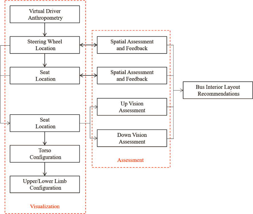
Previous research has laid a foundation in Class B vehicle packaging, and a cascade model for buses and trucks was developed in 2005. Its core concepts can be summarized in a flowchart (Figure 4.2). This section details the cascading procedure of driving posture prediction.
4.2.1 Steering Wheel Location
In posture prediction, identifying the preferred steering wheel location is one of the first steps. Most vehicles now include adjustable steering wheels. Due to the spatial demand of the operator cabs among large vehicles, especially buses and trucks, steering wheels need to provide suitable adjustment ranges for drivers to maintain sufficient vision while driving. There are two common modes of adjustment: tilting and telescoping. Tilting is when a steering wheel rotates about its pivot point, located at the base of the steering wheel. Telescoping is when a steering wheel moves parallel to the shaft (Figure 4.1). With the two modes of adjustment, the steering wheel can move in both X and Z directions.
Drivers tend to place the steering wheel at the most comfortable location for them to perform normal driving tasks. Preferred steering wheel locations vary from person to person, which makes it challenging to predict driver preference. In an attempt to understand such variability, a laboratory study was conducted to investigate preferred steering wheel location for vehicle operators. Participants were asked to sit in a simulated cab and adjust the floor height and the pedals in the X (fore-aft) and Z (vertical) directions. Instead of the steering wheel, the origin of the cab (AHP) was adjusted because steering wheels were fixed in space in the experiment setup. This allowed the relative location between the steering wheel and the pedals to vary based on driver preference. After each driver adjusted to their preferred posture, data were collected (37).
The preferred steering wheel location data (measured from the AHP) indicated that the vertical location of the steering wheel is negatively impacted by its horizontal location, and a near-linear relationship was discovered. The average ratio (mean) was calculated to be −0.559 with a standard deviation (SD) of 0.305. In other words, the vertical location is expected to decrease by an average of 0.559 mm for every 1 mm the steering wheel travels back horizontally. And 67% of the drivers will likely choose a ratio between −0.864 p (Mean − SD) and −0.254 p (Mean + SD).
| SWprefz - 0.559 * SWprefx | (4.1) |
where SWprefz is the steering wheel preference Z coordinate and SWprefx is the steering wheel preference X coordinate.
The variance of the ratio was also derived from the driver’s preference, and it was independent of driver anthropometry (37). However, the preferred total height of the steering wheel is strongly dependent on the driver’s stature (height). Stature is a widely available anthropometric measure and a common predictor in postural models, including in vehicle packaging. The preferred vertical location is found to be
| SWprefz@175(mm) = 524 + 0.1613 * stature, R2 = 0.32, RMSE = 23.4 | (4.2) |
when the horizontal location is at 175 mm with respect to the AHP. The horizontal location of 175 mm does not hold actual meaning and is chosen merely for mathematical convenience. In fact, any horizontal location can be chosen because the preferred vertical locations move along a slope of 0.559, as mentioned. These preferred vertical locations can be found by using the equation:
| SWprefz(mm) = 524 + 0.1613 * stature - 0.559 * (x - 175) | (4.3) |
This line represents the steering wheel preferred vertical locations. Based on their stature, each driver has a unique preferred steering wheel vertical height line (Figure 4.1).
One preference line is not enough to locate a preferred steering wheel location in a 2D space because there are two degrees of freedom (DoF); a minimum of two lines are needed. Besides steering wheel vertical height, human variability can also be reflected in the steering wheel tilt angle. Rotating the steering wheel about the pivot point not only allows drivers to control the face angle of the steering wheel so it is easier to grab, but also enables the steering wheel to move in the horizontal direction to adapt fore-aft preference. By drawing a line connecting the steering wheel pivot of rotation to the center of the steering wheel, a driver’s preferred tilt angle can be found. These two lines can be used to find the intersection that represents the driver’s preferred steering wheel location (37).
For a properly designed vehicle, the majority of preferred steering wheel locations should be accommodated. In fact, the adjustment envelope should be selected after the preferred locations are found. Once the envelope is determined, it can be used to locate the fore-aft and vertical locations of the center of the steering wheel with respect to the AHP, which are to be used as
inputs for the rest of the posture prediction. If the preferred location lies outside the adjustment envelope, the nearest point to the envelope is used (37). Specifically, two measures need to be assessed: tilt angle and telescope distance. Both need to be within the vehicle adjustment range. If one exceeds that range, the most extreme location in the range will be selected (Figure 4.3).
This model provides a mathematical understanding of how drivers would adjust the steering wheel to a preferred location based on their body dimensions and their driving preference. It was developed using laboratory data and has been verified in the field.
4.2.2 H-Point Location
The seat is another adjustable component inside a vehicle. Its location is usually defined by the H-point, which generally represents where a driver’s hips would be. One of the design concerns of seat location is that drivers must be able to comfortably reach the pedals with their feet. This is a fundamental requirement of vehicle packaging and an indicator of spatial accommodation. Another concern of locating the driver’s H-point is to provide reasonable relative location between the hand grip and the torso. Similar to reaching the pedals with the feet, reaching the steering wheel with the hands is important. Once the steering wheel location and the seat location are chosen, driver eye location will be assessed for safety considerations. A more detailed discussion on driver field of view is presented in section 4.2.3.
The cascade model used for some of the posture prediction was developed based on linear regression, in the form of constant coefficients multiplying predictors (c).
| y = c0 + c1 * x1 + c2 * x2 . . . | (4.4) |
Here, y represents the dependent variable, which is the variable of interest. The independent variables (x1, x2, etc.) are predictors. In vehicle packaging, two kinds of predictors are common: driver anthropometry and vehicle geometry. Driver anthropometry describes body size and
shape and plays a major role in spatial fitting, which mostly determines body landmark locations. Vehicle geometry also contributes to the effect because drivers commonly adjust their posture to adapt to the vehicle’s interior component layout. Taking these two predictors into account allows for accurate prediction of the average location of a desired landmark.
This linear regression is useful for predicting drivers’ average behavior but is insufficient to express the ranges of individual preference uncorrelated with anthropometry that most drivers exhibit. To include this factor, the residual variance from the regression model is reintroduced into the equation (43). The error term N (0, s) is a randomly generated number from a Gaussian distribution. This distribution has a mean of zero and a standard deviation of s, the square root of the residual variance. By studying the size of the error and augmenting this error to the linear regression, a complete spectrum of driver preference can be captured through this model.
| y = c0 + c1 * x1 + c2 * x2 . . . + N(0, s) | (4.5) |
As discussed in Chapter 2, an H-point is a fixed point on a car seat near the driver’s hip. Unlike a hip point that moves with the driver’s posture, an H-point is a characteristic of the seat. Given an H-point location with respect to the AHP, it’s possible to accurately locate the seat. One of the objectives of vehicle packaging is to design a proper seat adjustment envelope (the region the H-point can move through). Thus the H-point, instead of the hip point, is commonly used.
The H-point can be measured on a physical seat using an H-point machine and the procedures outlined in SAE J826 (42). Researchers have also created a linear regression model that can predict the preferred H-point location of a population with high accuracy (37). One of the factors that led to its success is that it uses a stepwise approach in an iterative manner (83). For instance, there are a number of anthropometric measurements that are related to the length of a human body, including stature, leg length, arm length, erect sitting height, and acromial height. This introduces more predictors than needed and can lead to more errors because certain body characteristics are overanalyzed. A stepwise approach carries out an automatic process of choosing predictors to fit regression models. During each step, one predictor is analyzed to determine whether to add it to or subtract it from the current list of predictors.
Through an iterative stepwise approach, two predictors regarding vehicle geometry (fore-aft and vertical locations of the center of the steering wheel with respect to AHP) and five predictors regarding anthropometric measurements (stature, erect sitting height, ratio of erect sitting height to stature, difference between stature and erect sitting height, and natural log of body mass index [BMI]) were identified (37). Since anthropometric measurements are approximately normally distributed, each measurement of a population can be represented with a mean and a standard deviation. The stepwise regression results indicate that the horizontal location of the H-point is largely dependent on the horizontal and vertical location of the steering wheel, which is a sign of drivers adjusting their seating to adapt to vehicle interior components. For this reason, steering wheel location is predicted first and is used as inputs for seat location prediction, although drivers usually adjust both of them simultaneously in an iterative manner. The driver’s functional leg length is estimated by taking the difference between stature and erect sitting height. A positive coefficient shows that drivers with longer legs tend to adjust the seats backward.
BMI is the other predictor that indicates body width. Usually, a wider driver would need more space to operate a vehicle. The purpose of using the natural log is to normalize the BMI measurements of the population, which otherwise exhibit a long right tail. The standard deviation of the error term is 37.7 mm, which represents a driver’s postural preference unrelated to anthropometry (37).
| Hx(mm) = -53.6 + 0.6081 * SWpivot x - 0.3343 * SWpivot z + 0.6394 * lleg + 89.07 * Ln(BMI) + N(0, 37.7) | (4.6) |
where
| Hx = | H-point location X coordinate |
| SWpivotx = | steering wheel pivot point X coordinate |
| SWpivotz = | steering wheel pivot point Z coordinate |
| lleg = | functional leg length |
| Ln(BMI) = | natural log of BMI |
Unlike the horizontal location, which uses four predictors, the vertical location of the H-point is dependent solely on the vertical location of the steering wheel. Anthropometric measurements regarding body length or width had a minimal effect. The standard deviation of a driver’s preferred seat vertical location is 22.9 mm, which is smaller than horizontal (37).
| Hz = -200.3 + 0.8545 * SWpivot z + N(0, 22.9) | (4.7) |
where Hz is the H-point location Z coordinate.
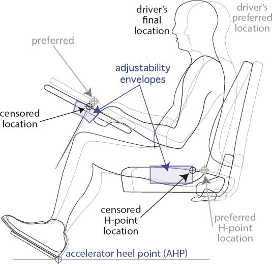
While designing a seat adjustment envelope for the preferred seat location of a driver population, the huge amount of potential variability makes it impossible to accommodate 100% of them. Consequently, the accommodation goal is commonly set at 95% or lower for economic and/or practical reasons. For virtual drivers who are accommodated by the candidate design (i.e., they can put the seat in their preferred location), the cascade posture prediction model will proceed to the next step. For the disaccommodated virtual driver, the predicted location becomes the nearest point on the adjustability envelope to the preferred location. Then their posture is adjusted accordingly (37).
4.2.3 Eye Location
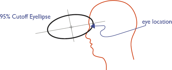
The cascade model received its name from its cascading nature; a sequence of actions must take place in order to achieve the desired goal. The first step is to predict the virtual driver’s preferred steering wheel location. After this, seat location can be predicted. The cascade model can then proceed to estimate the driver’s eye location. In vehicle packaging, the location of the eye center is represented by the eye point (Figure 4.4). The range of eye locations in the 2D X-Z plane for a population of drivers is referred to as the eyellipse. Generally, the movement limits are 45° upward, 65° downward, and 30° left and right, but for comfort, a 15° turn in all four directions is considered “easy eye rotation” (29). In SAE J1050, the eye point is defined in 3D space with the left and right eyes fixed 65 mm apart. Since this work studies vehicle packaging in the 2D X-Z plane, only the eye point on the X-Z plane is calculated and used for performance assessment.
In the referenced cascade model, the eye point was studied in a similar manner as the H-point, through laboratory data, and the same set of predictors are used. Both steering wheel location
and seat location are predicted from the AHP, the origin of vehicle interior component packaging. However, the eye point location developed in this model is expressed relative to a different datum. Due to the limited movement of the driver’s neck during driving, the driver’s head and torso are relatively static. In other words, the driver’s eye point is largely dependent on the seat location, so eye points are expressed in terms of H-point (37). In the horizontal direction, the eye point is found to be a function of three predictors: the horizontal location of the steering wheel, the ratio of sitting height to stature, and BMI. This regression model (Equation 4.8) also incorporates a residual variance term that represents preference unrelated to anthropometry. The square root of the residual variance was found experimentally to be 41.0 mm. In the vertical direction, the eye point (Equation 4.9) is a function of only one predictor, erect sitting height, and has s = 22.3 mm (37).
| Eye x = -334.0 + 0.0809 * SWpivot x + 1142 * ratio - 87.98 * Ln(BMI) + N(0, 41.0) | (4.8) |
where Eyex is the eye point X coordinate.
| Eye z = -47.3 + 0.7812 * SittingHeight + N(0, 22.3) | (4.9) |
where Eyez is the eye point Z coordinate and SittingHeight is the driver’s sitting height.
Driving requires a number of actions that involve the steering wheel, foot pedals, buttons, and other interior components. These actions are essential to operating a vehicle as desired, but the ability to see outside of the vehicle is even more important because the driver’s sight is the main source of information they use to make decisions. The central vision field, straight through the front windshield, allows drivers to see cars, pedestrians, traffic lights, and signs in the front. Besides central vision, peripheral vision is also important because it captures cars and other potential hazards. The quality of driver vision can directly impact driver safety and performance (84). Since this work is conducted only in the X-Z plane, only central vision is considered.
A driver’s central vision in two dimensions is bounded by the driver’s ability to look both upward and downward. Upvision angle is measured from the horizontal plane to the highest angle the driver can see, and downvision angle is measured to the lowest angle. The sum of the two angles makes up the driver’s central vision. In most vehicles, the upvision angle is limited by the UDLO, where the top of the windshield meets the frame of the vehicle. An adequate upvision angle permits the driver to read road signs, respond to traffic lights, and see traffic on uneven roads. According to the American Public Transportation Association (APTA) bus design guideline, the windshield must ensure a minimum of a 14° upvision angle (8).
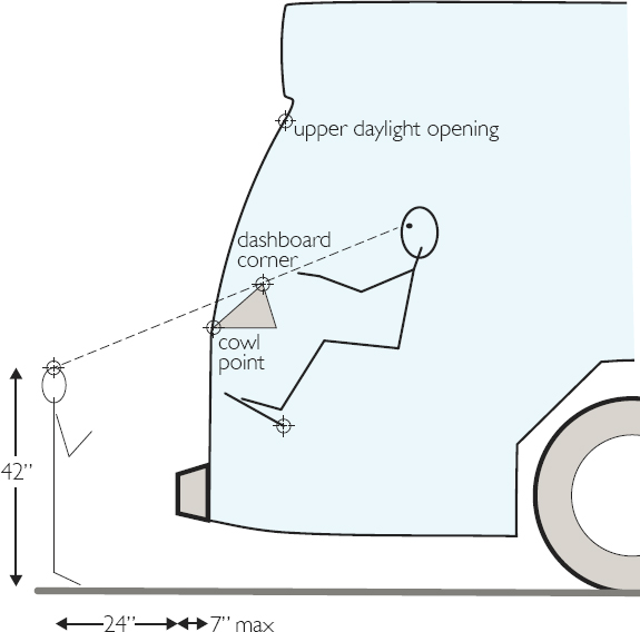
Downvision is also important, particularly because buses are typically higher than the vehicles around them. This makes it challenging for drivers to see immediately in front of the bus. This issue is especially profound in urban areas where traffic and pedestrians are primary concerns. Additionally, school transportation is one of the main ways buses are used, where picking up and dropping off children is the most essential part of the job. Bus drivers must be able to maintain adequate downward vision to ensure clearance in front of the bus. Thus, APTA requires all bus drivers to detect an object 42″ high and 24″ in front of the bus (Figure 4.5). These upvision and downvision requirements agree with SAE practice (29), and they are used as design guidelines in this work.
Upvision is usually defined by the location of the UDLO, but downvision requires more consideration. Depending on the geometric layout, a few interior components could be the limiting factor. The most common consideration is the location of the cowl point—where the bottom of the windshield meets the body of the bus. If it was designed to be above the line connecting the driver’s eye point and the tip of the 42″ object, the requirement would be unmet. Besides the
cowl point, some buses are equipped with a hood. The hood point, which represents the highest point on the front end of the hood, can also be a limiting factor. Another candidate is the dashboard. As more functionalities are added to buses, the dashboard is growing bigger to fit an increased number of buttons and screens. As designers assess a bus package, all the potential obstacles need to be considered to ensure a safe downvision angle.
4.2.4 Secondary Body Landmarks
The purpose of vehicle packaging is to apply an understanding of drivers’ behavior inside a vehicle and make design decisions on the layout of the interior components to best accommodate them. In this work, most of the essential components in the X-Z plane are included: steering wheel, seat, and vision-related components. They are assessed with drivers’ preferred steering wheel location, H-point, and eye point. This knowledge allows for successfully packaging many elements of a bus layout. As discussed at the beginning of this chapter, besides accurately predicting drivers’ postures, visually representing these postures is significantly useful for industry users. This section briefly discusses how secondary body landmarks (hip point, shoulder point, grip point, elbow point, ankle point, and knee point) are predicted.
In the study of biomechanics, a human body can be presented using body landmarks. In vehicle packaging this is often accomplished through representations of the body as body segments and joints (85, 86, 87). This approach not only gives a visual representation of the drivers but also works seamlessly with the cascade model. As a continuation of the cascade model, the next step is to use inverse kinematics to estimate the locations of other body landmarks, which is useful to assess accommodation and visualize the driver.
In previous sections, linear models of finding the preferred H-point were presented. The H-point is a fixed location on a seat and does not move relative to the seat based on driver
preference. A hip point, however, is the joint center of a driver’s hip. It is a commonly used body landmark when configuring driver posture since it is part of the kinematic chain connecting the upper and lower body segments.
The location of the hip for each virtual driver can be estimated using linear regression. The offset vector from the H-point to the hip point is a function of the driver’s body dimensions (37). Specifically, the horizontal offset distance is negatively proportional to the driver’s BMI, and the vertical offset distance is positively proportional to both the driver’s BMI and erect sitting height. By adding these offset distances to the H-point location, the hip point location can be found. Since the following body landmarks are mainly used for visualization and have minimal impact on vehicle interior layout, simple linear regression models are used without variance. Hip point location is calculated as follows:
| Hip x = 90.2 - 5.27 * BMI + Hx | (4.10) |
| Hip z = -109.9 + 1.51 * BMI + 0.0813 * SittingHeight + Hz | (4.11) |
where Hipx is the hip point X coordinate and Hipz is the hip point Z coordinate.
For consistency of terminology, the shoulder joint center, elbow joint center, and knee joint center are referred to in this report as the shoulder point, elbow point, and knee point. Once the hip point is located, the next joint center in the kinematic chain—the shoulder—can be predicted. While driving, the shoulder point and hip point together represent the driver’s torso. Commonly, drivers lean their torso against the back of the seat to reduce stress. Taking this slouching factor into consideration, researchers have found the distance between the hip point and the shoulder point to be a function of the driver’s erect sitting height. As Equation 4.12 indicates, the distance is solely impacted by the driver’s length. However, the angle between the two is largely dependent on the driver’s width (Equation 4.13). This angle (measured from the vertical direction) can be predicted:
| HipShoulderDist = 0.49 * SittingHeight | (4.12) |
| HipShoulderAngle = -25.1 + 0.297 * BMI + 67.6 * ratio | (4.13) |
where the distance (HipShoulderDist) and angle (HipShoulderAngle) between the two points, the X- and Z-offsets, can be calculated using trigonometry. The location of the shoulder point can be obtained by augmenting the offsets to the hip location:
| Shoulderx = Hip x + HipShoulderDist * sin(HipShoulderAngle) | (4.14) |
| Shoulderz = Hip z + HipShoulderDist * cos(HipShoulderAngle) | (4.15) |
where Shoulderx is the shoulder joint center X coordinate and Shoulderz is the shoulder joint center Z coordinate.
The next step is locating the center of the steering wheel. The preferred steering wheel angle was also calculated, measured from the vertical direction by convention. This angle is the same as the angle formed between the wheel face and the horizontal direction. Knowing the steering wheel diameter (SWD), once again, the X- and Z-offsets can be found using trigonometry and can then be added to the steering wheel location, which indicates the driver’s grip point.
| Grip x = SWx + SWD/4 * cos(SW angle) | (4.16) |
| Grip z = SWz - SWD/4 * sin(SW angle) | (4.17) |
where
| Gripx = | grip point X coordinate |
| Gripz = | grip point Z coordinate |
| SWD = | steering wheel diameter |
| SW angle = | preferred steering wheel angle |
The grip point, the shoulder point, and the elbow point form a triangle. With two of the vertices and one side being known, the third vertex can be positioned by knowing the lengths of the other two sides. One of the sides is the upper arm length, which is measured from the shoulder center joint to the elbow center joint, and this length can be estimated using the acromial radial length from an anthropometry database, such as the second U.S. Army Anthropometric Survey (ANSUR II) (9) which is discussed in section 4.3.1. In the survey, distances are measured from landmarks to landmarks, such as the acromion and the radial. Although these landmarks are different from the joint centers, researchers have quantified the offsets between them (88). Likewise, the length between the elbow joint center and the grip center can be estimated to represent forearm length. After knowing both upper arm length and forearm length, the elbow joint center can be estimated.
Due to the similarities between the upper limbs and the lower limbs, the same trigonometric procedure can be applied to lower-body configuration. Instead of the grip point, an ankle joint center is used. Relative to the AHP, researchers estimated the ankle to be 32 mm in the X direction and 128 mm in the Z direction (89). This is approximated as a constant since there is relatively little variation from the base of the heel to the malleolus landmark across individuals. Besides the ankle point, leg lengths are needed. One of them is the thigh length, which represents the distance between the hip joint center and the knee joint center. The other is the shank length, which represents the distance between the knee joint center and the ankle joint center. After knowing the lengths and locations of two vertices, the third vertex can be configured using the fundamentals of trigonometry, which represents the knee joint center.
4.2.5 Estimation of Accommodation
The cascade model used in this project advocates the principle of letting information flow down from experts through layers of customized treatment to obtain desired outcomes (90). In vehicle packaging, the cascade model applies a similar concept. The driver’s anthropometric dimensions and vehicle geometry are the high-level data. With these data, preferred steering wheel location is predicted. Using preferred steering wheel location as an input, preferred seat location is then predicted. Although these two steps usually take place iteratively in a laboratory setting or in real life, they are carried out sequentially in the VFTs because the model was developed based on final locations of these reference points. From here, eye point is predicted and field of vision is assessed. Once these primary locations are predicted, secondary body landmarks can be estimated, starting with hip point and shoulder point. After this, grip point, ankle point, elbow point, and knee point can be calculated.
Throughout the process of cascade posture prediction, a total of four design objectives were assessed. They are (in order of prediction):
- Steering wheel adjustment envelope accommodation
- Seat adjustment envelope accommodation
- Upward vision (minimum of 14°)
- Downward vision (must see a 1,067-mm object 610 mm in front of the vehicle)
The multivariate approach of assessing the accommodation condition of each virtual driver is a significant component of this work. With a large population of drivers as inputs, it provides
high resolution and allows designers to study the aggregated effects of design decisions. For each driver, designers can directly assess how they are accommodated on each of the four objectives. This approach facilitates an understanding of the underlying relationship between the objectives. When calculating overall accommodation, which is the proportion of drivers who have met all four design objectives, an accurate result can be given. Otherwise, assumptions would need to be made on who is disaccommodated on more than one design objective.
Anthropometric accommodation is described as the proportion of intended users who are within the range of desired objectives (91). Frequently, a percentile method is only suitable for univariate accommodation models. With multiple objectives, adding and subtracting cannot accurately combine accommodation results (92). One common approach to assess multivariate accommodation is through the intersections of sets, because of the comparable nature of the two mechanisms (93). While performing set intersection, set correlation is considered. For a pair of positively related variables, the intersection can be calculated as:
| P(A + B) = rAB * (SD A * SD B) + P(A) * P(B) | (4.18) |
where rAB is the correlation between the two variables, and SDA and SDB are the standard deviations. For negatively related (disjoint) variables, the correlation is zero, which simplifies the calculation to:
| P(A + B) = P(A) * P(B) | (4.19) |
Intersection of sets is a well-known method and has been validated with simulation data (93). However, the effort of studying variable correlations is costly. Since this work conducts design assessments for each individual in the population, a sequence of true/false indicators can be assigned to them instead. The outcome of assessing each design objective is either true or false. For such binary assessment, an indicator function assigns a value of 0 or 1 to each event based on the accommodation condition (93). In this work, a total of four design objectives were assessed, so each virtual driver was assigned four binary digits to indicate their accommodation. For instance, if the indicator functions generate 1-1-1-1 for a driver, the driver is expected to be accommodated on all four objectives. Similarly, a 1-1-1-0 indicates that the driver failed the downward vision requirement (the fourth test) but is accommodated on all others.
4.3 Bus Driver Population
The cascade model used in this work passes information through a sequence of models. The outputs from the previous model become the inputs to the next model. To improve the reliability of the final results, users can (1) choose the most appropriate model and (2) increase the fidelity of the inputs, namely vehicle geometry and driver population anthropometry. This section discusses the U.S. bus driver population and the available information that can be used in this work.
4.3.1 Anthropometric Database
Conventionally, military studies are the main source of anthropometric data for many design references and standards. Due to the large quantity of reported measures and rigorous methods of data collection, the 1988 U.S. Army Anthropometry Survey (ANSUR I) has been arguably the most frequently used anthropometric database globally. ANSUR I reported 132 directly measured dimensions and derived an additional 60 dimensions from each of the 3,982 U.S. military personnel (1,774 men and 2,208 women). It also included the demographic information, such as age, race, and ethnicity, to make it possible to sample from the most appropriate population (94). However, this does not represent the general U.S. civilian population well, especially
for dimensional extremities. For instance, obesity is underrepresented in the military. Because of the military’s strict selection requirements, ANSUR I and II data reflect a young, healthy, and athletic population. If a design for the civilian population uses ANSUR I or II data to simulate user interaction, the result will not be reliable (95).
Over time, secular trends in increased body size made the ANSUR I data inappropriate for even military use and a follow-up study was conducted in 2012. This used a broader sampling strategy and added whole-body scans. ANSUR II collected measurements from a total of 6,068 participants (4,082 men and 1,986 women), including reservists, and found that weight, circumferences, and breadths had all increased. It also found that the variation in these measurements had increased (Figure 4.6). ANSUR II replaced ANSUR I and was made publicly available in 2017 (9). Even though it is not an explicitly accurate approximation of the U.S. civilian population, it still contains useful information and can be used in the early phases of research.
The results from ANSUR II reflected that secular trends over the previous 30 years are noticeable and significant. Unlike ANSUR I and II, the National Health and Nutrition Examination Survey (NHANES) has been conducted continuously in the United States since 1999 (96). This sampling method makes it a suitable tool to analyze demographic trends in civilian populations. The most important observation is that mean mass (body weight) and BMI have both have been increasing, especially weight, which agrees with ANSUR II (97). One of the biggest advantages of NHANES is the oversampling strategy. By oversampling the tails of the anthropometric distribution, the underrepresented groups are included at a higher frequency, which ensures that there are plenty of data in these groups. Thus, each measured individual has an associated weight that indicates the size of the population they represent. In the 1980s, UMTRI designed manikins of various sizes by combining NHANES anthropometric data and stereophotogrammetry. This knowledge was then applied in automobile design (98, 99, 100). One distinct disadvantage of the NHANES data is that they only collect a limited number of measurements, such as stature, mass, and BMI. However, data synthesis methods (101, 102, 103) can be used to estimate the desired body dimensions through known relationships in more detailed datasets like ANSUR II. Once the appropriate detailed U.S. bus driver anthropometry data are available, they can be used as inputs to the cascade model.
4.3.2 Bus Driver Demographics
The four main types of bus drivers in the United States are school bus drivers, local transit bus drivers, intercity bus drivers, and charter bus drivers. Data from the Bureau of Labor Statistics show that in 2018, among all 681,400 bus driver jobs, 497,500 (73%) were provided by schools and special clients. Transit and intercity bus drivers held about 183,800 (27%) of jobs (Table 4.1).
Table 4.1. Industry composition of U.S. bus drivers in 2018.
| Type | Count | Percentage |
|---|---|---|
| School and client | 497,500 | 73.01% |
| Intercity and transit | 183,800 | 26.97% |
| Others | 100 | 0.015% |
| Total | 681,400 | 100% |
Many bus drivers operate through heavy traffic or bad weather, and sometimes deal with unruly passengers. Because of the road hazards and mental stress, bus drivers have one of the highest rates of injuries and illnesses of all occupations (104). Unlike many other jobs, bus drivers have a spatially limited workstation. While driving, they frequently maintain a driving posture for hours before taking a break. Thus, a well-designed bus cab can significantly improve the working conditions for a driver.
While designing a bus cab, proper driver demographics must be specified. Otherwise, the final design would be inappropriate and ineffective. In 1987, a study on urban transit buses used in Hong Kong discovered that many buses were designed based on European anthropometric data and were built in the United Kingdom. This resulted in bus workstations that were not suitable for the Cantonese workforce (105). This study showed that the designs for one racial or ethnic group do not necessarily accommodate another racial or ethnic group. This fact raises the challenge in the United States because the U.S. workforce has become more diverse not only in racial or ethnic composition, but also in gender composition, age, and other aspects. The next few sections report and discuss U.S. bus driver demographics, with the aim of understanding the driver population and providing important design guidelines.
4.3.3 Gender Composition
In the past several decades, many occupations have been dominated by either men or women. This was true especially before World War II. For instance, the secretarial workforce was almost exclusively women, and the commercial driver workforce was limited to men (106). However, the demographics have shifted in the United States in recent years. In 2020, the U.S. Department of Labor reported that women comprised 47% of the total U.S. labor force (107). This trend of improved participation of women is also present in the commercial driver workforce.
Despite earlier increases in participation from women in the commercial driver workforce, according to the American Community Survey (ACS) provided by the Census Bureau, the ratio of men to women has been consistent over the past few years (2014–2017). In 2018, men were 54.7% of the workforce to 45.3% women (108). As the years go by, a small fluctuation is observed in the total number of drivers and the gender composition, but overall they remain about the same (Table 4.2). Thus, this ratio should be used as the default for driver demographics, posture
Table 4.2. U.S. bus driver gender composition 2014–2017.
| Year | Men | Women | Total by Year | Percentage Men | Percentage Women |
|---|---|---|---|---|---|
| 2014 | 401,946 | 331,576 | 733,522 | 54.8% | 45.2% |
| 2015 | 424,168 | 347,898 | 772,066 | 54.9% | 45.1% |
| 2016 | 406,475 | 333,660 | 740,135 | 54.9% | 45.1% |
| 2017 | 393,972 | 334,603 | 728,575 | 54.1% | 45.9% |
| Total by Gender | 1,626,561 | 1,347,737 | 2,974,298 | — | — |
| Average | — | — | — | 54.7% | 45.3% |
prediction, and accommodation assessment. However, this ratio only represents the national average and could vary in different regions or due to specific driving responsibilities. To maintain reliability of the bus design, industry designers need to conduct driver demographics studies and modify the men-to-women ratio to best represent the driver population. More detailed information on gender composition can be found in Appendix B.
4.3.4 Race and Ethnicity
The United States is currently the third-largest country in the world by population and is known for its diversity. As of 2018, the White population constituted the majority at 76.4%, and the Black or African American population stood second at 13.4% (108). Such racial and ethnic composition is reflected in the employment market. In 2018, the White and Black or African American population made up 73.6% and 12.0% of total employment in the United States, respectively, which matches closely with the racial and ethnic composition of the population.
Similar to most other occupations, racial and ethnic diversity can be found in the bus driver workforce. ACS showed that the bus driver workforce consists of 62.9% White drivers, 27.7% Black or African American drivers, 2.2% Asian drivers, and 7.2% drivers of other races in 2017. Comparing the racial and ethnic composition of the bus driver workforce to that of the general U.S. workforce, the White population (62.9%) and the Black or African American population (27.7%) dominated with a total of 90.6% of the workforce, which is expected. This was found in previous years as well (Table 4.3). Detailed data of racial and ethnic composition in the bus driver workforce and the entire U.S. job market from 2014 to 2017 are in Appendix B. The percentage of White bus drivers fluctuated between 62.0% and 64.4%, and the percentage of Black or African American bus drivers fluctuated between 27.0% and 28.0% within these 4 years. This indicates that the relatively high prevalence of White and Black or African American drivers is likely to continue for the next several years.
The bus driving occupation is more common in some racial and ethnic groups than others. In 2017, 12.0% of the U.S. workforce was Black or African American employees, but 27.7% of bus drivers were Black or African American. Using racial and ethnic composition in general society as a reference, there were proportionally more Black or African American drivers than White drivers or Asian drivers by a large margin. This phenomenon exists in the previous 4 years as well (as shown in Appendix B). This is strong evidence that the proportion of Black or African American bus drivers in the workforce is about twice the proportion of Black or African American people in the U.S. workforce. Even though the previous observation shows that racial and ethnic diversity in bus drivers mostly match racial and ethnic diversity in the general population, proper adjustments still need to be made for more accurate simulation results.
4.3.5 Age
Besides the men-to-women ratio and racial and ethnic composition, age is another important descriptor of the U.S. bus driver demographics. Most states require their bus drivers to be at least
Table 4.3. U.S. bus driver ethnicity 2014–2017.
| Year | White | Black | Asian | Other |
|---|---|---|---|---|
| 2014 | 64.4% | 27.0% | 1.9% | 6.7% |
| 2015 | 63.1% | 27.5% | 2.3% | 7.1% |
| 2016 | 62.0% | 28.0% | 2.5% | 7.5% |
| 2017 | 62.9% | 27.7% | 2.2% | 7.2% |
| Average | 63.1% | 27.6% | 2.2% | 7.1% |
18 years old. Some require commercial drivers who drive across state lines to be 21 or older. A maximum age limit does not exist. Instead, interstate bus drivers must successfully complete a physical exam every 2 years, per federal regulations (108).
As discussed, men constitute 54% of the bus driver workforce and women constitute 46%. The data show a noticeable age difference in the two genders as well. According to the ACS, with a 95% confidence level, the average age for bus drivers in 2017 was 54.5 years for men and 49.7 years for women (Table 4.4), an age difference of 4.8 years. In the previous 3 years, 2014 to 2016, a similar age difference was observed at 4.6, 4.1 and 4.8 years, respectively. This trend is plotted in the average age chart in Appendix B. This trend is expected to continue.
The age distribution charts from 2014 to 2017 (see Appendix B) not only indicate an age difference between these two genders, but also showed how age impacts the bus driver workforce. One of the observations is that the age distribution is skewed left. In other words, the number of drivers gradually increases with age until it reaches the average age. Once past the average age, the number of drivers decreases with age at a faster rate. This observation is likely to be the result of a combination of experience requirements and physical capabilities. Another observation is that the majority of the bus driver workforce is between 45 and 70 years of age for men and between 40 and 65 years for women. Thus, designers need to strategically tailor the anthropometry database by matching population characteristics to best represent bus driver demographics.
4.3.6 Weighted Population Approach
In the previous sections, descriptors (gender ratio, racial/ethnic composition, and age distribution) regarding bus driver demographics were drawn from the ACS. Many similarities exist between the U.S. bus driver population and the U.S. civilian population, but there are noticeable differences. One of the solutions to address this issue is to start over and conduct a new survey specifically designed for the U.S. bus driver population. This solution is intuitive and direct, but the disadvantages outweigh the advantages. To capture most characteristics of the desired demographics without biases, the sample size must be large enough for the data to be reliable. In addition, the participants must be recruited from all over the nation to avoid regional bias. After collecting data from this large sample group, it would be equally challenging to sync and analyze the data. For these and other reasons, conducting a new survey is impractical.
As discussed, many surveys, such as ANSUR I, ANSUR II, and NHANES, have already been conducted to gather detailed anthropometric data from military and civilian populations. Identifying methods that would facilitate the use of these existing data would be advantageous. Consequently, methods that will allow the use of existing data for new populations are needed.
Table 4.4. U.S. bus driver age distribution 2014–2017.
| Year/Gender | 30 or lower | 30 to 40 | 40 to 50 | 50 to 60 | 60 to 70 | 70 or older |
|---|---|---|---|---|---|---|
| 2014/Men | 6.8% | 10.0% | 17.8% | 30.7% | 25.9% | 8.9% |
| 2014/Women | 5.7% | 15.4% | 29.5% | 34.2% | 13.4% | 1.7% |
| 2015/Men | 7.1% | 10.2% | 19.3% | 28.7% | 25.4% | 9.3% |
| 2015/Women | 6.8% | 13.9% | 29.3% | 32.2% | 16.0% | 1.9% |
| 2016/Men | 7.2% | 10.8% | 17.5% | 28.3% | 26.8% | 9.5% |
| 2016/Women | 7.3% | 16.3% | 26.8% | 32.8% | 14.8% | 2.1% |
| 2017/Men | 6.5% | 10.5% | 17.8% | 27.9% | 27.6% | 9.8% |
| 2017/Women | 6.5% | 16.8% | 26.5% | 31.6% | 15.9% | 2.8% |
| Men Average | 6.9% | 10.4% | 18.1% | 28.9% | 26.4% | 9.4% |
| Women Average | 6.6% | 15.6% | 28.5% | 32.7% | 15.0% | 2.1% |
Fortunately, researchers have studied this subject and have come up with a number of methods. Among these, downsampling and weighting are the most effective for the situation at hand.
Downsampling removes individuals from an existing database until those that remain represent the desired population, i.e., the target user population. This method is simple and intuitive, but it has its limitations. One of the associated weaknesses is that the downsampling wastes a lot of information. Depending on how well the unmodified database matches the target population, a significant amount of data can be lost (103). Without adequate data, there is a high risk of introducing bias. Another challenge is the difficulty of maintaining flexibility in the data. As mentioned, industry users may need to adjust the driver demographics to suit a specific need. Once the database is downsampled, the change is irreversible. There may not be enough data to produce accurate results for a specific driver group. For these reasons, downsampling is not suitable for this work.
Unlike downsampling, weighting the data uses all the available data. A sampling weight is assigned to each person, indicating the proportion of the target population who have similar characteristics (103). In other words, the weighting method manipulates the demographic composition of the database by modifying how much each person matters. Designers are usually responsible for adjusting the weights. For example, if a database contains 500 men and 100 women, designers can make this 5:1 men-to-women ratio behave as 1:1 by assigning a weight of 1 to all the men and assigning a weight of 5 to all the women. Weighting is a common method of modifying a database to meet requirements. An example can be found in the National Automotive Sampling System (NASS), which modified a civilian database into a desired vehicle crash population using weighting (109).


