A Beautiful Math: John Nash, Game Theory, and the Modern Quest for a Code of Nature (2006)
Chapter: Appendix--Calculating a Nash Equilibrium
Appendix
Calculating a Nash Equilibrium
Consider the simple game discussed in Chapter 2, where Alice and Bob compete to see how much of a debt to Alice that Bob will have to pay back. This is a zero-sum game; Alice wins exactly what Bob loses, and vice versa. The payoffs in the game matrix are the amounts Bob pays to Alice, so Bob’s “payoff” in each case is the negative value of the number indicated.
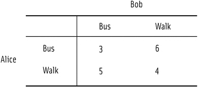
To calculate the Nash equilibrium, you must find the mixed strategies for each player that yield the best expected payoff when the other player is also choosing the best possible mixed strategy. In this example, Alice chooses Bus with probability p, and Walk with probability 1 – p (since the probabilities must add up to 1). Bob chooses Bus with probability q and Walk with probability 1 – q.
Alice can calculate her “expected payoff” for choosing Bus or Walk as follows. Her expected payoff from Bus will be the sum of:
Her payoff from Bus when Bob plays Bus, multiplied by the probability that Bob will play Bus, or 3 times q
plus
Her payoff from Bus when Bob plays Walk times the probability that Bob plays Walk, or 6 times (1 – q)
Her expected payoff from Walk is the sum of:
Her payoff from Walk when Bob plays Bus times the probability that Bob plays Bus, or 5 times q
plus
Her payoff from Walk when Bob plays Walk times the probability that Bob plays Walk, or 4 times (1 – q)
Summarizing,
Alice’s expected payoff for Bus = 3q + 6(1 – q)
Alice’s expected payoff for Walk = 5q +4(1 – q)
Applying similar reasoning to calculating Bob’s expected payoffs yields:
Bob expected payoff for Bus = –3p + –5(1 – p)
Bob expected payoff for Walk = –6p + –4(1 – p)
Now, Alice’s total expected payoff for the game will be her probability of choosing Bus times her Bus expected payoff, plus her probability of choosing Walk times her Walk expected payoff. Similarly for Bob. To achieve a Nash equilibrium, their probabilities for the two choices must be such that neither would gain any advantage by changing those probabilities. In other words, the expected payoff for each choice (Bus or Walk) must be equal. (If the expected payoff was greater for one than the other, then it would be better to play that choice more often, that is, increasing the probability of playing it.)
For Bob, his strategy should not change if
Applying some elementary algebra skills, that equation can be recast as:
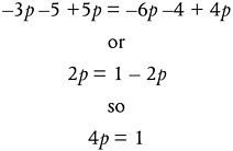
Which, solving for p, shows that Alice’s optimal probability for playing Bus is
So Alice should choose Bus one time out of 4, and Walk 3 times out of 4.
Now, Alice will not want to change strategies when
Which, solving for q, gives Bob’s optimal probability for choosing Bus:

So Bob should choose Bus half the time and Walk half the time.
Now let’s say Alice and Bob decide to play the hawk-dove game, in which the payoff structure is a little more complicated because what one player wins does not necessarily equal what the other player loses. In this game matrix, the first number in the box gives Alice’s payoff; the second number gives Bob’s payoff.
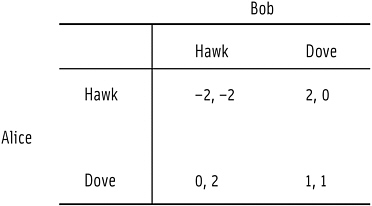
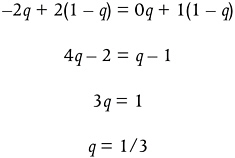
Alice plays hawk with probability p and dove with probability 1 – p; Bob plays hawk with probability q and dove with probability 1 – q. Alice’s expected payoff from playing hawk is –2q + 2(1 – q). Her expected payoff from dove is 0q + 1(1 – q). Bob’s expected payoff from hawk is –2p + 2(1 – p); his expected payoff from dove is 0p + 1(1 – p).
Bob will not want to change strategies when
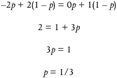
So p, Alice’s probability of playing hawk, is 1/3.