AI Applications for Automatic Pavement Condition Evaluation (2024)
Chapter: 2 Literature Review
CHAPTER 2
Literature Review
Road networks are important assets that need to be maintained at a reasonable degree of service through routine maintenance and rehabilitation treatments to address the progression of deterioration over time. Widespread use of pavement management systems, combined with pavement condition surveys, allow agencies to assess the current road network surface condition, project short- and long-term pavement performance, identify appropriate maintenance and rehabilitation treatments and timing, and determine budgetary needs. Current pavement condition assessment practices have transitioned from manual to APCSs using a variety of technologies. Advances in computing, data collection, and image processing and detection technology have made it possible to collect and analyze pavement surface conditions more easily than in the past.
McGhee (2004) and Pierce and Weitzel (2019) documented DOTs’ use of APCS techniques. In terms of evaluating pavement conditions, AI technologies continue to evolve and have proven to be a valuable tool in research and practical applications (Xu and Zhang 2022). AI can use data from a variety of sources, including pictures, videos, and sensors, to assess pavement surface condition. Typically, APCSs involve the use of 3D laser-based pavement imaging systems. More recent developments include analyzing 2D images from digital cameras or smartphones and processing with models based on ML/DL. AI technologies have a high degree of accuracy and efficiency in the detection and classification of pavement surface distresses, including cracking, rutting, and potholing (Sholevar et al. 2022). Pavement condition surveys that use AI technology can offer unbiased and reliable assessment, minimizing the subjectivity and data collection variability usually associated with manual pavement condition surveys. This chapter summarizes current APCS protocols and using AI to evaluate APCSs.
Historically, pavement conditions have been assessed using two primary methods: manual (e.g., walking or windshield) or semi- or fully automated surveys. In a walking survey, cracking and other distresses are measured by a certified rater based on the DOT’s distress protocols. Walking survey methods are time-consuming but can serve as a ground truth due to the precision of the data being collected. Windshield surveys are performed while driving at slow speed, with the certified rater estimating the extent and severity of distress. Windshield surveys provide less precision than walking surveys but can cover larger networks in less time. Semi- and fully automated pavement condition surveys can utilize similar data collection equipment; however, semiautomated methods include the use of a certified rater visually observing and noting the presence of distress (i.e., type, severity, and extent), while fully automated methods rely on software (e.g., AI) to identify distress (i.e., type, severity, and extent).
Automated Cracking Protocols
Several cracking and distress data collection protocols exist. The most relevant include:
- AASHTO R 86 (AASHTO 2022), Standard Practice for Collecting Images of Pavement Surface for Distress Detection;
- AASHTO R 85 (AASHTO 2018), Standard Practice for Quantifying Cracks in Asphalt Pavement Surfaces from Collected Pavement Images Utilizing Automated Methods;
- ASTM D6433 (ASTM 2023), Standard Practice for Roads and Parking Lots Pavement Condition Index Surveys;
- Distress Identification Manual for the Long-Term Pavement Performance Program (LTPP Distress Manual) (Miller and Bellinger 2014); and
- Surface Condition Assessment for the National Network of Roads (SCANNER) [United Kingdom (UK) Department for Transport 2021].
It is important to note that AASHTO R 85 (AASHTO 2018) and SCANNER protocols are inconsistent with ASTM D6433 (ASTM 2023) and the LTPP Distress Manual regarding cracking definitions, categories, and severity. The difference lies in the way the automated and manual surveys classify the cracking. AASHTO R 85 (AASHTO 2018) and SCANNER cracking protocols specify fewer cracking categories, while ASTM D6433 (ASTM 2023) and the LTPP Distress Manual were developed based on a walking survey to collect more cracking types for different types of surfaces. The following section provides a brief discussion of each protocol (Wang et al. 2020).
AASHTO R 86
AASHTO R 86 (AASHTO 2022) describes automated methods used to collect images to determine the presence of pavement surface distress. The standard does not specify the type of equipment but rather the following minimum criteria to ensure consistent data collection:
- The agency determines the lane and direction of travel for image collection.
- Images are at least 13 ft wide and no longer than 325 ft. Preferably, the image is 14 ft wide to include at least 12 in. of the shoulder to capture distress at the pavement edge.
- The image quality is capable of identifying:
- 33% of all cracks with a width less than 0.12 in.,
- 60% of all cracks with a width greater than or equal to 0.12 in. and less than 0.2 in., and
- 85% of all cracks with a width greater than or equal to 0.2 in.
Assessment is based on 10 100-ft samples with at least five such cracks per sample. The crack width must be within 20% or 0.04 in., whichever is greater, of the actual crack width at a confidence level of 85%.
- Pavement sections with no distress have less than 10 ft of false cracking (e.g., cracking detected but not present) over a 540 ft2 area. Assessment is based on 10 100-ft samples.
- Images may be captured using visible or infrared video, dimensional map, or any combination of technologies capable of meeting the standard criteria.
- The agency should confirm that the equipment can meet the criteria and includes checking the location accuracy, system stability and environmental impacts, validation, and quality control and assurance.
AASHTO R 85
AASHTO R 85 (AASHTO 2018) describes automated methods used to measure asphalt pavement surface cracking at the network level. Cracking can be measured with any equipment meeting the definitions stated by the standard (Table 1).
Table 1. Cracking definitions per AASHTO R 85 (AASHTO 2018).
| Crack Type | Definition |
|---|---|
| Longitudinal | Crack at least 12 in. long and oriented ± 20° relative to the lane centerline |
| Pattern | Interconnected cracks or a group of cracks in each area |
| Transverse | Crack at least 12 in. long and oriented 70° to 110° relative to the lane centerline |
| Other | All cracks not characterized as longitudinal, transverse, and pattern cracks |
Sample units of 52.8 ft long or less are used for the analysis. The standard divides the lane into five cracking zones (Figure 1).
Cracking zones are used to identify the location of longitudinal and pattern cracks. The extent of pattern cracking is measured by adding the length in feet or by the area influenced by the pattern cracks, and the severity is the average width detected in the sample unit. For longitudinal cracking and other cracking, the extent is reported by the sum of all crack lengths, and the severity is the average crack width. The extent and severity for pattern, longitudinal, and other cracks are reported for each cracking zone. The extent of transverse cracks is the sum of length of all transverse cracks within the sample unit, and the severity is the average width of the cracks. Cracks located in Zones 2 and 4 are assumed to be load related. Non-distressed sections are defined as containing less than 10 ft of false negative cracking (e.g., cracking is present but not detected) over a pavement area of 540 ft2 with a minimum of 10 100-ft long samples. The minimum standard for accurate crack detection includes:
- At least 85% of the cracks 0.2 in. or wider are mapped,
- At least 33% of cracks less than 0.12 in. and 60% of cracks from 0.12 – 0.2 in. wide are mapped, and
- At least 85% of crack lengths are recorded.
AASHTO R 85 (AASHTO 2018) also recommends establishing a ground truth by identifying a set of pavement images containing different crack types, extents, and severities and comparing the results to a 100% manual survey of the same pavement sections. Usually, this comparison is presented in a tabular form and includes crack type, severity, and the percentage of matching values between the two methods. Successful ground truth testing is defined by a 95% or better correlation between the image and the manual survey results.

ASTM D6433
ASTM D6433 (ASTM 2023) describes measuring pavement distress and severity to determine the pavement condition index (PCI). PCI is a composite measure of pavement condition and ranges from zero (very poor) to 100 (excellent). The ASTM D6433 (ASTM 2023) method recommends subdividing the pavement into samples, typically 20 contiguous concrete slabs or 2,500 ft2 of asphalt pavement. The PCI calculation is based on the visual measurement of pavement distress type, severity, and extent for each inspection sample. Distress types and severity levels for asphalt- and concrete-surfaced pavements are summarized in Tables 2 and 3 (Note: The extent of all distress types is number of slabs).
Table 2. ASTM D6433 (ASTM 2023) distress types for asphalt-surfaced pavements.
| Distress Type | Low Severity | Medium Severity | High Severity |
|---|---|---|---|
| Alligator cracking (ft2) | Fine, parallel, hairline, no spalling | Formed pattern, may be lightly spalled | Well-defined pieces, spalled at edges |
| Bleeding (ft2) | Visible a few days of the year, non-sticky | Visible several weeks per year, sticky | Extensive, considerably sticky |
| Bumps and sags (ft) and corrugation (ft2) | Noticeable vibration, no speed reduction | Significant vibration, some speed reduction | Excessive vibration, must reduce speed |
| Depression (ft2) | > 0.5 – ≤ 1 in. depth | > 1 – ≤ 2 in. depth | > 2 in. depth |
| Edge cracking (ft) (see block cracking for severity level) | No raveling | Some breakup and raveling | Considerable breakup or raveling |
| Joint reflection cracking (ft) | No-seal ≤ 0.38 in. or any filled crack | No-seal 0.38 – ≤ 3 in., no-seal ≤ 3 in. with secondary cracks, or sealed with secondary cracks | Medium or high severity with secondary cracks, no-seal > 3 in., or any with ~4 in. distress |
| Lane/shoulder drop (ft) | > 1 – ≤ 2in. | > 2 – ≤ 4in. | > 4 in. |
| Block (ft2), and longitudinal and transverse cracking (ft) | No-seal < 0.38 in. or any filled crack | No-seal > 0.38 – ≤ 3 in., no-seal ≤ 3 in. or filled with light, random cracks | No-seal with medium or high severity random cracks, no-seal > 3 in., or any with ~ 4 in. severely broken area |
| Patching (ft2) | Good condition, low or better ride quality | Moderate distress, medium ride quality | Badly deteriorated or high severity ride quality |
| Polishing (ft2) | Measure extent of affected area | ||
| Potholes (count) | 0.5 – 1 in. deep and 4 – 18 in. wide or 1 – 2 in. deep and 4 – 8 in. wide. | 0.5 – 1 in. deep and 18 – 30 in. wide, 1 – 2 in. deep and 8 – 18 in. wide, or > 2 in. deep and 4 – 18 in. wide | 1 – 2 in. deep and 18 – 30 in. wide or > 2 in. deep and 18 – 30 in. wide |
| Railroad crossing (ft2) | Noticeable vibration, no speed reduction | Significant vibration, some speed reduction | Excessive vibration, speed must be reduced |
| Raveling (ft2) | Not applicable | Aggregate loss > 20 per square yard | Very rough, pitted |
| Rut depth (ft2) | Mean > 0.25 – ≤ 0.5 in. | Mean > 0.5 – ≤ 1 in | Mean > 1 in. |
| Shoving (ft) | Noticeable vibration, no speed reduction | Significant vibration, some speed reduction | Excessive vibration, speed must be reduced |
| Slippage cracking (ft2) | Width ≤ 0.38 in. | > 0.38 width ≤ 1.5 in. | Width > 1.5 in. |
| Swell (ft2) | Noticeable vibration, no speed reduction | Significant vibration, some speed reduction | Excessive vibration, speed must be reduced |
| Weathering (ft2) | Loss of fines, fading asphalt color | Coarse aggregate exposure ≤ 0.25 in. | Coarse aggregate exposure > 0.25 in. |
Table 3. ASTM D6433 (ASTM 2023) distress types for concrete-surfaced pavements.
| Distress Type | Low Severity | Medium Severity | High Severity |
|---|---|---|---|
| Blowup | Noticeable vibration, no speed reduction | Significant vibration, some speed reduction | Excessive vibration, speed reduced |
| Corner break | ≤ 0.5 in., any sealed crack, no faulting | No-seal > 0.5 – ≤ 2in. or ≤ 2 in. and fault ≤ 0.38 in., or fault ≤ 0.38 in. | No-seal > 2 in., or any crack and fault > 0.38 in. |
| Divided slab | Low severity cracks with 4 – 8 pieces or medium severity cracks with 4 – 5 pieces | Low severity with > 8 pieces, medium severity with 6 – 8 pieces, or high severity with 4 – 5 pieces | Medium severity with > 8 pieces, or high severity with > 6 pieces |
| Durability “D” crack | ≤ 15% of slab | ≤ 15% of slab, most pieces loose or missing | > 15% of slab, most pieces missing |
| Faulting | > 0.13 – ≤ 0.38in. | > 0.38 – ≤ 0.75 in. | > 0.75 in. |
| Joint seal damage | Few locations of sealant debonding | Openings, pumping, or oxidized sealant | > 10% joint sealant debonded or missing |
| Lane/shoulder drop | > 1 – ≤ 2in. | > 2 – ≤ 4in. | > 4 in. |
| Linear crack | No-seal ≤ 0.5 in., any sealed crack with sealant in good condition | No-seal > 0.5 – ≤ 2 in., no-seal ≤ 2 in. and fault < 0.38 in., sealed and fault < 0.38 in. | No-seal > 2 in. or any fault > 0.38 in. |
| Patching | No distress | Moderately distressed | Badly distressed |
| Polished aggregate and pumping | Count number of affected slabs | ||
| Popouts | Measure > 1 per 3 ft2 | ||
| Punchout | Low severity with 2 – 5 pieces, or medium severity with 2 – 3 pieces | Low severity with > 5 pieces, medium severity with 4 – 5 pieces, or high severity with 2 – 3 pieces | Medium severity with > 5 pieces, or high severity with > 4 pieces |
| Railroad crossing | Noticeable vibration, no speed reduction | Significant vibration, some speed reduction | Excessive vibration, speed must be reduced |
| Scaling | Good condition, minor presence of scaling | Scaling ≤ 15% of slab | Scaling > 15% of slab |
| Shrinkage crack | Indicate presence only | ||
| Spalling, corner break | Depth ≤ 1 in. and > 5 x 5 in., or 1 – 2 in. and 5 x 5 – 12 x 12 in. | Depth > 1 – ≤ 2 in. and > 12 x 12 in., or > 2 in. and 5 x 5 – 12 x 12 in. | Depth > 2 in. and > 12 x 12 in. |
| Spalling, joint | Any tight pieces, loose pieces < 4 in. wide and < 1.5 ft long, or missing pieces < 4 in. wide and < 1.5 ft long | Loose pieces any width and > 1.5 ft long or missing pieces < 4 in. wide and > 1.5 ft long or > 4 in. and < 1.5 ft long | Missing pieces > 4 in. wide and > 1.5 ft long |
The accuracy of the pavement survey is based on identifying the pavement distress type (within 95%) and measuring linear distress (e.g., reflection cracking, edge cracking) within 10% and area (e.g., alligator cracking, polished aggregate) within 20%. PCI categories (e.g., good, fair, poor) are typically set by the agency and are dependent on the agency’s interpretation of acceptable levels of service.
The PCI calculation weighs the severity of each distress type as a function of impact on maintenance and rehabilitation requirements. For example, potholes have a higher PCI deduct value
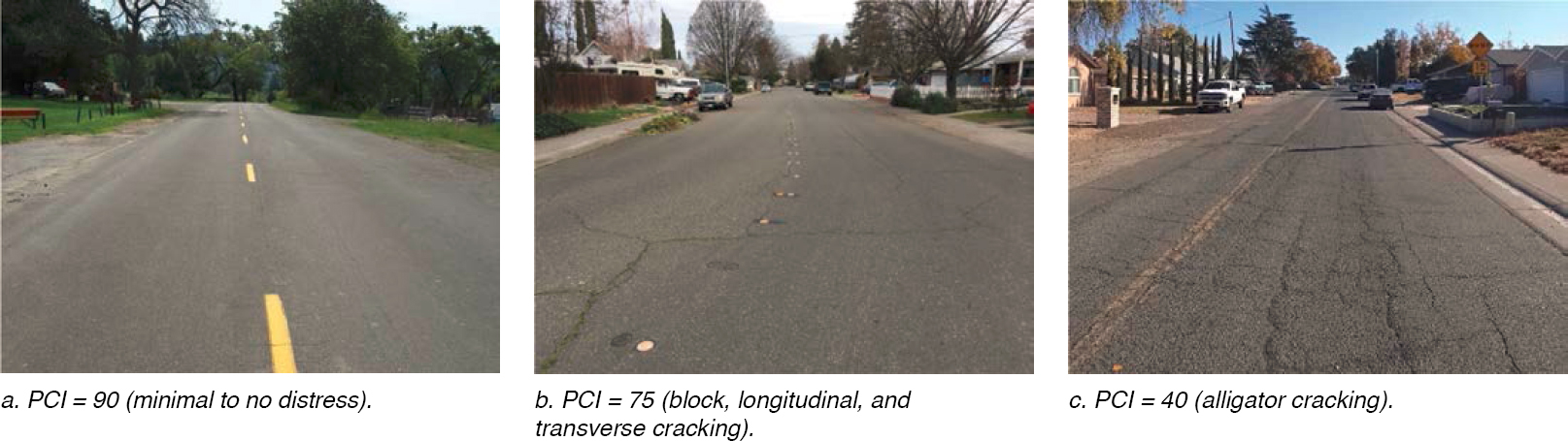
Figure 2. PCI category examples.
than alligator cracking, which has a higher deduct value than edge cracking. Examples of overall pavement condition are shown in Figure 2, and an example of PCI definitions is provided in Table 4.
LTPP Distress Manual
The LTPP Distress Manual was originally developed in 1987 (and revised over the following decades) to provide a consistent and uniform methodology for identifying and quantifying pavement distress. The LTPP Distress Manual follows similar principles as ASTM D6433 (ASTM 2023); however, a composite measure is not determined, and pavement distress is quantified according to pavement type instead (e.g., asphalt, jointed portland cement concrete, and continuously reinforced concrete), distress type, severity, and extent (Tables 5–7).
SCANNER
The SCANNER survey was first offered as a traffic-speed pavement condition survey for the main road network in the UK. In 2003 and 2004, the SCANNER method was adopted by local transportation authorities to determine pavement performance on “A” class roads in England. Today, the SCANNER survey is mandatory and used for all road classifications in England (UK Department for Transport 2021).
Table 4. Example of PCI score definition [U.S. Department of the Air Force (USAF) 2004].
| PCI | Category | Description |
|---|---|---|
| 100 – 86 | Good | Minor or no distress, routine maintenance recommended |
| 85 – 71 | Satisfactory | Low severity distress, routine maintenance recommended |
| 70 – 56 | Fair | Low and medium severity distress, routine to major maintenance recommended |
| 55 – 41 | Poor | Low to high severity distress, routine maintenance to reconstruction recommended depending on functional or structural distress types |
| 40 – 26 | Very poor | Mostly medium and high severity distress, challenges with applying maintenance treatments, needing more extensive repair |
| 25 – 11 | Serious | Mostly high severity distress, causing functional operation problems, needing immediate repair |
| 10 – 0 | Failed | Safe operation of vehicles no longer possible, requires reconstruction |
Table 5. LTPP distress types for asphalt-surfaced pavement (Miller and Bellinger 2014).
| Distress Type | Low Severity | Medium Severity | High Severity |
|---|---|---|---|
| Bleeding (ft2), raveling (ft2), and polishing (ft2) | Measure extent of affected area | ||
| Block (ft2), joint reflection (ft), longitudinal (ft) and transverse cracking (ft) | ≤ 0.25 in. wide or sealed crack, sealant in good condition | > 0.25 – ≤ 0.75 in. wide or any crack ≤ 0.75 in. with low random cracks | > 0.75 in. wide or any crack ≤ 0.75 in. with moderate to high random cracks |
| Edge crack (ft) | No breakup or material loss | Some breakup and material loss < 10% of length | Considerable breakup and material loss > 10% of length |
| Fatigue crack (ft2) | Few connecting cracks, no spalling or pumping, non-sealed | Interconnected, some spalling, no pumping, may be sealed | Complete pattern, spalled, may be sealed and pumping |
| Rut depth (in.) and lane/shoulder drop (in.) | Direct measure preferred | ||
| Patching (ft2) | Low severity distress, no pumping, rut ≤ 0.25 in. | Moderate severity distress, no pumping, rut > 0.25 – ≤ 0.5 in. | High severity distress, rut > 0.5 in., pumping or patching |
| Potholes (ft2) | ≤ 1 in. deep | > 1 – ≤ 2 in. deep | > 2 in. deep |
Similar to systems in the United States, the SCANNER survey uses laser-based equipment to measure the shape and texture of the pavement. Downward-facing digital cameras are mounted on a vehicle to collect images (typically 10.5-ft width) to quantify cracking, and a forward-facing video camera captures the driver’s perspective. The vehicles used for the data collection are certified on an annual basis, and the surveys are conducted by independent contractors (UK Department for Transport 2021).
Table 6. LTPP distress types for jointed concrete pavement (Miller and Bellinger 2014).
| Distress Type | Low Severity | Medium Severity | High Severity |
|---|---|---|---|
| Corner break (count) | Spall ≤ 10% length, no faulting, material loss, or patching, and broken ≤ 2 pieces | Low severity spall > 10% length, or fault ≤ 0.5 in., and broken ≤ 2 pieces | Spall moderate to high > 10% length, fault > 0.5 in., or broken > 2 pieces |
| Durability “D” crack (ft2) | Tight, no loose or missing pieces, no patching | Well-defined pattern, some small loose or missing pieces | Developed pattern, significant loose or missing pieces |
| Lane/shoulder drop or separation, faulting (in.) | Direct measure preferred | ||
| Longitudinal crack (ft) and transverse crack (ft) | < 0.12 in. wide, no spalling, faulting or sealed | ≥ 0.12 – < 0.25 in. wide, spalled < 3 in., or fault ≤ 0.5 in. | ≥ 0.5 in. wide, or spalled ≥ 3 in., or fault ≥ 0.5 in. |
| Longitudinal joint seal damage (ft) | Number of sealed joints and length of sealed joints with joint seal damage | ||
| Map crack/scaling (ft2) | Number of occurrences and square feet of affected area | ||
| Patching (ft2) | Low severity distress, no material loss or pumping, no faulting | Moderate severity distress, fault < 0.12 in., no pumping | High severity distress, fault ≥ 0.12 in., patched, pumping |
| Polishing (ft2) | Indicate potential reduction in surface friction | ||
| Spalling (ft) | ≤ 3 in. wide, no patching, or spalls | > 3 – ≤ 6 in. wide, loss of material | > 6 in. wide, spalled > 2 pieces, or patched |
| Transverse joint seal damage (count) | ≤ 10% of joint | > 10 – ≤ 50% of joint | > 50% of joint |
Table 7. LTPP distress types for continuously reinforced concrete pavement (Miller and Bellinger 2014).
| Distress Type | Low Severity | Medium Severity | High Severity |
|---|---|---|---|
| Blowups (count) | Count number of occurrences | ||
| Durability crack (ft2) | Tight, no loose or missing pieces, no patching | Well-defined pattern, some small loose or missing pieces | Developed pattern, significant loose or missing pieces |
| Lane/shoulder drop or separation (in.) | Direct measure preferred | ||
| Longitudinal crack (ft) | < 0.12 in. wide, no spalling, faulting or sealed | ≥ 0.12 – < 0.25 in. wide, spalled < 3 in., or fault ≤ 0.5 in. | ≥ 0.5 in. wide, or spalled ≥ 3 in., or fault ≥ 0.5 in. |
| Longitudinal joint seal damage (ft) | Not applicable | ||
| Map crack/scaling (ft2) | Not applicable | ||
| Patching (ft2) | Low severity distress, no material loss or pumping, no faulting | Moderate severity distress, fault < 0.12 in., no pumping | High severity distress, fault ≥ 0.12 in., patched, may have pumping |
| Polishing (ft2) | Not applicable, indicate potential reduction in surface friction | ||
| Punchouts (count) | Crack spalling < 3 in. or fault < 0.12 in., no material loss or patching | Crack spalling ≥ 3 – < 6 in., or fault ≥ 0.12 – < 0.25 in. | Crack spalling ≥ 6 in. or punched down ≥ 0.25 in., or loose, or broken > 2 pieces |
| Spalling (ft) | < 3 in., no material loss or patching | ≥ 3 – < 6 in., material loss | ≥ 6 in., material loss, broken > 2 pieces, or patched |
| Transverse crack (ft) | Spalling ≤ 10% of length | Spalling > 10 – ≤ 50% of length | Spalling > 50% of length |
| Transverse joint deterioration (count) | No spalling or fault ± 2 ft of joint | Spalling < 3 in. within ± 2 ft of joint | Spalling ≥ 3 in. within ± 2 ft of joint |
The SCANNER survey collects the longitudinal profile, transverse profile, edge condition, and texture of the road and the presence and extent of cracking (Table 8).
Cracking is quantified using a crack map and includes crack length, offset position, angle, and type (i.e., joint or crack). Total cracking is estimated by overlaying a crack map with a grid and adding the areas of the grid squares containing cracks. Each pavement cell is 8 in. by 8 in., and the size of the grid map is 20 cells long (approximately 13 ft) and 16 cells (approximately 11 ft) wide (Figure 3) (UK Department for Transport 2021).
Transverse cracking is defined as a crack covering an area of at least two cells in the longitudinal direction and the entire width of the lane (Figure 4). In Figure 4, 13 cells within a 1.3 ft length in the longitudinal direction and across the full survey width were identified to contain a crack. Within the sample area, 32 cells, or 41%, contain a crack. Since more than 20% of the total cells within this area have been identified as containing a crack, the cells are defined as a transverse crack.
The intensity of wheel path cracking is measured by first examining the position of the crack to determine whether it falls within the wheel path area. The wheel path area is defined as an area approximately 2 ft to both the right and left of the survey centerline with a wheel path width of 2.6 ft (Figure 5). A wheel path crack occurs when 80% of the detected crack is within the wheel path area (UK Department for Transport 2021).
Table 8. SCANNER data collection.
| Distress or Condition Type | Definition |
|---|---|
| Rut depth (in.) | Based on transverse profile measurements, averaged over 4 in. intervals. |
| Longitudinal profile | Based on longitudinal profile measurements. |
| Texture (in.) | Macrotexture measured at 0.04 in. intervals and averaged over 33 ft. |
| Cracking | Processing downward-facing images using automatic crack detection software, describes transverse and longitudinal location, length, and angle (relative to direction of traffic) of the crack. |
| Edge deterioration | Measured from transverse profile at pavement edge, reported on 33 ft intervals. |


AI and ML/DL
AI can be defined as a series of robust computational algorithms and statistical models capable of adapting and learning from data patterns. AI technology has been increasingly incorporated into pavement engineering research and practice and related fields because of the continuous advancement in automatic data acquisition devices, computer vision techniques, and ML/DL algorithms (Majidifard et al. 2020a, Hou et al. 2021, Guerrieri and Parla 2022, Sholevar et al. 2022, Xu and Zhang 2022).
AI is used with pavement condition surveys to automatically identify and classify different types of distresses. The use of AI has notable advantages, including data collection automation, accurate models when trained using large databases, and real-time monitoring. A significant challenge in using AI for pavement condition assessment is data availability (i.e., getting a representative and sufficient number of data set images that have been labeled with pavement distresses). The AI models also need to be trained using a wide range of pavement distresses (type and severity) to accurately classify the proper condition. Lastly, it is important to understand the AI model architecture to interpret and trust the results.
AI models and techniques will be discussed in the following sections; however, a brief description of the process for pavement distress detection is as follows:
- Collect a representative data set of images from a road network,
- Label the images with the proper distress types and severities,
- Conduct pre-image processing to remove any noise in the images,
- Build an AI model for image analysis that can extract the features of the labeled images (i.e., an AI model will learn those features corresponding to pavement distresses), and
- Apply the AI model to the data set (typically, 70%) for training purposes, and use the remainder of the data set (typically, 30%) for model validation.
Data Acquisition
Digital image processing technologies have been applied widely to pavement condition assessment. For example, digital cameras have been used to detect cracks, and laser scanning has been used to determine rut depth and the International Roughness Index (IRI). Image technologies have also been employed for jointed plain concrete pavement, joint faulting, pavement texture, and pothole identification. More recently, cameras and light detecting and ranging (LiDAR) systems in unmanned aerial vehicles have been used to identify pavement distresses and roughness (Du et al. 2021). Figure 6 illustrates currently used data acquisition methods, each of which are described briefly in the following sections.
Vision-Based
Extensive effort has been dedicated to processing images from digital cameras mounted to vehicles to detect cracking, permanent deformation, and surface texture (Du et al. 2021). Conventional image processing and traditional ML/DL models are typically used to perform image analyses (Sholevar et al. 2022). Figure 7 illustrates the use of digital images to identify surface distress from a dashboard-mounted smartphone.
3D Imaging
Laser-based technologies, line projection, and ground penetrating radar are technologies employed to capture 3D images. 3D laser scanning data has become the predominant approach for automatic pavement condition data collection due to its ability to gather depth information and its robustness to lighting conditions relative to that of 2D images (Wang et al. 2017; Zhang et al. 2018). Most 3D data acquisition systems use triangulation (i.e., laser line profiling) and

structured illumination (i.e., patterns of light used to define an object’s geometric shape and depth), projecting a laser line onto the object being measured. A digital area scanning camera is placed at a defined distance and angle from the light source. The camera is equipped with either a charge-coupled device (CCD) or a complementary metal-oxide semiconductor (CMOS) sensor. The camera captures pictures in structured illumination, and the image is analyzed by examining the deformations of the laser lines on the object. This examination allows the depth (z-axis) and the horizontal position (x-axis) of each point to be determined (Figure 8). To obtain the y-axis position, the 3D system is typically paired with an encoder (Tsai and Li 2012).
Vibration-Based
Inertial profiler systems include an accelerometer to measure the vertical vibration of the vehicle, sensors to measure the relative movement between the road surface and the vehicle, and a distance-measuring instrument to record the distance traveled along the roadway (Figure 9).
Most recent research has used DL/ML to analyze vibration measurements from accelerometers to quantify pavement roughness (Liu et al. 2019; Aboah and Adu-Gyamfi 2020). The vibrations collected by static accelerometers or smartphones can be used to measure roughness and to detect other distresses, such as potholes (Eriksson et al. 2008; Medina et al. 2020). Other researchers

Figure 7. Surface distress detection using a dashboard-mounted smartphone.

have investigated the use of vibration sensors installed in the pavement and use ML techniques to detect pavement deterioration (Takanashi et al. 2020; Gao et al. 2021).
Most smartphones have cameras that can capture high resolution images from pavements to detect pavement distresses, such as cracking and potholes (Huyan et al. 2020; Chitale et al. 2020). They also have embedded sensors, such as accelerometers and GPS sensors. In the past decade, accelerometers embedded in smartphones have gained popularity as an alternative low-cost tool to measure car vibrations (Islam et al. 2014; Bridgelall 2015; Bridgelall and Tolliver 2018; Medina et al. 2020). Figure 10 shows a smartphone collecting vibration data.
AI Models
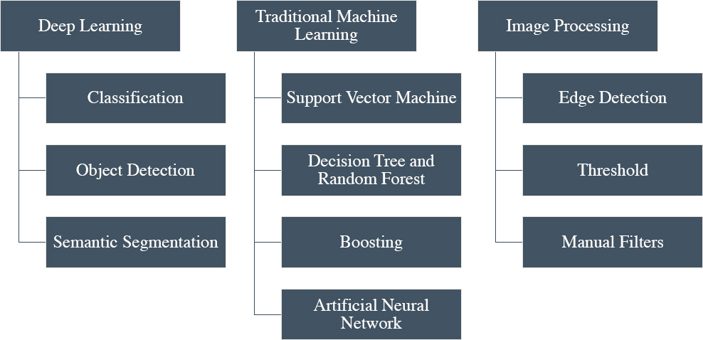
ML/DL techniques have shown to be successful for many types of problems involving computer vision applications (Guerrieri and Parla 2022), including identifying pavement distresses and other civil engineering applications. Figure 11 illustrates the image analysis methods used to detect pavement distresses (Sholevar et al. 2022). The following sections provide a brief description of each image analysis method.

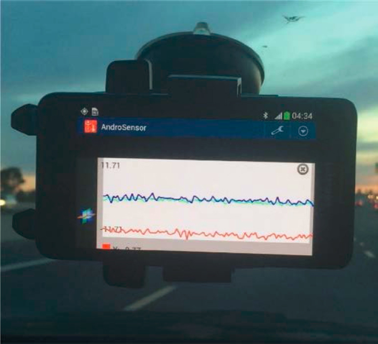
Figure 10. Example of a smartphone collecting vibration data.
DL
In civil engineering and intelligent transportation systems, DL approaches have emerged as the most frequently used computational strategy, producing comparable results between pavement condition surveys and field conditions (Zhu et al. 2021; Ranyal et al. 2022). The capacity of DL to learn large amounts of data is one of its advantages. Another advantage, particularly over conventional ML or other image processing methods, is that the data-driven, end-to-end learning process is more accurate, more accessible, and faster (Sholevar et al. 2022). Deep convolutional neural networks (CNNs) have assumed the utmost relevance in performing vision-based tasks as a result of the quick development of DL approaches. Classification, object detection, and picture segmentation are the main pattern recognition tasks carried out by vision-based DL algorithms (Ranyal et al. 2022).
Classification
Classification methodology divides an image into blocks and assigns each block a target class by using the sliding window technique to analyze images of any size. CNNs with a simple design are used in image classification models to extract features or patterns from pictures (Sholevar et al. 2022). The classification detection method is helpful when making decisions about whether a picture contains the desired object, an anomaly, or nothing. Localization, which establishes the location of the identified object, is a notable classification function (Ranyal et al. 2022). Figure 12 illustrates an example of DL classification and how the image is broken down into smaller blocks to classify the crack.
Object Detection
Object detection methodology combines classification and localization to identify the items in an image and determine their locations. Bounding boxes are used to demonstrate the detection and position of an object when applying categorization to different objects (Ranyal et al. 2022). Object detection architectures like You Only Look Once (YOLO), Regions with CNN, and Single-Shot Detector (SSD) are widely used for pavement distress detection because of their speed, simplicity, and capacity to search within a large image for any number of predefined distresses. These benefits make object detection the most practical method for identifying the location and severity of pavement distresses in large, complicated images (Sholevar et al. 2022). Figure 13 shows an example of road damage detection using object detection. As seen in the figure, the model detects longitudinal cracking (blue box); however, even in trained data sets, it is difficult to differentiate between cracks and shadows usually caused by light posts or overhead power lines (red box).
Semantic Segmentation
By dividing an image into sections, semantic segmentation extracts potentially significant portions of the image for further processing using classification and object detection depending on its shape and borders. By highlighting the foreground features, semantic segmentation makes

Figure 12. Example of DL classification.

Figure 13. Example of object detection.
it easier to assess the objects. Semantic segmentation, as opposed to classification and object detection, shows pixel by pixel features of an item, as seen in Figure 14 (Ranyal et al. 2022). Fully convolutional networks and encoder-decoders are the two most common architectures for segmentation models (Sholevar et al. 2022).
A summary of advantages and limitations of the DL method is summarized in Table 9.
Table 10 provides a list of studies that have used DL in pavement distress detection.

Figure 14. Example of crack segmentation and pixel by pixel feature extraction.
Table 9. DL Method advantages and limitations (Ranyal et al. 2022; Sholevar et al. 2022).
| Method | Advantages | Limitations | Accuracy |
|---|---|---|---|
| Classification |
|
| 90-97% |
| Object Detection |
|
| 70-99% |
| Semantic Segmentation |
|
| 70-97% |
Table 10. DL research studies (Sholevar et al. 2022).
| Reference | Distress Types Identified | ||||||
|---|---|---|---|---|---|---|---|
| None | Bumps | Bleeding | Cracking | Patching | Potholes | Rutting | |
| Nguyen et al. 2018 | √ | ||||||
| Shah and Deshmukh 2019 | √ | √ | √ | ||||
| Eisenbach et al. 2017 | √ | √ | √ | √ | |||
| Fan et al. 2019 | √ | ||||||
| Nie and Wang 2018 | √1 | √ | |||||
| Lei et al. 2020 | √1 | √2 | √ | √ | |||
| Commandre et al. 2017 | √3,4 | ||||||
| Anand et al. 2018 | √ | ||||||
| Maeda et al. 2018 | √ | √ | √ | √ | |||
| Song et al. 2020 | √ | ||||||
| Zhang et al. 2017 | √ | ||||||
| Chen et al. 2020 | √ | ||||||
| Konig et al. 2019 | √ | ||||||
| Yang et al. 2020 | √ | ||||||
1 deformation.
2 included crack sealing
3 study also identified utility covers
4 fatigue and transverse cracking
Note: √ indicates distress type identified in the research study
Traditional ML
Traditional ML models analyze patterns to classify and quantify pavement condition information. Typical ML technologies include (a) support vector machine (SVM) method, (b) decision tree (DT) and RF, and (c) bootstrap aggregation.
SVM Method
The SVM method is frequently used for solving regression and classification problems. The SVM method depends on extracting high-quality features from the image (Cao et al. 2020). The model features (e.g., pavement distress) must be very well defined to ensure model reliability. In addition to pavement distress detection, SVM methods have been used for cancer detection, financial forecasting, picture classification, digital handwriting recognition, and facial expression classification (Hoang et al. 2018; Xu and Zhang 2022). SVM methods use a hyperplane in the input variable space to split the positive and negative training samples. Typically for pavement crack detection, the image is preprocessed or filtered to a smooth texture to enhance the existing defect or cracks. The image is subdivided into blocks, with each block producing a feature or support vector. Finally, the SVM method is used to detect and classify cracks, potholes, and other defects using the information in the support vector structure (Daniel and Preeja 2014).
DT and RF
DT algorithms are also commonly used for regression and classification. DTs have a hierarchical structure consisting of a root node (or first splitting node), branches to connect to internal nodes or decision/attribute nodes, and leaf nodes, which represent all possible outcomes within the data set. This process is applied to all data sets iteratively until all or most of the data points are classified. RFs are algorithms that combine the output from DTs to achieve a single result. DT and RF models have also been developed for pavement distress detection (Cubero-Fernandez et al. 2017; Hoang and Nguyen 2019). The output of each DT is evaluated to detect a feature classification (i.e., crack detection), with the majority or average results reported as the final output. Figure 15 shows an example of the RF crack definition process from the original image to the final output.
Bootstrap Aggregation
Bootstrap aggregation, or bagging, is an ML technique typically used in DT techniques to improve the stability and accuracy of the AI models. The bootstrap aggregation technique randomly creates multiple subsets to train a separate model, then combines (or aggregates) the predictions of each separate model into a final prediction model. Ahmad et al. (2023) developed an ML architecture using bootstrapping to improve the accuracy of pavement crack detection and segmentation from different data sets.
Boosting
Boosting refers to a generic and efficient approach combining imprecise and inaccurate classifiers to produce an accurate prediction rule. In other words, boosting is founded on the idea that discovering several imprecise rules of thumb or classifiers is sometimes far simpler than discovering a single, extremely precise prediction rule (Schapire 2003). To achieve the desired outcome, a training set of data is scanned repeatedly, letting the learning algorithm concentrate on the cases incorrectly identified in previously repeated scans (the “hardest cases”). Judgments made using a weighted mixture of the unreliable classifiers can provide results with higher accuracy than individual weak classifiers (Schapire and Freund 2013). Traditional crack detection models may contain a high number of false detections, and the Adaptive Boosting (AdaBoost) model is frequently used to improve model accuracy (Xu et al. 2022). AdaBoost model operation is examined in depth using a range of techniques by paying close attention to the risk of overfitting to the training set.
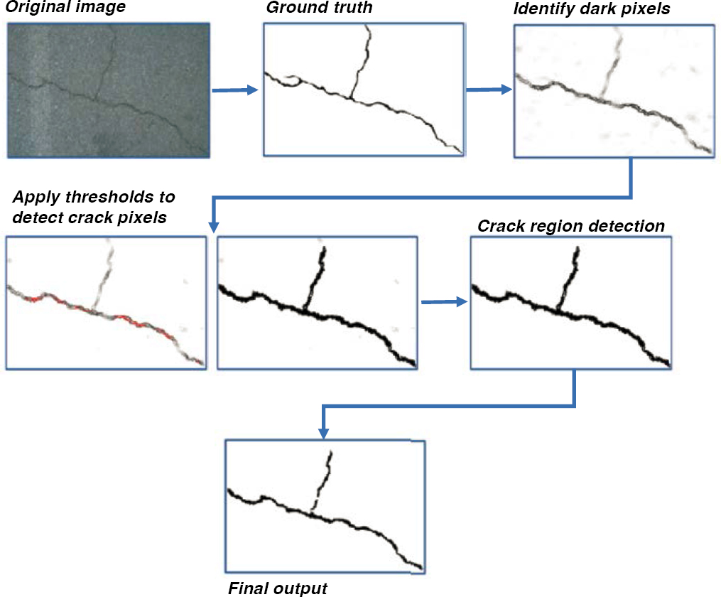
Figure 15. Example of RF crack definition.
The evaluation of “confidence” measures for the weak classifiers can improve the model and discrimination rules even after the training set is correctly categorized (Cord and Chambon 2012; Schapire and Freund 2013). Figure 16 compares the output for a boosting method to the original and ground truth images from different data sets. Ground truth images are manually processed to isolate desired features (e.g., cracks) from the original image and create a label with these features.
Artificial Neural Networks
Artificial neural networks (ANNs) are information processing architectures made up of several basic processing elements, or “neurons,” interconnected in a parallel manner. Each neuron has the ability to share its outputs, if any, to and accept weighted inputs from many other neurons. Throughout the weighted interconnections, information is represented in a distributed manner. A collection of patterns is repeatedly given to the ANN during a training session, and the ANN learns the class to which each of the input patterns belong. Figure 17 provides an example of crack detection used by an ANN model. Advantages and limitations of the traditional ML method are summarized in Table 11.
Table 12 provides a summary of relevant efforts for pavement distress detection using traditional ML models.
Image Processing
Traditional image processing refers to filtering noise captured by digital cameras or imaging sensors. In pavement condition assessment, images can be affected by shadows, rain, stains, and other factors. Usually, cracking in an image shows a thin, irregular shape along with dark lines bounded by noise. Typical image processing methods include the following items described in the subsequent section:
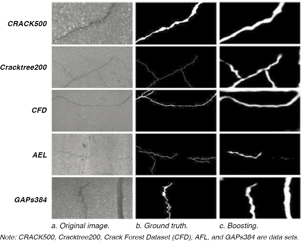
Figure 16. Example of boosting.
Edge Detection
Edge detection methods are able to clearly identify the crack outline. A differential function is used to determine edge information based on a crack’s grayscale change (Hou et al. 2021). Several edge detection methods exist (referred to as operators), including Sobel, Prewitt, Roberts, and Canny (Cao et al. 2020).
Thresholding
Thresholding-based methods have been widely used for crack detection since the 1980s due to their simplicity and effectiveness (Oliveira and Correia 2009, Li et al. 2015, Zhou et al. 2016, Cao et al. 2020). These methods determine whether a pixel belongs to the target area or whether the

Figure 17. Example of ANN model for crack definition.
Table 11. Advantages and limitations of traditional ML methods (Sholevar et al. 2022, Xu and Zhang 2022).
| Method | Advantages | Limitations | Accuracy |
|---|---|---|---|
| SVM |
|
| 78 – 98% |
| DT and RF |
|
| 80 – 98% |
| Boosting |
|
| 85 – 98% |
| ANNs |
|
| 92 – 98% |
background characteristic attributes meet the set threshold values. In this way, a gray image can be transformed into a binary image. The key to this method is identifying an acceptable threshold value.
Region Growing
Another method for detecting pavement cracks is the recognition technique, which is based on region growing. This method was proposed and adopted in the Texas Department of Transportation’s APCS in the mid-2000s. The region growing method can be used to identify the edge distribution of crack defects and draw the crack contour but cannot provide a description of the information contained within the crack’s internal pixels. Through the use of image characteristics
Table 12. Traditional ML research studies for pavement condition assessment.
| Reference | Cracking | Diagonal Cracking | Longitudinal Cracking | Potholes | Rutting | Transverse Cracking | |
|---|---|---|---|---|---|---|---|
| H. Li et al. 2019 | √ | ||||||
| Ai et al. 2018 | √ | ||||||
| B. Li et al. 2019 | √ | ||||||
| Ahmadi et al. 2021 | √ | √ | √ | √ | |||
| Cao et al. 2021 | √ | ||||||
| Pan et al. 2018 | √ | √ | |||||
| Oliveira and Correia 2013 | √ | ||||||
| Moussa and Hussain 2011 | √ | ||||||
| Lin and Liu 2010 | √ | ||||||
| Pan et al. 2017 | √ | √ |
Note: √ indicates distress type identified in the research study
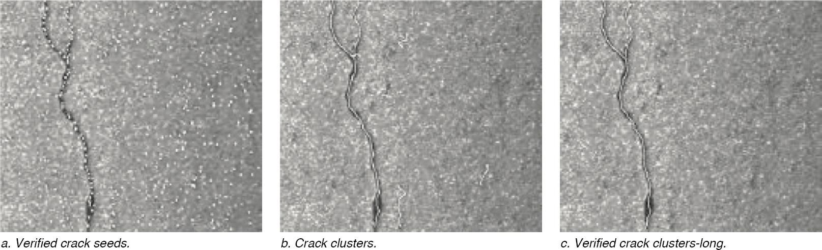
Figure 18. Example of recognition technique based on region growing method.
(e.g., border cell contrast and pixel brightness), the original image is transformed into a grid of cells (8 × 8 pixels), and each cell is categorized as either a crack (i.e., seed) or non-crack cell (Figure 18). Seed clusters are then formed from the crack seeds and crack features are extracted (Huang and Xu 2006; Zhou et al. 2016). Gathering similar pixels to form a region is the fundamental concept behind the region-growing algorithm. The accuracy of image segmentation is greatly affected by the seed selection (Cao et al. 2020).
Manual Filters
Manual filters are applied to isolate the desired features from an image. Typically, the image is converted into binary code before the threshold filters are applied. Figure 19 illustrates an example of manually isolating a crack from an image. Manual filters are time-consuming and, therefore, are not practical for network level APCSs.
Factors Affecting AI Models
It is important to consider the impact of data assumptions prior to using AI algorithms for pavement distress evaluation. The accessibility of the data used to train and test the AI algorithm has a substantial impact on its performance. Since data are the basis of all AI-oriented models,
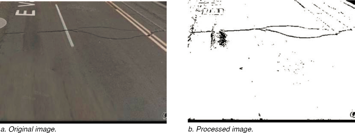
Figure 19. Example images of manual threshold segmentation.
the absence of valid data can seriously weaken the method’s validity. For example, if the data used for training any model fail to provide a ground truth, any results obtained from the model will not be valid (Xu et al. 2022). Furthermore, accurate pavement distress detection exponentially increases model accuracy with more training images (Ranyal et al. 2022). The factors affecting AI models include data quality and diversity, data preprocessing, model architecture and training, and overfitting.
Data Quality and Diversity
Data quality for model training has a significant impact on model robustness. Image quality can also significantly affect any proposed model, and the presence of image noise can affect the detection of pavement distress or the classification model (Majidifard et al. 2020b, Xu et al. 2022). It is important to gather a diverse and comprehensive data set of images covering various scenarios and variations (i.e., different types of distresses with different illumination). The data set should include labeled images to train the model effectively.
The image size required for AI mode training can vary depending on the specific task and the architecture of the model being used. However, some general considerations should be kept in mind:
- The image size should be compatible with the architecture of the AI model;
- The larger the image, the more computational effort will be required;
- The image size should be chosen based on the features to be extracted (e.g., minimum size required to detect cracking or other distresses); and
- Many of the data sets used to train AI models come from private sources, making it difficult to compare models. Approximately 78% of the AI distress models are trained on private data sets; only 22% are trained on public data sets.
Table 13 provides a description of the type of processing task, the device used for data collection, the number of images, and the image size for some of the open-source data sets.
Data Preprocessing
Data preprocessing refers to the action of modifying data before they are used to improve their performance. The input variables should be carefully chosen and optimized for the AI algorithm. Preprocessing the image and data set is a typical step in AI models for distress detection applications and may include removing unrelated features or objects, resizing the inputs, and augmenting the data to improve the initial data set and avoid model overfitting (Wang and Hu 2017, Ghasemi et al. 2018, Chun et al. 2021, Hsieh and Tsai 2021, Sholevar et al. 2022). Other preprocessing techniques include removing image noise, resizing, cropping, gray scaling, and normalization (Sholevar et al. 2022). In some cases, noise can be detected. In Figure 20, noise is very difficult to detect because the crack and noise patterns are very similar.
Model Architecture and Training
It is important to choose the correct AI architecture for the image processing task. For pavement distress detection, a model capable of extracting image features and spatial relationships is very important. For training purposes, AI models can be broadly classified into supervised, unsupervised, and reinforced learning (Praveena and Jaiganesh 2017). Supervised and unsupervised training are commonly used methods for crack and pavement distress analysis.
The goal of supervised training techniques is to identify the link between input (i.e., independent variable) and target attributes (i.e., dependent variable). A model serves as a representation of the identified relationship. Developed models describe and explain hidden events within a data set and may be used to predict an attribute’s target value, given the values or labels of its
Table 13. Public data sets (Arya et al. 2021, Ranyal et al. 2022, Sholevar et al. 2022, Xu et al. 2022, Zhu et al. 2022).
| Data set | Task Type | Device | Distress | No. of Images | Resolution |
|---|---|---|---|---|---|
| CDF | Segmentation | iPhone 5 | Cracking | 118 | 480x320 |
| Aigle-RN | Segmentation | Professional camera | Cracking | 38 | 991x462, 311x462 |
| Crack500 | Segmentation | LG-H345 | Cracking | 500 | 2000x1500 |
| German Asphalt Pavement Distress (GAPs v1) | Object detection | Professional camera | Several Distresses | 1,969 | 1920x1080 |
| GaMM | Segmentation | Professional camera | Cracking | 42 | 1920x480 |
| Cracktree200 | Segmentation | N/A | Cracking | 206 | 800x600 |
| CrackIT | Segmentation | Optical | Cracking | 84 | 1536x2048 |
| EdmCrack6001 | Segmentation | GoPro 7 | Cracking | 600 | 1920x1080 |
| GAPs v2 | Object detection | N/A | Cracking, pothole, patch, open joint | 2,468 | 1920x1080 |
| Pavement image data set | N/A | Google application | Several distresses | 7,237 | N/A |
| Street-view images | N/A | Smartphones | Several distresses | 9,053 | N/A |
| Road Damage Dataset | Object detection, classification | Smartphones | Several distresses | 26,336 | 600x600 and 720x720 |
| Deep Crack | Segmentation | N/A | Crack | 537 | 544x384 |
| Unmanned Asphalt Pavement Distress | Object detection | Unmanned aerial vehicles | Several distresses | 3,151 | 5632x3584 |
1EdmCrack600 is a data set from roads in Edmonton, Canada.
N/A= Not Available
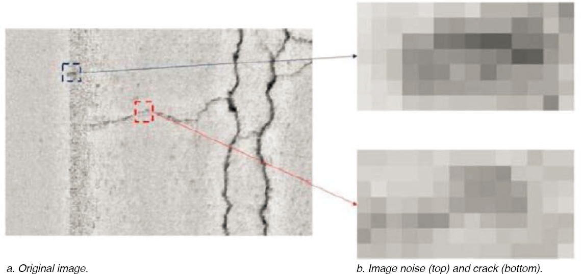
Figure 20. Example of image noise.
input attributes (Cao et al. 2020). Common supervised models include SVM, ANN, and RF (Chou et al. 1994, Li et al. 2009, Nguyen et al. 2009, Moussa and Hussain 2011, Del Rio-Barral et al. 2022).
Unsupervised training, also referred to as data mining, occurs when the data do not contain labels. This means data samples have no recognized output results, and the model needs to learn relationships between samples and then classify them. The advantage of using unsupervised training is the elimination of human influence and subjectivity in creating labels (Cao et al. 2020).
Unlike supervised and unsupervised learning, reinforced learning (RL) is a unique AI technology. While the goal of extrapolating or generalizing the information gained from a training set of labeled examples in supervised learning is to have the system to respond appropriately to new input and the goal of unsupervised learning is to determine the structure of the unlabeled data, the goal of RL is to maximize the overall cumulative reward. RL involves learning by trial and error based on the feedback acquired from the interaction between agents and the environment, as opposed to learning from examples of appropriate conduct (Xu et al. 2022).
Overfitting
In AI, overfitting refers to the algorithm behavior that occurs when the model accurately predicts the data from the trained data set but cannot accurately generalize to a new data set. Figure 21 shows an example of overfitting. The model was trained and validated using images from a different data set. When the model was used with new images, the model erroneously detects a moderate severity patch bound by a blue line and cracks/open joints bound by red lines.
A common technique to address overfitting is referred to as gradient boosting (GB). GB combines the predictions from many weak classifiers to create a single, strong classifier. By building a separate tree each time, GB can get around the primary flaw of DT models (overfitting) by calibrating mistakes introduced by earlier trees and adjusting the weights of the observations. Another way to minimize overfitting is to train a model with randomly selected images (70% of the data set) and use approximately 15% of the images for validation and the other 15% to evaluate the final AI model fit. Typically, the validation data set is used to calibrate or tune the AI model, providing an unbiased assessment; however, the increased use of the validation data set can result in a more biased AI model.

Figure 21. Example of overfitting.
Data Acceptance
Ground Truth
Ground truth is a commonly used term that refers to the correct or true value of a specific observation or problem. Cracks and other distresses are digitized manually using ground truth images or field measurements (Figure 22). The Hausdorff scoring method is commonly used to compare the AI models to the ground truth results. The Hausdorff method provides a score that ranges from 0 to 100, with 100 representing perfect distress segmentation (Oliveira and Correia 2009, Tsai et al. 2012, and Zhang et al. 2018).
Model Validation
Typical evaluation metrics for ML/DL models include precision, recall, and accuracy. Precision is the ratio of the correct detected results to all the detected results. Recall is the ratio of the correct detected results to all the ground truth results. The F1 score is commonly used to determine model accuracy and is the harmonic mean of precision and recall. The F1 score is typically preferred over other statistical metrics due to its ability to balance precision and recall. Table 14 summarizes typical model evaluation metrics.
Model validation of detected distresses is one of the primary tasks for evaluating ML/DL models. In addition to the performance metrics described above, other methods used to validate models include cross-validation, the holdout method, k-fold cross-validation, and leave-one-out cross-validation.
In ML, cross-validation refers to the process in which models are trained on subsets of the input data and then evaluated on the complementary subset data. The purpose of cross-validation is to detect data overfitting, identify any bias, and provide an understanding of whether the model will generalize with other independent data sets. The difference between cross-validation and k-fold cross-validation is the k-value refers to the number of groups that will be used to train and test the ML/DL models. The holdout method differs from the cross-validation method in the way the training and testing data are split. In the holdout method, the data set is split into the training and testing set only once; in the cross-validation process, the data set is split randomly and in multiple folds or data sets. The leave-one-out cross-validation method is typically used when the data set is small or when the precision is more important than the computational cost since this method includes more training-test iterations than other methods. This method considers each observation as the validation set and the rest of the observations as the training data set. The process repeats the validation process for each observation, resulting in a large computational cost.
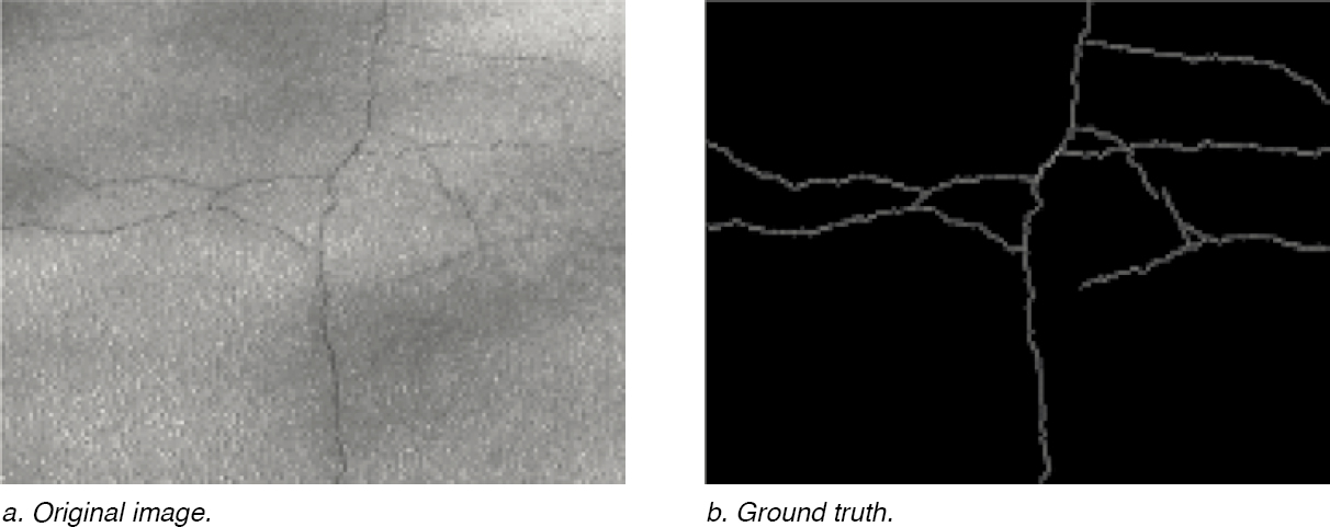
Figure 22. Example of manually setting ground truth.
Table 14. AI model performance measures (Eisenbach et al. 2017).
| Measure | Definition1 |
|---|---|
| True positive rate | |
| True negative rate | |
| Precision | |
| Balanced error rate | |
| Accuracy | |
| Matthews correlation coefficient | |
| G-mean | |
| Area under the Receiver Operator Characteristic (ROC) curve | |
| F1 score | |
| G-measure | |
| Break-even point | |
| Area under the precision recall curve |
1tp = number of true positives, fn = number of false negatives, fp = number of false positives, and tn = number of true negatives.
Summary
This section provided a literature review of the current automated pavement condition assessment protocols, such as AASHTO R 85 (AASHTO 2018), ASTM D6433 (ASTM 2023), LTPP Distress Manual, and SCANNER. It also included an overview on the use of AI technology for APCS. APCS analysis using AI methods includes:
- Data acquisition using vision-based (e.g., digital cameras), 3D imaging, or vibration-based (e.g., accelerometers) systems;
- Modeling using DL (e.g., classification, object detection, and semantic segmentation), ML (e.g., SVM, decision tree, RF, boosting, and ANN), and image processing e.g., (edge detection, threshold, and manual filters) methods; and
- Data acceptance based on ground truth testing (e.g., manual versus AI results, image review versus AI results) and model validation based on precision, recall, and the F1 score.
The literature review also identified several factors affecting AI models. These factors included data quality and diversity (e.g., image quality, image noise, different distress, different illumination levels), data preprocessing (e.g., removing features, resizing images, and data augmentation), model architecture and training (e.g., capable of extracting image features, spatial relationships), and overfitting (e.g., model accurately predicts from the trained data set but inaccurately on a new data set).


