Observing and Modeling Wildland Fires and Their Greenhouse Gas Emissions: Opportunities and Challenges

The second day of the workshop focused on the tools used to quantify greenhouse gas (GHG) emissions from wildland fires and better understand the impact of fires on the net carbon budget. The first session focused on observational-based approaches for quantifying emissions and the second session focused on modeling approaches. Both sessions as well as the breakout discussions on the second day sought to identify key challenges and gaps that could improve understanding of GHG emissions from wildland fires today and in the future and inform potential mitigation strategies.

OBSERVATION-BASED APPROACHES FOR QUANTIFYING EMISSIONS FROM WILDLAND FIRES

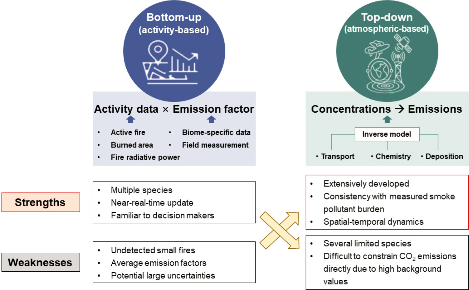
Bo Zheng, Tsinghua University, described the importance of accurately quantifying emissions from wildland fires to inform mitigation and adaptation policies. Broadly, there are two methods to estimate GHG emissions from fires: (1) activity-based (or “bottom-up”) approaches combine activity data about fires with emission factors, and (2) atmospheric-based (or “top-down”) approaches use observed atmospheric concentrations together with models (Figure 11). On the one hand, activity-based approaches can quantify multiple species in near real time but may not represent small fires or represent fire dynamics. On the other hand, atmospheric-based approaches are consistent with observed smoke pollution but are limited by which species satellites observe and struggle with constraining CO₂ emissions in particular.

Activity-Based Approaches

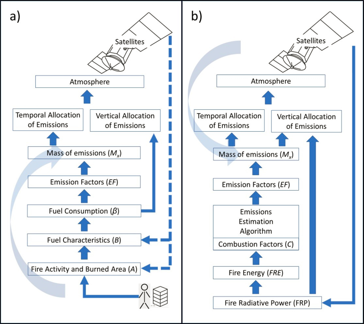
Andy Hudak, U.S. Forest Service, dove deeper into the bottom-up or activity-based approach for quantifying emissions from wildfires and highlighted opportunities for ground-based observations to reduce key uncertainties. The activity-based approach estimates fuel consumed either indirectly—based on fuel load estimates pre- and post-fire (Figure 12a)—or directly—based on observations of heat flux as fuel is combusted (Figure 12b) (French and Hudak, 2023). The largest contributors to uncertainties in emission estimates are (1) the process of consumption, which is highly variable; and (2) fuel beds, which are complex, heterogeneous, and challenging to measure on the ground (Larkin et al., 2012; Prichard et al., 2022). Burned-area maps from fire records or remote sensing are relatively better constrained.

Combustion accounting depends on many variables, including dead versus live vegetation and the amount of fuel moisture, which is coupled to soil moisture but more temporally dynamic, especially for fine fuel components such as senesced grass and litter that drive surface fire behavior as opposed to coarse woody debris and duff. Quantifying fuel beds is challenging due to their complexity. Remote sensing observations, particularly three-dimensional LiDAR (light detection and ranging) data, can provide information about fuel structure; however, the measurement sensitivity is mainly to the overstory canopy structure rather than the underlying litter and duff. Hudak explained that this is why large amounts of ground data are needed to capture the variability in fuels and burning conditions, which are key to understanding fire ecology, behavior, and effects. Hudak provided an example of using LiDAR measurements of the overstory to constrain estimates of litter inputs to a surface fuel bed, which can inform the ultimate goal of creating heterogeneous fuel maps (Sánchez-López et al., 2023). In addition to ground measurements of fuels, Hudak also noted the need for ground measurements of consumption from prescribed burn experiments. Prescribed burn experiments can provide multiscale data of how fuel types burn under different conditions (e.g., fire weather, fuel moisture) that can also be used to inform model estimates of emissions.

Hudak explained that the indirect approach using pre- and post-fire measurements has the disadvantage of not providing information about how fuel is consumed between the two points in time. Using a direct approach, such as heat flux during a fire, allows for estimates of how much combustion was flaming versus smoldering over the course of a fire—information needed to quantify the resulting emissions.

Jeff Vukovich, U.S. Environmental Protection Agency (EPA), described the bottom-up approach of the National Emissions Inventory (NEI) that quantifies emissions from anthropogenic sources, biogenic sources, and fires in the United States every 3 years. The NEI produces a day-specific emissions inventory of air pollutants, methane, and carbon dioxide (CO₂) for prescribed burns and wildfires. EPA receives activity data from states, localities, tribes, and federal agencies on a voluntary basis and combines that infor-

mation with satellite observations from the National Oceanic and Atmospheric Administration’s Hazard Mapping System.¹ To generate the inventory of emissions, the Smartfire2 tool is used to reconcile data sources and produce daily acres burned by fire type, and the U.S. Forest Service’s tool, Bluesky Pipeline, is used to estimate emissions for both flaming and smoldering phases (EPA, 2023). The NEI fire emissions are typically used for emission trend reporting, regulatory air quality and risk assessment modeling, and in research (e.g., air quality modeling). The Inventory of U.S. Greenhouse Gas Emissions and Sinks is a separate inventory produced at a national resolution each year.² Vukovich outlined a number of gaps and uncertainties in the NEI wildfire emissions, including activity data for prescribed fires, plume rise algorithms, methods to include pile burns, and emission factors. Vukovich also pointed to the opportunity to put more resources toward quantifying emissions in Alaska, particularly in non-NEI years when the fire activity may be high.

Quantifying Emissions from Satellite Observations

Louis Giglio, University of Maryland, discussed opportunities, limitations, and uncertainties for using satellite observations to understand wildland fire emissions. Satellites can observe many different parameters that can inform wildfire emission estimates, including

• Active fire presence: one or more fires actively burning within the footprint of a sensor;
• Fire radiative power (FRP)³: mid-infrared data show the presence of fires;
• Burned area: mapping cumulative area burned retrospectively;
• Land cover: classification of land cover types used as indicators of fuel type, or high-resolution fuel-specific maps; and
• Physical and meteorological parameters (e.g., fuel moisture, soil moisture, precipitation, etc.).

Giglio explained that satellite observations are the only practical way to comprehensively observe fire activity over the global biosphere. In general, the quality of satellite observations is improving and the data are generally freely available. However, the satellite data record is short compared to climate or human timescales. Additionally, the quality and consistency of satellite data vary over time and space, and the data are often stretched beyond their intended purpose to estimate wildfire emissions. Specifically, satellite observations of active fires and burned area can have omission (i.e., missed fire or burn) and commission (i.e., false fire or burn) errors, FRP observations can have errors in the analytical approximations used, and land cover classes can be misclassified.

___________________

¹ See https://www.ospo.noaa.gov/Products/land/hms.html.

² See https://www.epa.gov/ghgemissions/inventory-us-greenhouse-gas-emissions-and-sinks.

³ FRP provides an instantaneous burn rate, and fire radiative energy (FRE) is the time-integrated product of FRP and can provide the total biomass burned by a fire.

These uncertainties can all influence estimates of emissions; specifically, emission estimates can be overestimated or underestimated, systematically biased, assigned to the wrong time or place, or incorrectly attributed to fire or the wrong species. Further, uncertainties also depend on scale. Giglio identified the largest gaps or uncertainties facing the use of satellite data for quantifying fire emissions:

• Small burns that may be missed due to low spatial and temporal resolution,
• Limited diurnal sampling from polar orbiters,
• Less sensitive or spatially comprehensive sampling from geostationary sensors,
• Discrepancies in land cover datasets (e.g., Zubkova et al., 2023),
• Lack of long-term continuity and consistency across sensors and orbits, and
• Attention to quality assurance and validation.

Regarding key satellite observations needed to identify strategies to reduce GHG emissions from wildfires, Giglio said that forest and peatland fires are the most important from an emissions perspective, and that new and planned geostationary satellites, supplemented with polar orbiters at high latitudes, hold the most promise for observing these emissions with high frequency.

Drilling down into one example satellite observation, Martin Wooster, King’s College London, detailed the approach of quantifying wildfire emissions from FRP observations. The FRP approach for estimating fire emissions is the most direct approach that requires the least assumptions and can produce estimates of fire emissions in near real time, Wooster said. Imaging in the mid-wave infrared is sensitive to high-temperature sources, even if they are only a small part of a satellite pixel. Analysis of mid-infrared data allows for the presence of fires to be detected, including small fires observed at low spatial resolution. Observations are processed by active fire detection algorithms developed to be sensitive to the smallest possible fires while being insensitive to signals that are not fires. Generally, detectability scales with pixel area—in other words, if satellite pixels are 10 times larger in area, the minimum FRP that can be detected is 10 times larger. The FRP approach is considered a direct approach because ground measurements have shown that FRP is linearly related to the rate of fuel consumption. In practice, FRP data are converted into wildfire emissions using either a fixed conversion factor or derived relationships between fire radiative energy (FRE) and fuel consumption or smoke plume data (e.g., Kaiser et al., 2012; Nguyen et al., 2023).

Key uncertainties and challenges for the FRP approach include detecting cooler (e.g., tropical peat) fires, validation challenges due to rapid changes in FRP, atmospheric correction of observations, and conversion approaches of FRP to fuel consumption and emissions. Wooster sees opportunities in high-resolution geostationary satellites that can provide continuous observations. Regarding optimal spatial resolution for estimating emissions, Wooster’s work has found that 200-meter resolution is sufficient (Sperling et al., 2020).

Giglio explained that between FRE-based and inventory-based approaches, FRE-based approaches avoid the need for detailed information about fuels but require high-

frequency temporal sampling; inventory-based approaches require detailed information to estimate what fuel burned, but do not require as high a resolution for temporal information.

Hybrid Approach for Quantifying Emissions

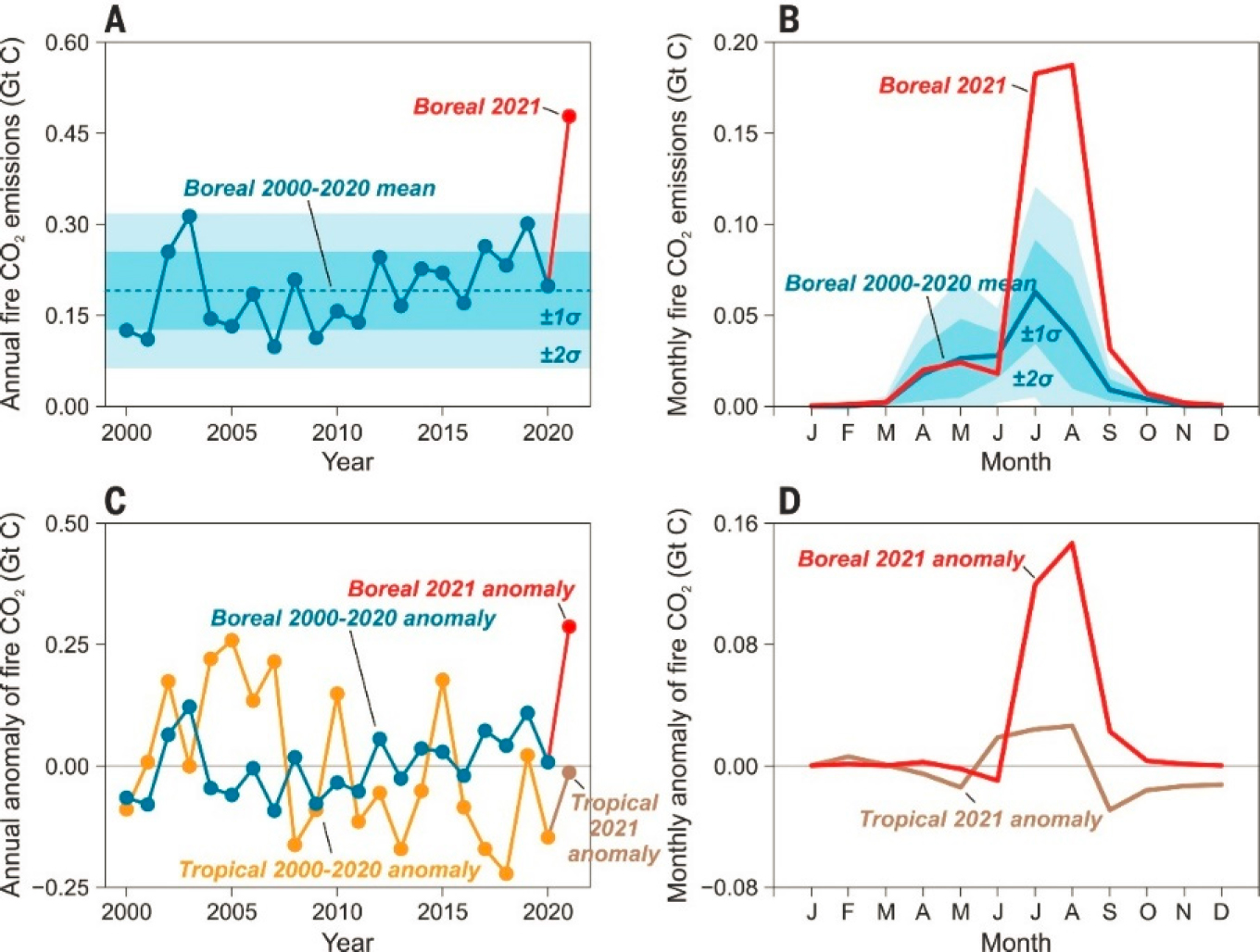
Zheng showed a hybrid approach for quantifying emissions that combines both activity-based and atmospheric-based approaches to estimate carbon monoxide (CO) and CO₂ emissions from fires. In Zheng’s approach, he uses satellite observations of CO—an important tracer for smoke from wildfires—to constrain CO₂ emissions using an inverse model (Zheng et al., 2018a, b). Then, he uses CO emission factors to derive combustion efficiency, which determines how much carbon, or CO₂, is released from fires globally (Zheng et al., 2021). Using this approach, Zheng has found that globally, burned areas have decreased since 2000 while fire emissions per unit area burned have slightly increased (Zheng et al., 2021). This hybrid approach allows for investigation of these trends; the decrease in burned area globally was due to declines in grassland burning while emissions from forests have increased, primarily in boreal regions where emissions increase when there are high water deficits (Figure 13) (Zheng et al., 2023).

Challenges in Quantifying Emissions from Prescribed Fires

Morgan Varner, Tall Timbers, focused on key uncertainties and challenges in quantifying emissions from prescribed fires. Prescribed fire is not monolithic; it includes a diversity of fuels, fire behavior, and emissions. In the United States, the largest area where prescribed burning happens annually is in the Southeast, where it is used primarily for biodiversity conservation and wildlife. Varner noted that compared to wildfires, prescribed fires are underrepresented in terms of research funding and attention in scientific publications. Varner reiterated that key uncertainties for understanding emissions from prescribed fires are the spatiotemporal heterogeneity of fuels, fire behavior, and resulting fuel consumption. Estimating the quantity, location, and timing of prescribed burning in the United States is challenging, whether the data are coming from state forestry agencies or satellites (e.g., Cummins et al., 2023; Melvin, 2022; Vanderhoof et al., 2021). For example, permit data for prescribed fires in the United States are an imperfect metric. Permits only capture an estimate of the acres that will be burned; these data are not updated based on how much was actually burned, and the data collected vary state to state. Regarding the use of satellite data to quantify emissions, it is difficult to attribute observations to prescribed burning versus wildfires or agricultural burns.

Varner highlighted the importance of scale for detecting variations in consumption and fire effects, including the heterogeneity at the stand scale (Kreye et al., 2020). There are large uncertainties in characterizing fuels in fine-fuel-driven systems, including for solid fuels such as duff and peat. For example, although duff is an important generator of emissions, it is spatially patchy, and more work is needed to improve predictive models, Varner said. There are also large uncertainties in prescribed fire behavior that have complex, intricate ignition patterns unlike large wildfires. Breakout discussions also noted the lack of data on the effects of prescribed fire on subsequent fires (Box 4).

MODELING EMISSIONS FROM WILDLAND FIRES

The second session of day 2 provided an overview of different approaches for modeling emissions from wildland fires. Specifically, speakers focused on simulating fire in global dynamic vegetation models and lessons learned from the Fire Modeling Intercomparison Project (FireMIP), modeling forest fire interactions in the western United States, statistical methods for defining global pyrogeography and pyromes, and regional-to-global projections of fire emissions.

Global Fire Models

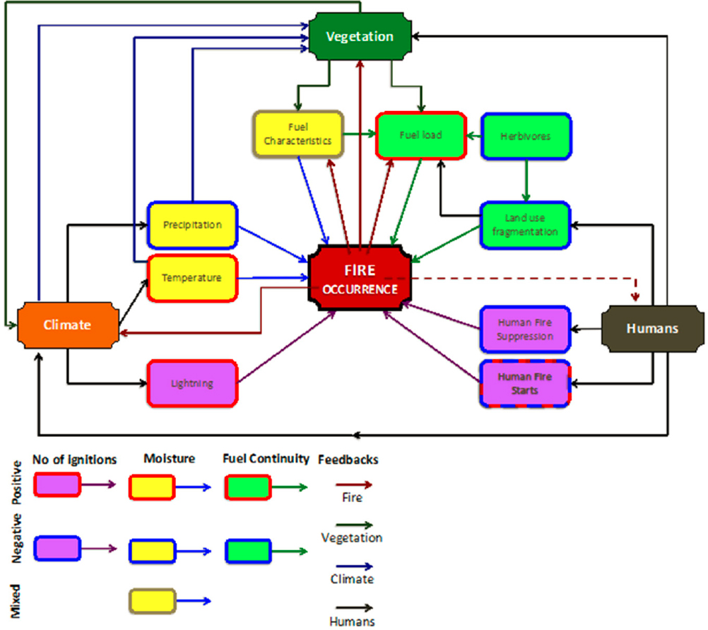
Stijn Hantson, Universidad del Rosario, introduced global fire modeling and presented several example applications. Fire models aim to represent the main drivers of fire occurrence, including the climate, vegetation, and human drivers (Figure 14). A key consideration for models is how they represent the interactions between the various drivers.

For example, if a fire model is not coupled to a vegetation model, it cannot capture the interactions and feedbacks between climate change and vegetation status or the feedbacks of fires on vegetation. Dynamic global vegetation models (DGVMs) are critical for incorporating these processes into global fire models, Hantson said. DGVMs simulate ecosystem processes based on a simple set of input parameters (e.g., sunlight, CO₂, soil properties) (Prentice et al., 2007). Fire influences all of these ecosystem characteristics, for example, tree mortality and competition between species, among others. DGVMs provide fuel loads and ecosystem status as dynamic inputs to fire models.

Hantson described two main categories of global fire models. One type is the simpler empirical global fire model that simulates a global pattern of burned area based on empirical equations with inputs such as climate drivers, fuel characteristics, and impacts of humans. The second type is the process-based global fire model that simulates the chance that ignition will turn into fire, and when an individual fire occurs, how fast it spreads, and how much area is burned. This individual fire behavior is then upscaled to represent a global pattern of burned area. There is a range of global fire models that have large variations in their inputs and parameterizations and which processes are accounted for, but all models produce estimates of burned area (Rabin et al., 2017).

FireMIP grew out of the need to methodically evaluate the capabilities and uncertainties of existing global fire models (Hantson et al., 2016; Rabin et al., 2017). FireMIP was a community effort to analyze and benchmark the existing global fire models and systematically understand and decrease uncertainty in global fire model projections. Comparing how models simulate global burned area and fire emissions, models generally reproduce the global pattern, with most burning across tropical savannas (Hantson et al., 2020). Seasonality in burned area and fire carbon emissions is also generally well represented by the models, with peak burning better represented than the length of the fire season (Hantson et al., 2020). Hantson also showed a study that used a global fire model to compare burned area changes under climate change from reanalysis data with another dataset without climate change and they were able to show that climate change has increased present-day global burned area by 16 percent (Burton et al., 2023).

The DGVMs generally also reproduce observed relationships with climate variables, but models have trouble representing the impact of changes in previous-season plant productivity and increasing burned area, which may explain why models struggle to represent interannual variability (Forkel et al., 2019). As one example of how limitations in vegetation models impact global fire models, vegetation models have a hard time representing soil organic layers, which if not simulated, cannot then be combusted in a global fire model and may lead to large underestimates in carbon emissions, for example, in boreal North America.

Approaches for Understanding Regional Fires

Park Williams, University of California, Los Angeles, focused on modeling forest fires in the western United States. One of the main drivers of the increase in annual area burned in forests is the warming and drying of the atmosphere. Vapor pressure deficit—the difference between the amount of moisture in the air and how much moisture the air can hold when it is saturated—has increased with increasing temperature, and there is a strong exponential relationship between vapor pressure deficit and burned area (Juang et al., 2022). However, Williams explained that the future will be more complicated than simply extrapolating this historical exponential relationship.

Williams showed results from a new statistical wildfire model for the western United States that responds to changes in daily climate variables (e.g., vapor pressure deficit, precipitation), ecosystem variables (e.g., forest biomass), and human variables (e.g., distance from populations) and generally represents observations of regional and seasonal variations in area burned. When their statistical model is applied to the historical and future period without coupling between the fire and dynamical vegetation model, the statistical model predicts an explosion in area burned by the end of the century. However, ecosystems are critical for regulating area burned; forest fires can have a self-regulating effect in which subsequent fires do not burn as large or intensely through an area that has burned recently. At the subcontinent scale in the western United States, the degree to which annual area burned will increase in the future may be strongly influenced by the self-regulating impact of forest fires (Abatzoglou et al., 2021; Turco et al., 2023).

Complex models are needed to make future predictions about forest fires in the western United States, explained Williams. A mid-range (i.e., 1 kilometer) forest ecosystem model—for example, Dynamic Temperate and Boreal Fire and Forest-Ecosystem Simulator (DYNAFFOREST)—is an example of a compromise between landscape-scale and global-scale models (Hansen et al., 2022). When Williams couples his statistical fire model with the DYNAFFOREST ecosystem model, by the end of the century, while fires are still large, they are about 15 to 20 percent smaller on average due to this self-regulating impact, compared to the uncoupled model. Beyond area burned, this self-regulation also leads to approximately 20 percent less carbon burned per area compared to the 20th-century mean.

Regional fire modeling is relatively nascent, and Williams identified a number of major limitations:

• Simple representations of fuels do not yet include the effects of ladder fuels, ecosystem types other than forests, or insects and diseases;
• Effects of prior or subsequent burning (i.e., self-regulating behavior) are difficult to validate;
• Observations of biomass combusted to validate regional models are limited;
• Simulations of alternative management approaches are challenging because models have been developed on data from the suppression era;
• Uncertainty exists in the effects of CO₂ fertilization on forests;
• Expertise across disciplines can be beneficial to partner in large teams; and
• Computational resources are important to support the coupling and high resolutions for future projections.

Williams argued that modeling wildfire at the regional and continental scale would require a large investment in resources, similar to historical investments in global climate modeling.

Matthew Jones, University of East Anglia, showed new work on regional mapping that reveals shifts in the global geography of forest fires. Archibald et al. (2013) applied clustering analysis to observations of fire characteristics in order to group different parts of the world with similar fire characteristics, defined as global pyromes. These pyromes are useful for studying fire regimes, but they do not provide information about what these pyromes are sensitive to—for example, climate change, land use change, or changes in vegetation productivity.

To address these limitations, Jones introduced “pyronia”⁴—regions with similar fire controls, including climatic factors (e.g., soil moisture, fire weather index), vegetation factors (e.g., fuel stocks), and human factors (e.g., population density, cropland cover). Clustering analysis—a machine learning approach—was used to identify regions where forest burned area has similar sensitivities to the wide range of potential controls on fire. Machine learning techniques can be a “closed box” that requires disentangling to understand and

___________________

⁴ Note: Pyronia is also a genus of butterflies; in context of this proceedings, pyronia refers to regions with similar fire controls.

interpret the results. Jones showed how the distribution of correlations across ecoregions within each pyronia can provide insights about what the clustering algorithm identified as unique about each pyronia. For example, Jones’s analysis showed that extratropical pyronia in the temperate and boreal forests are sensitive to fire weather and/or drought and are not sensitive to human controls (e.g., land use, human ignitions).

Once these pyronia have been identified, they can be used to explore how fire behavior has changed in recent decades. Jones showed an increase in burned area, fire severity, and ultimately carbon emissions in the extratropical and suppression zone (i.e., regions where fire suppression has been a dominant forest management practice) pyronia, and decreasing burned area, severity, and carbon emissions in the tropical and subtropical forests. Jones noted that while this approach did not utilize a global fire model, there are ways the two modeling approaches could complement one another—for example, global model parameterizations could be defined or tuned to each pyronium.

Projecting Future Fire

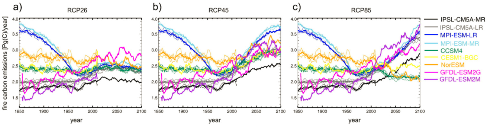
There is growing interest in making projections of future fire to understand a range of risks including meteorological risk, burned area, and carbon emissions. In a comparison of Earth system models that simulate fire, Kloster and Lasslop (2017) showed that there is wide variation in how these models simulated burned area in the late 20th to early 21st centuries, both compared to each other and against observations. Jed Kaplan, University of Calgary, argued that global fire models are not successfully representing fire and that more work is needed in this space. Global fire models show large variations in representations of carbon emissions in the past, a convergence in the late 20th and early 21st century due to model tuning to independent estimates of fire emissions, and divergence in their projections of fire emissions in the future (Figure 15) (Kloster and Lasslop, 2017).

Kaplan elaborated on the differences between model projections of the future by showing experiments that used one fire vegetation model together with different global climate models and future emission scenarios. Climate model simulations of burned area and fire carbon emissions in both the recent past and end of century are different, indicating large uncertainties (Koch and Kaplan, 2022). Examining the spread of models shows that while there are large differences in the magnitude of carbon emissions depending on which meteorology the fire model uses—indicating a model bias—the models generally simulate similar trends, mainly because the models are driven by the same GHG emission scenarios in which there is a direct effect of CO₂ on vegetation and an indirect effect of CO₂ on climate (Koch and Kaplan, 2022).

Kaplan outlined major drivers of uncertainty for projecting future fire: (1) simulated meteorology, (2) fuels and their structure, (3) spatial resolution and landscape heterogeneity, and (4) “anthropogenic fire” or how people use fire today. Regarding uncertainties in anthropogenic fire, Kaplan pointed to the Global Fire Use Survey, an international effort to map the ways humans interact with fire on the present-day landscape. Regarding gaps in measurements, Kaplan reiterated comments from other speakers on the need for data on fuels, particularly in developing countries; future land use projections, particularly related to fuels management and anthropogenic fire; and observations of small fires, particularly as part of smallholder land management. Additional opportunities to improve model estimate of GHG emissions from fires are noted in Box 5.