Transit Traction Power Cables: Replacement Guidelines (2024)
Chapter: 2 Answers to Key Questions

CHAPTER 2
Answers to Key Questions
2.1 Useful Life of Cables
Existing transit systems vary in age and size, and they can be classified as small, medium, or large. In this guide, different types of transit systems are investigated. The lifespan of cables is affected by electrical parameters such as jacketing, cable size, diameter, the method of insulation, whether they are overhead or underground, operating voltage, and weathering. Several attempts have been made to determine the factors associated with the influence on the life cycle of wire and cable insulation and jacketing. Zhou et al. (2017) conducted an in-depth analysis of the research and development of cable failure analysis, condition monitoring and diagnosis, life assessment methods, fault location, and optimization of maintenance and replacement strategies. The findings showed that the proportion of joint failures, termination failures, and cable body failures was 37%, 32%, and 31%, respectively. Most partial cable failures occur in a joint where splices have been improperly placed to repair a previous cable failure. As such, it is imperative that cable repairs are executed correctly (Silva 2012). Over the years, developments in technology have led to better-insulated cables, as shown in Figure 2.1.
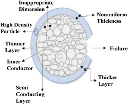
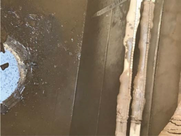
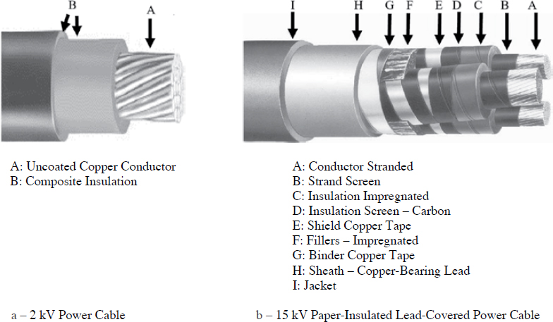
Manufacturing defects, poor workmanship, and external damage are significant causes of cable failure. Failure brings various consequences related to medium-voltage (MV, rated at 10 kV to 20 kV) distribution cables and transmission cables. Other factors that result in cable failure are poor installation of cable accessories, poor manufacturing of cable bodies, and aging factors. Thermal, electrical, mechanical, and environmental stresses can act singly or synergistically on cable insulation defects (Aldhuwaian 2015; Reid et al. 2013). Research suggests that the average life of high-voltage (HV) cables is 13 to 18 years, while the expected life of MV cables is approximately 20 years (Levi and Shah 2018). In Figure 2.2, the typical construction of an MV cable is shown. An underground insulation material chart is shown in Figure 2.3, and a poor design example is shown in Figure 2.4.
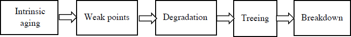
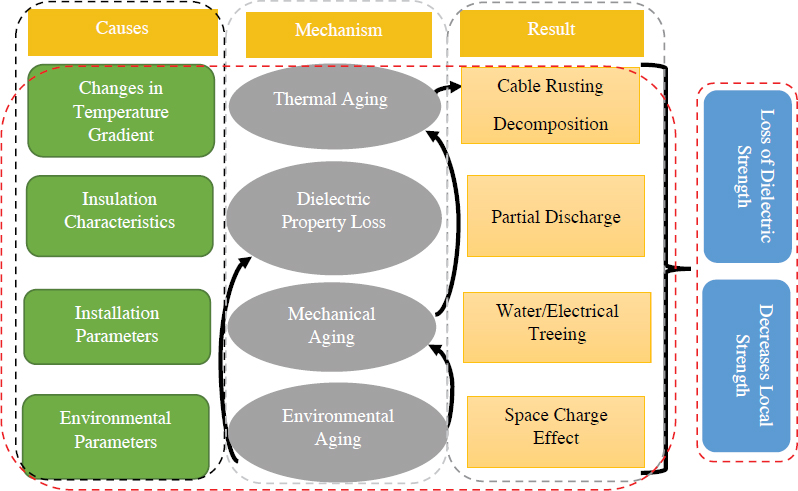
Research shows that there are relationships between detection, distance covered by the transit system, and the weather. Older transit agencies use physical detection to find damage to their cables. Therefore, most of their inspections involve physical detection of the faults. Modern transit systems continuously check cables and fix them immediately when a fault is detected. Various electrical types of equipment are involved, which measure conductor loss, insulation loss, rise in resistance values, and other factors to find damaged cables (Altamirano et al. 2010; Densley 2001). In Figure 2.5, a pattern of the breakdown of cables is given. In Figure 2.6, cable aging, mechanisms, and consequences are shown in a flowchart.
Aging is the irreversible degradation of properties, and it affects the behavior and performance of cables as well as cable service life. The growth of water trees in insulation systems plays an important role in cable degradation. Water trees are dendritic patterns with branching through
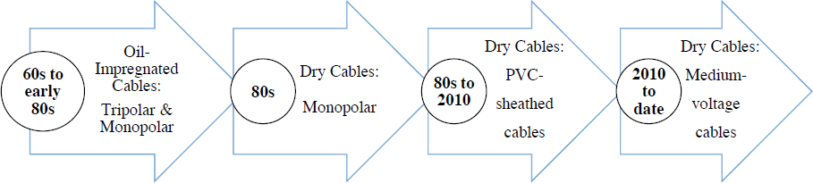
Figure 2.1. Worldwide cable technology change over the years.
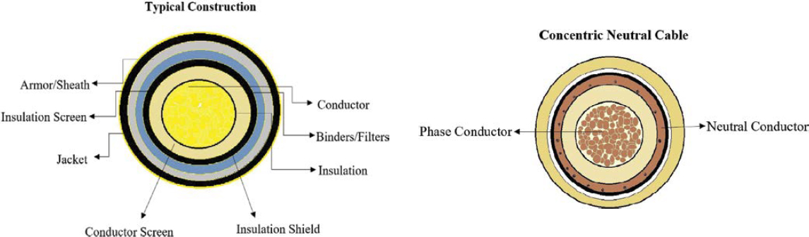
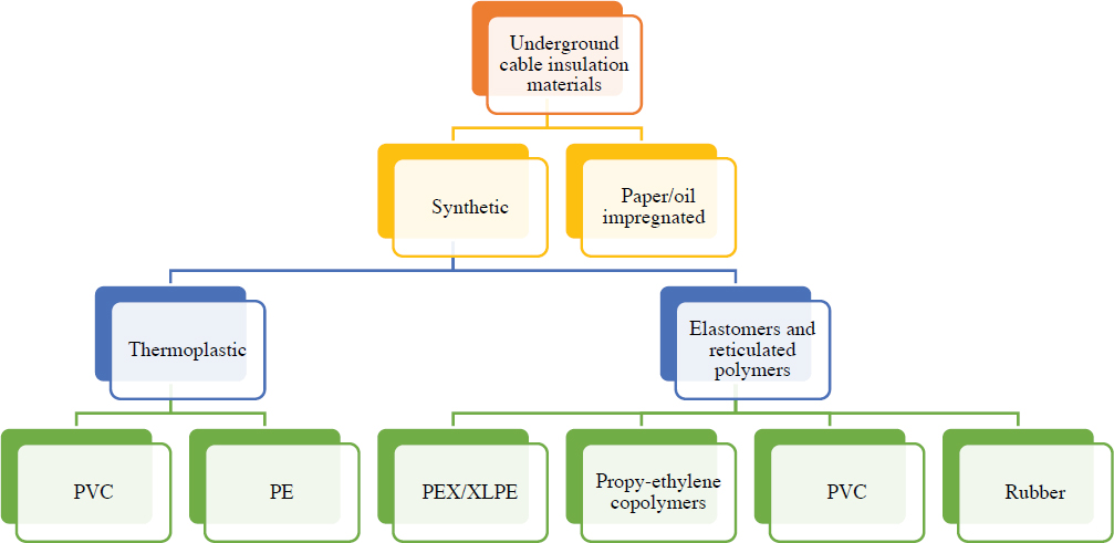
Figure 2.3. Underground insulation material chart.
the walls of insulation that grow in hydrophobic polymers in an alternating current (AC) electric field and water (Terezia 2013). They are formed from water molecules introduced into the insulation from either manufacturing processes or from the outside environment. The water molecules usually flow aimlessly throughout the insulation.
Water trees form due to an area of high electrical stress typically caused by another defect and are often found in areas in the cable in a state of tension, such as a bend. Often, water treeing is invisible to the human eye, but special dying techniques can make water treeing more visible. According to Mashikian and Szarkowski (2006), water treeing will not create a fault in the cable, even if they are present through the entire insulation (Neimanis et al. 2004; Terezia 2013).
Electrical trees are similar in appearance to water trees, yet their occurrence and formation are different. Water trees form over time when moisture is present in the insulating material. Electrical trees can be caused by voids, impurities, defects, or a combination. Most often, they occur in locations of high electric stress. High electric stress on AC cables will often accelerate the formation and growth of electrical trees compared to low-stress cables (Laurent et al. 2013). Electrical trees can be grouped into two broad classifications: vented and bow-tie trees. Typically, vented trees progress more quickly than bow-tie trees because they do not have as large a partial discharge or disruption of the electric field associated with them. Electrical trees can cause partial discharge, which can be picked up by different kinds of diagnostic tests, and they are usually visible to the naked eye if within the insulation (Lanz and Chatterton 2018; Dodds 2017). Professionals sometimes believe that electrical trees are nearly impossible to catch with testing because once they form, failure is quick to follow. However, there is evidence to the contrary. Cable failure depends on several factors. If a water tree is present, it can hinder the growth of electrical trees (Laurent et al. 2013).
Another reason for faults is when foreign objects inside underground cable systems enhance stress. A foreign object that makes its way into the insulation due to improper installation can change the distribution of the electric field, causing a higher stress area in situ (Lanz and Chatterton 2018).
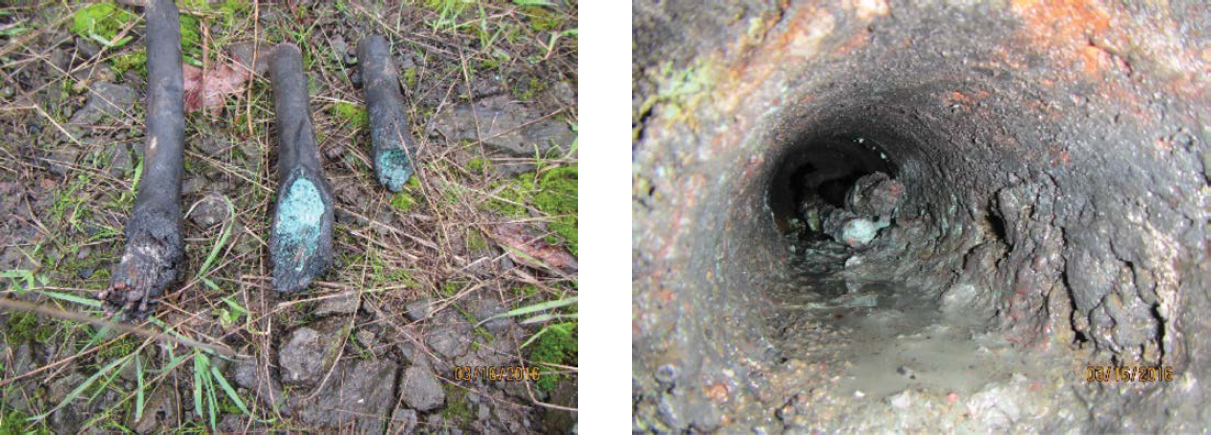
Corrosion is the main reason for cable rusting decomposition and failure. It may also lead to other defects that can cause failure. The metal part of cables can last underground for an incredibly long time. Polymer as an insulation may thermally or chemically break down over time. The insulation material has a long half-life. Cable components that do not corrode, such as cable tape shielding, impede water migration and can delay or prevent corrosion. Most cable insulation is chemical resistant by specification. Any area of cable exposed to corroding agents such as running water or chemicals can lead to issues in the cable (Dodds 2017; Gregorec and Ideal Industries, Inc. 2004). Examples of cable failure from corrosion are shown in Figure 2.7.
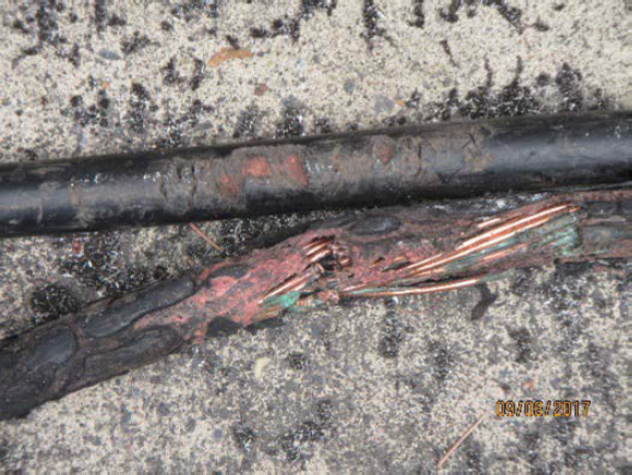
Overheating is another agent that can affect underground cable systems. Overheating commonly occurs in cable joints. Cable temperature depends on the conductor and dielectric losses; installation environment, such as water, ground, and air; the thermal conductivity of the cable and surrounding material; ambient temperature; and other external sources of heat (Lanz and Chatterton 2018). Overloading due to excessive electrical current flowing causes overheating. External heat rarely damages a cable, unless it is from a fire. One of the most common yet most preventable agents of cable faults is installation errors. Numerous errors can be seen in installed underground cable systems, and many of them can take years before occurrence of a fault. Electrical arcs can occur when two conductors of separate circuits make contact. Arcing may cause burning to occur (Lanz and Chatterton 2018). Figure 2.8 shows an example of cable failure. Figure 2.9 presents common installation errors. Figure 2.10 presents sectional problems on installed cables.
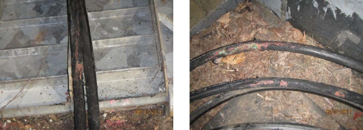
Many potential issues resulting from poor installation or other factors may take years to occur or may never happen. Often, when a fault does occur, it is accompanied by an arc flash or explosion. An arc is where the charge jumps an air gap from the underground cable to a surrounding material or a cable to complete a circuit (Neier et al. 2019). Figure 2.11 shows some examples of cable failures.
Some actions that can be taken to enhance the useful life of underground cables are to consider (1) preexisting contamination and water bodies, and (2) landscaping, stormwater paths, planting, and any other disruptions in the underground lines when choosing the cables routes. Water bodies may cause erosion around the cable lines, which may lead to leakage into the cables. Developing proper land surveys and having agreements to control landscaping and stormwater paths may provide protection to underground cables, thereby avoiding malfunction (Barron et al. 2017).
2.2 Degree of Degradation
One of the most prevalent causes of degradation in cables is changes in weather conditions, air moisture, and temperature. Research conducted by Hyvoonen (2008) predicts the insulation condition of MV cable insulation. Different electrical measurements and chemical analyses are performed to find the most representative combination. A large-scale test program was carried out on field-aged and oil-impregnated paper-insulated cables. Methods such as dielectric response measurement and Fourier transform infrared (FTIR) analysis were used to determine the degree of degradation. Hyvoonen (2008) found that the cables used were still in good condition after 30 years of service. The FTIR-analysis results had a good correlation to the voltage withstand levels of the cable samples. The various degradation parameters used in the experiment consisted of chemical degradation, free radical formation, polymer radical degradation mechanisms, thermal and electrical degradation, water treeing, and electrical treeing. Figure 2.12 presents examples of traction power cables.
Chang et al. (2018) present a predictive model of the degradation of cable insulation subject to radiation and temperature. The method developed in the study is a novel degradation model that has been cited by various researchers. According to the research, with aging, elongation at break (EAB) of the insulation gradually decreases as a function of time. According to the model,

The virtual degradation rate is determined by fitting experimental data with physics-based equations. The study conducted on aging mechanisms and monitoring of cable polymers by Bowler and Liu (2015) demonstrates that aging-related changes in the insulation material’s dielectric properties can be monitored using a capacitive sensor. The cable capacitance and dissipation factor can be measured in situ on samples using a clamp capacitor adapted for the cable dimensions of interest. Alternatively, sensing patches can be permanently placed and periodically excited via the applied voltage across contact pads. One potential advantage of the
EAB before and after aging is related to the amount of the virtual degraded part to the power of one-third. The amount is modeled by the cumulative distribution function (CDF) of exponential distribution at a fixed virtual degradation rate. This CDF represents the amount of the yield as a function of the virtual degradation rate and time.
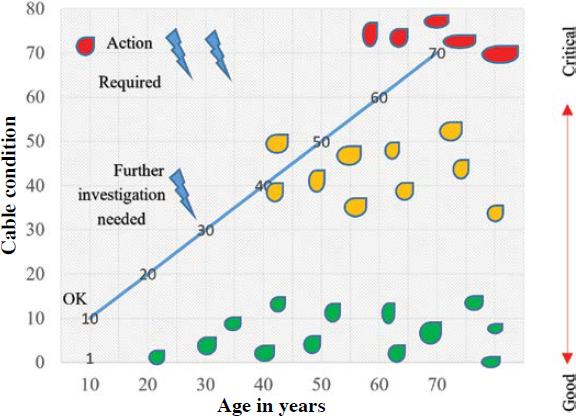
capacitive sensing by permanently placed electrodes over mechanical property measurements by an indenter is the capability of in situ monitoring. The method of degradation measurement used permittivity of polymers and the dielectric and mechanical measurements on aged wire insulation. The research suggests that in conjunction with identifying new indicators of polymer aging, the proposal of a new acceptance criterion for cable insulation based on voltage breakdown rather than EAB has been considered (Neier et al. 2019). In Figure 2.13, the distribution of cable conditions is given over the years. There are three stages in the graph. The first one is marked in the graph as “OK,” the stage that does not need any action; the second one needs further investigation. For the third one, action is required.
Szatmári et al. (2015) studied underground cables for 5 years to determine the degradation of cable insulation jackets. According to the researchers, the degradation process starts with the deterioration of the outer polyethylene layer, which can be prevented by cathodic protection against the cable metallic screen corrosion. Research was carried out with experimental and analytical investigations, and the study compared experimental and analytical investigation results.
2.3 Detecting Degradation of Cables
Based on the size of structures and the type of power supply of various transit agencies, there are vast numbers of indicators that can be used to test and verify the aging of cables. One of the most common techniques is cable monitoring (CM), and it detects damage and measures the extent of degradation in electric cable insulation. Factors considered in selecting appropriate CM inspection guidance include intrusiveness, cable characteristics, and degradation mechanisms. Commonly used condition monitoring techniques include visual inspection, compressive modulus testing, dielectric loss measurement, insulation resistance testing, polarization index, AC voltage withstands testing, partial discharge testing, direct current (DC) high-voltage testing, step voltage testing, and time-domain reflectometry testing. The various test result reports suggest the applicability of various diagnostic indicators to monitor cable condition. The occurrence of cable failures, often before the end of the original specified lifespan, has shown that functional testing alone does not fully demonstrate the capability of a cable circuit to perform its function under all normal and abnormal operating conditions, since it does not fully characterize the condition and dielectric integrity of the cable’s insulation system (Nowbakht et al. 2015). A health monitoring index (HMI) tool was introduced by Meijer et al. (2015) to assess a cable system’s health and evaluate maintenance strategies. In the HMI, the data were obtained through transfer functions based on cable data; three types of assessment functions (statistical, condition assessment, and prediction) were applied to each of the cable attributes to produce assessment results; after translating the assessment results by folding functions, HMI indicators were produced to determine the remaining lifetime of the cables.
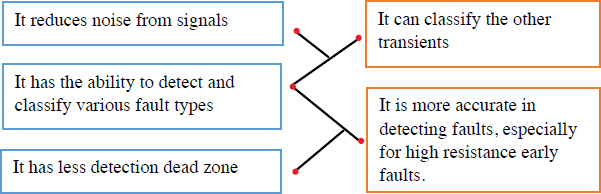
Sidhu and Xu (2010) studied the initial defects in underground cables and proposed a scheme for early detection of underground cable faults. Figure 2.14 shows the main advantages, found in the study, of an early detection system for underground cable faults. The system was tested on an underground cable model for two different cases. The primary case indicated a shorter life expectancy than the design lifetime, unlike the second case. The estimated results obtained were close to actual values. The outcomes showed that loading condition was the main factor in determining the lifespan of cables.
Sachan et al. (2016) used the degradation level and failure distribution of cables to develop a probabilistic dynamic programming model to determine the optimal maintenance policy for cables. This optimal policy recommends timely preventive maintenance and replacement decisions. This probabilistic model can also assess the imposed financial risks.
Another approach found in the literature for defining degradation is the partial discharge (PD) diagnosis method. This diagnosis indicates weak spots in a cable connection. To run the measurement, partial discharges are ignited in the cable insulation or joints by applying a test voltage. Orille-Fernández et al. (2006) used artificial intelligence and artificial neural networks (ANNs) to predict failure risk due to lightning surges in a range of ground MV cables up to 30 kV while considering the cables’ different insulation levels. The ANNs can be used directly
to estimate the failure risk for a specific network or indirectly to decide which kind of lightning arrester, maximum cable length, or cable insulation level must be used to reach a particular failure risk. Partial discharges have physical characteristics and are described by parameters such as PD inception voltage, PD pulse magnitude, PD pattern, and PD site location in a cable. Another method discussed is tan δ measurement. This can be applied to determine the loss factor of insulation material. This factor increases during the aging process of the cable. Outcomes of degradation are shown in Table 2.1.
An experimental study carried out by Kauhaniemi et al. (2019) investigated cables with two PD sources at various places. The authors proposed that the wave propagation velocity of the cable be determined experimentally to enable locating the PD faults with increasing accuracy. Time-domain-reflectometry–based measurement methodology was applied on single-end measurements using the high-frequency current transformer sensor installed at one end of the cable. The study describes the methodology for two PD sources. If several PD sources are present at several locations, a discussion is presented to implement an “automated” monitoring system based on the principles of the proposed technique.
Zhang et al. (2021) proposed a strategy of using infrared temperature estimation. The authors analyzed thermal probability density (TPD) regularities to gauge the sort and degree of inside cable deficiencies, based on a three-dimensional electromagnetic-thermal multiphysics show of control cable. When internal cable faults occur, the dispersions of surface temperature probability density curves are different. By combining the TPD’s characteristics, a comprehensive judgment can be made to accurately determine the type and degree of cable defects. Also, an experimental platform was built to verify the system the authors proposed. The experimental outcomes were consistent with the simulation outcomes, demonstrating the method’s feasibility.
Ocuon et al. (2015) conducted thermal examination of an underground cable system. An in-line course of action of cables was considered. Computations were performed using the finite element method (FEM) code created, as shown in Figure 2.15.
A study carried out by Ocłoń et al. (2015) addressed the application of momentum-type particle swarm optimization for the thermal performance optimization of underground cable systems. Thermal performance optimization of an underground cable system was presented. An electrical energy transmission line that consists of three underground cables, placed in a flat (in-line) arrangement, was considered. Kruizinga (2017) presented research for underground cables. Due to the low impact on the average amount of customer minutes lost in the low-voltage (LV) grid, this grid level has long been neglected in the optimization process of asset management. However, due to the number of outages, the costs of repairs are relatively high. Currently, the replacement of grid sections only takes place after repeated outages in the same section because there are no methods available to perform diagnosis on LV grids.
Table 2.1. The outcomes of degradation.
| Compliance with industry standards is very important for quality assurance. | Breakdown strength stability can be determined using retained AC breakdown tests. |
| Compatibility of extruded core materials for cables is important to provide high standards. | Relative ranking of similar types of insulations. |
| Insulation should provide water-tree resistance. | Distinctions between insulations can be more easily seen at a higher stress/lower temperature than at higher stress/high temperature. |
| Operating conditions are very important for cable life. | Insulations with equal life performance cannot be distinguished using accelerated cable life testing. |
The characteristics of cables permit them to be fixed after failure. It is important to use the strategies outlined for repairable frameworks for modeling cables’ lifetimes. In the research of Nemati et al. (2019), the effects of control cables’ reparability characteristics on failure rate estimation are displayed, and data-driven approaches are used to take advantage of databases already available at many power distribution companies to extract the required information. The circumstances considered in this work are age, type of conductor, length, joints, the length of insulation cables compared to the total length of a feeder line, and geographical location.
Once degradation occurs in cable, a failure of some degree will occur. Once a cable fails, agencies decide to replace or repair the cable. Another decision for agencies to make is when to replace a cable due to its age. Testing is a useful and valuable tool for establishing the overall scope and priority within a cable replacement program by comparing cables within similar groups. Testing can also be the answer if an unscheduled outage has occurred as to whether the global condition of the cable insulation warrants an economically justifiable repair. This is called a “repair-or-replace” decision.
2.4 Factors Influencing the Lifespan
Cables are critical assets for transit systems, and cable lifetime is generally estimated from the temperature change and associated lifetime reduction. However, determining lifetime reduction is intricate due to the complex physics-of-failure (PoF) degradation mechanism of the cable. This is further complicated by other sources of uncertainty that affect cable lifetime estimation. Generally, simplified, or deterministic, PoF models are adopted, resulting in non-accurate decision-making under uncertainty. In contrast, the integration of uncertainties leads to a probabilistic decision-making process affecting the flexibility to adopt decisions. The lifespan of cables used by transit agencies varies based on the cables’ specific properties. Sutton et al. (2010) describes the various environmental factors that influence the lifespan of cables. According to this study, the lines are so durable that the electrical towers and insulating systems are more likely to fail over time than the lines themselves. Lines are generally not replaced unless the electrical voltage levels in a certain transmission area need to be increased.
Factors influencing the lifespan were discussed. In Jones and McManus (2010), 30-year net present value analysis of the economic feasibility was conducted to compare the cost of the two types of the cables. The economic feasibility evaluation and simulation study results helped determine the appropriate types of cables. The authors defined the life-cycle effects of different types of electrical cables. A total of five types were analyzed—three overhead lines and two underground cables—and were compared based on factors affecting lifetime operational procedures. Useful life of underground cables is affected by various parameters, such as surrounding
temperature, the depth of the laying of cable, the number of parallel circuits of cable, and the encompassing soil’s thermal resistivity. Gouda et al. (2009) presents an experimental work related to the dry-zone phenomenon linked to various parameters affecting underground cables. Neier et al. (2019) focused on one of the key questions related to factors influencing underground cables: how to estimate the remaining lifetime of underground cables? After weak spots are cleared, the general aging condition of the cable can be judged, and the remaining lifetime can be estimated. A tool for asset managers was included that is expected to assist in developing a preventive maintenance approach.
Aizpurua et al. (2021) developed a novel cable lifetime estimation framework that connects data-driven probabilistic uncertainty models with PoF-based operation and degradation models through Bayesian state-estimation techniques. This framework estimates the cable health state and infers confidence intervals to aid decision-making under uncertainty. The proposed approach is validated with a case study with different configuration parameters, and the effect of measurement errors on cable lifetime is evaluated with a sensitivity analysis. Results demonstrate that ambient temperature measurement errors have a more significant influence than load measurement errors. The greater the cable conductor temperature, the greater the influence of uncertainties on the lifetime estimate.
Neier et al. (2019) provided an approach to estimate underground cables’ remaining life. This approach depends on defining the weak points in cables by combining tan δ and PD diagnostic methods. Accordingly, the general aging condition of the cable can be judged, and the remaining life can be estimated.
Zawaira et al. (2017) proposed a power transmission line model. It combined wavelets and the neuro-fuzzy technique for fault location and identification in underground cables by extracting certain features of the wavelet transformed signals to develop an adaptive neuro-fuzzy inference system (ANFIS) for fault location. With a precision of 99.6%, the ANFIS managed to locate the fault. ANFIS output was evaluated for fault position, and results were obtained. Finally, it was shown that the proposed wavelet-ANFIS technique-based approach for underground cable fault location was reliable enough to be used in the detection of transmission line faults.
Metwally (2011) discussed preventive maintenance techniques for cables. Examples of these techniques are dissolved gas analysis, partial discharge measurement, thermal monitoring, capacitance and loss tangent (dissipation factor), and frequency response analysis.
Kroener et al. (2014) studied heat dissipation in underground cables, cable lifetime, cable temperature, and the properties of the surrounding soil. The lifetime of an electrical underground transmission line system is very sensitive to both average temperature and fast changes in temperature. Incorrect estimates of the cable’s temperature can lead to severe errors in the estimated lifetime. The coupled model for heat dissipation, liquid water, and vapor transport in soils was tested by adding an impermeable layer below the cable and by keeping the water content around the cable, the thermal conductivity, and the heat capacity higher. Numerical simulation under real weather conditions revealed on one hand that seasonal air temperature defines the seasonal evolution of cable temperature. At the same time, precipitation is strongly related to changes in cable temperature on a time scale of hours to a few days. Simulations under consideration of additional structures (concrete slab, impermeable V-shaped layer, silt layer) showed that these simple test cases can reduce average temperature and variation of temperature by some degrees, and in this way increase the system’s lifetime compared to a homogeneous example.
Kroener et al. (2014) demonstrated that during the construction of an electric underground transmission line system, it is fundamental to consider the coupling of liquid water, vapor, and heat flux to estimate the temperature and expected lifetime of the system. The thermal processes are strongly influenced by weather conditions. Therefore, it is important to compare the
differences among various weather conditions at different sites and in different years. In general, a correct simulation provides a better design of cable installations. Experimental tests help in choosing the correct cable specifics, the installation depth, and the surrounding backfill. The choices may change depending on the properties of the natural soil and the weather conditions. Overall, this model holds potential for a new, better, and less expensive way to estimate the evolution of the cable temperature of an underground cable system, providing a positive contribution to the optimization of the lifetime of underground transmission line systems.
2.5 Cost-Effective Methods to Extend the Lifespan
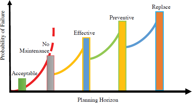
Physical and visual inspections are the most common methods of detecting cable failures. The faults determined through physical and visual inspections are generally at an advanced stage of the failure process. Inspections are generally used to detect faults in overhead cables but have limited ability to detect faults in underground cables (Gouveia 2014). Bloom and Van Reenen (2006) outlined a general decision model that enables utilities to generate business cases for asset management policies, with a specific application to underground distribution cables. The model takes a life-cycle costing approach that enables corporate financial managers and regulators to assess the multiyear financial impacts of maintaining specific classes of underground cables. Zarchi and Vahidi (2018) developed a novel algorithm for the optimal placement of underground cables in a concrete duct bank to simultaneously maximize ampacity and minimize cable system cost. Larsen (2016) described a method to estimate the costs and benefits of underground cables. The cost of moving local overhead distribution lines underground was estimated to be ∼$1 million per mile. The developed model results are most sensitive to the choice of (1) discount rates, (2) replacement cost of underground lines, (3) overhead line lifespan, (4) value of lost load, and (5) customers per line mile (Sachan and Zhou 2019). The degradation percentage in planning horizons is demonstrated in Figure 2.16. The planning stage probability of failure for cables is presented in Figure 2.17.
2.6 Smart Replacement Strategies
Monitoring strategies are crucial to extending the life of cables. Bicen (2017) presented a trend-based method to estimate the remaining service life of underground cables in which acceleration and cumulative loss of life (LOL) can be calculated continuously in small time intervals. The main novelty of this method was to determine the remaining service life of the underground cables considering the LOL trend. Electrical insulation failures occur as a result

of aging caused by the presence of stresses. It is critical to determine the stress values to define the loading conditions. Another important issue is checking the insulation and its changing conditions. In terms of insulated cables, electrical and thermal stresses are indicated as predominant aging factors. Single-stress models express lifetime as a function of only one stress prevailing over other stresses. Life models such as the inverse power law or the exponential model for electrical lifetimes, as well as other models for thermal lifetimes based on single-stress phenomena, are important for defining the replacement procedure. Zhang et al. (2021) explored advances in research and development toward cables, including smart strategies for cable inspection, condition checking and determination, fault location strategies, and cable life appraisal strategies. In their research, power flow, the change of traction power cables, and network voltage were analyzed when trains were working in traction and regenerative braking conditions.
Griffiths et al. (2002) provided a quick estimation method for the life expectancy of cables. The purpose of the paper was to introduce the extrusion process. In this process, the extrusion equipment consists of an electrically heated barrel containing a specially designed screw. In a pelletized form, the polymer is fed into the hopper at the rear of the extruder. As the polymer passes along the screw, it is melted and mixed to a homogeneous state. At the end of the barrel are mounted a head and die, through which the melted polymer passes. Cables are manufactured in conditions that exclude moisture. Therefore, precautions must be taken during installation to ensure that moisture is not permitted to enter the cable. The installation design is also outlined in this research. Essential parameters that influence smart replacement strategies are as follows:
- Depth of burial,
- Proximity of other cables,
- Temperature,
- Cable support,
- Bending radius,
- Pulling tension,
- Installation procedure,
- Duct size,
- Ground thermal resistivity, and
- Moisture (Griffiths et al. 2002).
Sachan et al. (2016) proposed a stochastic dynamic programming-based model for cable replacement optimization that takes into consideration the long-term cost of cables knowing the failure distribution and degradation of the cables. This model defines the optimum time for both maintenance and replacement. The model gives the sequence of decisions for each year of
the planning horizon. It optimizes the overall cost and improves reliability by lowering the frequency of unplanned outages. The model was tested on an unjacketed cross-linked polyethylene (XLPE) cable.
2.7 Installation Concerns
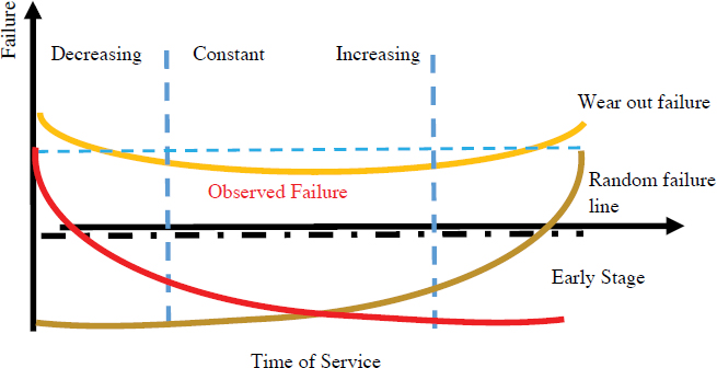
Cable failure, particularly of underground cables, is a rising concern among utilities. Underground cables are harder to access and replace because their installation cost is 10 times higher than that of overhead lines. As Figure 2.18 shows, the higher failure rates in a cable’s life cycle occur as premature failures or aging failures. The curve in the figure is known as a “bathtub curve” because of its shape. Early or premature failures are mostly because of bad installation or cable defects from manufacturing or transport. Aging results from cable operation and exposure to aging mechanisms. Generally, premature failures are not considered because it is assumed that this part of the cable lifetime occurs in the manufacture’s lab or that the defects will be detected during installation and testing procedures. The degradation level and planning horizon of cable populations installed is shown in Figure 2.18 (Sachan and Zhou 2019; Gouveia 2014).
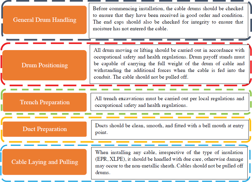
Successful transition of new cable is highly dependent on the quality of the cable and installation practices. Preventive maintenance (see Figure 2.19) is important for longer service life. Manufacturers conduct quality tests on each cable section to detect the expected fault. Transportation of cable to the site and installation activities can cause damage to the cable (Dong et al. 2017). Figure 2.20 outlines the steps (e.g., general drum handling, drum positioning, and trench preparation) in the installation process.

2.8 Cable Failure Process
Failures of cable systems are disruptive, expensive, and hazardous, and can result in loss of vital evidence. Cables, joints, terminations, and connectors that are properly installed and have not been subjected to mechanical forces, moisture, or extreme temperatures have a predictable, long service lifetime.
Cable life is mainly determined by the aging of the cable insulation. Cables can fail from any combination of electrical, mechanical, and thermal factors. Reasons for aging are shown in Figure 2.21 and can be accelerated in MV cables (Densley 2001). In Figure 2.22, conditions for cable failure are detailed. Cables fail faster when any of these four conditions occur because cable aging accelerates. Table 2.2 summarizes aging factors. These aging factors are categorized as thermal, mechanical, electrical, and environmental factors. These factors determine the mechanism and effects of aging. DC transit power cables are based on the DC nominal voltage.
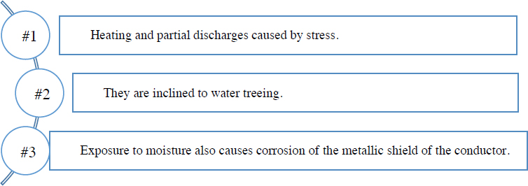

Table 2.2. Aging factors.
| Category | Aging Factor | Aging Mechanism | Effects |
|---|---|---|---|
| Thermal | High-temperature cycling Low temperature | Chemical reaction | Hardening, softening, loss of mechanical strength, embrittlement |
| Incompatibility of materials | Rotation of cable | ||
| Thermal expansion | Shrinkage, loss of adhesion, separation, delamination at interfaces | ||
| Diffusion | Increased migration of components | ||
| Annual locked-in mechanical stresses | Loss of liquids, gases | ||
| Melting/flow of insulation | Penetration | ||
| Cracking | Shrinkage, loss of adhesion, separation, delamination at interfaces | ||
| Thermal contraction | Loss/ingress of liquid | ||
| Movement of joints, terminations | |||
| Mechanical | Tensile, compressive, shear stresses, fatigue, cyclic bending, vibration | Yielding of materials | Mechanical rupture |
| Cracking | Loss of adhesion, separation, delamination at interfaces | ||
| Rupture | Loss/ingress of liquids, gases | ||
| Electrical | Voltage, AC, DC, impulse current | Partial discharges | Erosion of insulation |
| Electrical treeing | Partial discharges | ||
| Water treeing | Increased losses | ||
| Dielectric losses and capacitance | Increased temperature, thermal aging, thermal runaway | ||
| Overheating | Increased temperature, thermal aging, thermal runaway | ||
| Environmental | Water/humidity, liquids/gases, contamination | Dielectric losses and capacitance | Increased temperature, thermal aging, thermal runaway |
| Electrical tracking | Increased losses | ||
| Water treeing | Flashover |
Source: Densley 2001.

Cable with 2 kV AC insulation level and below can be single-conductor unshielded cable. All cables above 2 kV and classified as MV are shielded. DC cables can have accelerated damage, as shown in Figure 2.23.
As illustrated in Figure 2.21 and Table 2.2, aging and deterioration result from environmental and operating conditions. The operational variations that cables are subjected to result in more rapid deterioration (Densley 2001). Manufacturers use designs that inhibit known deterioration mechanisms. The stages that a new cable or cable improvement follows are described in Figure 2.24. Improving design, material selection, or manufacturing can extend cable service life. The manufacturer determines life expectancy through aging tests that should result in either a longer time to fail or higher dielectric strength. Types of failures are given in Figure 2.25, and failures to order are given in Figure 2.26. According to Villaran and Lofaro (2009), cable conditions can be classified into various categories. Classified inspection methods are listed in Table 2.3. Table 2.4 describes cable information gathering for system definition.
2.9 Conclusions
In this chapter, answers to key questions were provided to address the problems faced by agencies. Several research findings were presented to help agencies determine the lifetime of cables and the replacement time needed to replace underground cables. Table 2.5 provides responses to important questions. Table 2.6 provides a summary of the literature review. The estimated lifetime of underground cables is around 35 to 40 years. There are various test methods available to detect failures in cables. Visual inspections are performed in manholes and taps,
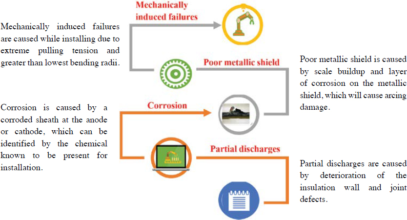
Table 2.3. Cable inspection methods.
| Visual inspection | Inspecting electrical cables by eye, on-site, to assess any physical changes. Does not require any special equipment but must be performed by experienced personnel. |
| Compressive modulus | Compressive modulus can be defined as the stress–strain ratio below a proportional limit. The aging of cable insulation and jacketing material makes the material harder and increases compressive modulus accordingly. |
| Dielectric loss | Consists of the dissipation factor test and the power factor test. The concept behind this test is that when insulation material is degraded, more leakage is present. |
| Insulation resistance and polarization index | Includes the application of a current between the cable conductor and a ground to define the insulation’s resistance between them. |
| AC voltage withstand test | A cable’s insulation is exposed to a high voltage in a very low frequency to determine whether the insulation can withstand this high voltage. |
| Partial discharge test | This test includes applying high-voltage stress through a cable’s insulation to create a partial discharge in the minor voids existing within the insulation. The occurrence of partial discharges shows the existence of degradation spots in the insulation. |
| DC high-potential test | The cable’s insulation is exposed to a high-voltage potential to determine whether the insulation can survive a potential higher than anticipated in service for a particular period. |
| Step voltage test | The cable’s insulation is exposed to a voltage that begins low and is increased in stages until the maximum test voltage is reached. |
| Time-domain reflectometry | Similar in principle to radar. A pulse of energy is conducted through a cable from one end and is reflected when it encounters either the other end of the cable or a fault in the cable. |
| Infrared (IR) thermography | A thermal detection system is used to measure the heat emitted by an object. |
| Illuminated borescope | An enhanced visual test for inaccessible areas. |
| Line resonance analysis | Uses a waveform generator and analyzes electrical test signals to detect changes in the cable insulation’s properties. |
Table 2.4. Cable information gathering for system definition.
| DC transit system nominal rated voltage | 500 V, 750 V, 1,000 V, 1,500 V, and 2,000 V are the most common. This is important information for selection of the DC cable insulation level. The cable can be 2 kV AC unshielded for systems up to 750 V DC. For 1,000 V and 1,500 V DC, it may be 5 kV shielded single-conductor cable. But the shield has no place to ground, unlike AC power supply shielded cables. |
| DC cable rated voltage | 2 kV unshielded or 5 kV single-conductor shielded MV cable. This is very important information for cables. |
| DC cable shield | It is important to consider DC cable damage at cable termination with the shield, which may allow moisture that damages the cable. |
| DC surge arrester application | Applied at traction power substations’ disconnect switches located outside the DC switchgear for third-rail power supplies, or on the feeder poles for overhead contact system (OCS) power supply or DC disconnect switches along the tracks at cross-over locations. |
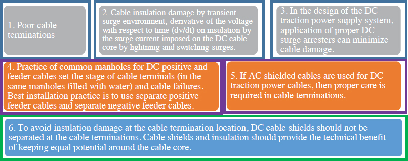
| DC cable distribution system | Common or separate manholes are used for positive and negative DC feeder cables in the distribution system. If common manholes are used for positive feeders and negative feeders, then there should be a barrier in the manholes, and care should be taken that water cannot go from one partition to the other, causing cable termination damage to positive and negative feeder cables or faults between positive and negative feeders, which can lead to an explosion hazard. |
| Surge environment at transit site | In higher lightning areas, a DC transit system will be exposed to lightning, causing direct and indirect lightning surge propagating over the DC power system, including DC cables. In addition, internal switching surges from OCS contact wire arcs and third-rail DC power supply by shoe contact subject to arcing can induce transient over-voltages. These transient over-voltages superimposed on a DC cable system can cause cable insulation weakening over time unless proper DC surge arresters are used. IEEE Std. 1627 (2019) is used to mitigate surge energy safely to ground. |
| DC voltage regulation | DC voltage is regulated at the transit facility by online voltage monitors. Such voltage regulation is required for design application of properly rated DC surge arresters to prevent DC cable insulation damage. |
Table 2.5. Responses to important questions.
|
DC transit cables are installed between traction power substations (TPSSs) and the positive power supply feed point. A TPSS is an electrical enclosure with a DC switchgear and a negative bus box. Positive feeder cable installation routing is from the DC breakers (located inside the DC switchgear) by overhead or underground polyvinyl chloride (PVC) conduits to the positive supply feed point. In case of third rail, routing is from the cable connection point to the third rail, which is the positive power supply rail (mounted on insulators parallel to the running rails). In the case of an OCS system, the routing is from the connection point to the overhead contact wire supported by messenger wire to double-insulated supports to the hollow feeder poles. Positive feeder cables are pulled either underground or aboveground using PVC conduits from the DC switchgear. The maximum length of these cables without cable splices should be 1,500 ft. Some industry practice is to install these cables without splices between the DC switchgear and the supply point location. Conduit sizes vary from 4 in., 5 in., and 6 in., depending on the size of the cables [500 MCM (thousands of circular mils), 750 MCM, 1,000 MCM] and number of cables installed in each conduit. A DC sectionalizing scheme is used for the third-rail and the OCS power supply system to determine the parallel sets of cables (generally four for a simple sectionalizing scheme for a double-track rail transit system). The number of DC feeder cables is determined by the traction power load and ampacity of each feeder cable. The number of cables should be based on maximum cable loading, not to exceed 80% of the cable rating, to allow for cables to not overheat during peak-hour operation and to accommodate some future load growth. Voltage loss in cables should be minimized for energy efficiency. Thus, the DC power supply voltage should be kept as close to the rated voltage as possible. Higher supplied voltage to the cable will lower losses but will cause higher stress on the cable. This should be considered to have optimized balance of the cable voltage and cable supply current. To keep lower voltage losses, it is good practice to install a greater number of parallel feeder cables inside the conduits. No conduit should be filled more than 40% its area. Properly rated metal oxide varistor (MOV) DC surge arresters should be installed at cable termination locations on the third rail at OCS feeder poles with disconnect switches. At wayside DC disconnect switches, MOV surge arresters keep DC feeder cables protected from transit over-voltage surges that can compromise and degrade the cable insulation level. |
|
Visual signs exist at cable termination points, DC switchgears, or positive third-rail termination locations. Another visual sign is water in the cable cracks. Inspection of cables should be routine. There should be spare conduits in place, so that if cable replacement is considered essential, it can be done without system shutdown or with minimum down time. Conditions for maximum useful life: (a) No cable insulation damage when cables are pulled through conduits, manholes, or pull boxes; (b) no major changes in loads; (c) no major overloading of cables; (d) voltage regulation is kept steady; (e) transit over-voltage is illuminated by use of proper surge limiters; and (f) cables are tested and inspected regularly. |
Table 2.6. A summary of the literature review.
| Useful Life of Cables | |
|---|---|
| Publication | Description/Relevant Points |
| Zhou et al. (2017) | The percentage of joint failures, termination failures, and cable body failures was 37%, 32%, and 31%, respectively. |
| Levi and Shah (2018) | Discusses typical construction of a medium-voltage cable. |
| Aldhuwaian (2015); Reid et al. (2013) | Contains an underground insulation material chart. |
| Altamirano et al. (2010); Densley (2001) | Cable aging, mechanisms, and consequences. |
| Terezia (2013) | The growth of water trees in insulation systems plays an important role in cable degradation. |
| Mashikian and Szarkowski (2006) | Water treeing will not inherently cause a fault in the cable. A water tree could even bore through the whole insulation and not cause a fault. |
| Lanz and Chatterton (2018); Dodds (2017) | Electrical trees in the insulation are usually visible to the naked eye. |
| Laurent et al. (2013) | If a water tree is present, it can hinder the growth of the electrical tree. Another factor is the voltage level when the electrical tree starts to discharge. |
| Lanz and Chatterton (2018) | Overheating can affect underground cable systems. |
| Lanz and Chatterton (2018) | Installation errors are one of the most common yet most preventable agents of cable faults. |
| Degree of Degradation | |
| Publication | Description/Relevant Points |
| Chang et al. (2018) | Give a predictive model of the degradation of cable insulation subject to radiation and temperature. |
| Chou and Liu (2013) | The virtual degradation rate is determined by fitting experimental data with physics-based equations. |
| Neier et al. (2019) | A method of degradation measurement is described that uses permittivity of polymers and the dielectric and mechanical measurements of aged wire insulation. |
| Szatmári et al. (2015) | The degradation process starts with bio-deterioration of the outer polyethylene layer, which can be prevented to some extent by cathodic protection. |
| Detect Degradation of Cables | |
| Publication | Description/Relevant Points |
| Meijer et al. (2015) | A health monitoring index tool was introduced to assess a cable system’s health and to evaluate maintenance strategies. |
| Sidhu and Xu (2010) | Proposed a scheme for early detection of underground cable faults. |
| Sachan et al. (2016) | Developed a probabilistic dynamic programming model to find the optimal maintenance policy for cables using the degradation level and failure distribution of cables. |
| Orille-Fernández et al. (2006) | Used artificial intelligence (ANNs) to predict the cable’s failure risk. |
| Kauhaniemi et al. (2019) | Proposed that the wave propagation velocity of the cable could be determined experimentally to enable locating of PD faults with increasing accuracy. |
| Zhang et al. (2021) | Proposed a strategy of utilizing infrared temperature estimation to accurately decide the type and degree of cable defect. |
| Ocuon et al. (2015) | Presents a thermal examination with FEM for underground cable systems. Applies momentum-type particle swarm optimization. |
| Kruizinga (2017) | The replacement of grid sections only takes place after repeated outages in the same section, as there are no methods available to perform diagnosis on LV grids. |
| Nemati et al. (2019) | The effects of control cables’ reparability characteristics on failure rate estimation are shown. |
| Factors Influencing the Lifespan | |
| Publication | Description/Relevant Points |
| Sutton et al. (2010) | Various environmental factors influence the lifespan of cables. |
| Kim et al. (2014) | Economic feasibility evaluation and simulation study results helped determine the appropriate type of cables. |
| Jones and McManus (2010) | Define the life-cycle effects of five different types of electrical cables. |
| Gouda et al. (2009) | Studied the dry-zone phenomena linked to various parameters affecting underground cables. |
| Neier et al. (2019) | After weak spots are cleared, the general aging condition of the cable can be judged, and the remaining lifetime can be estimated. |
| Ildstad (2004) | Explored factors influencing the lifespan of cables. |
| Aizpurua et al. (2021) | Developed a novel cable lifetime estimation framework that connects data-driven probabilistic uncertainty models with physics-of-failure–based operation. |
| Neier et al. (2019) | Studied an approach to estimating underground cables’ remaining life that depends on defining the weak points. |
| Zawaira et al. (2017) | Provides a power transmission line model that combines wavelets and the neuro-fuzzy technique for fault location and identification in underground cables. |
| Metwally (2011) | Discussed some preventive maintenance techniques for cables. |
| Cost-Effective Methods to Extend the Lifespan | |
| Publication | Description/Relevant Points |
| Gouveia (2014) | Inspections are generally used to detect faults in overhead cables but have limited ability to detect faults in underground cables. |
| Bloom and Van Reenen (2006) | A decision model is presented that enables utilities to generate business cases for asset management policies. |
| Zarchi and Vahidi (2018) | Contains a novel algorithm for the optimal placement of underground cables in concrete duct banks to simultaneously maximize ampacity and minimize cable system cost. |
| Larsen (2016) | Presents a method to estimate the costs and benefits of underground cables. |
| Sachan and Zhou (2019) | A degradation percentage in planning horizons is demonstrated. |
| Smart Replacement Strategy | |
| Publication | Description/Relevant Points |
| Bicen (2017) | Presents a trend-based method to estimate the remaining service life of underground cables. |
| Zhang et al. (2021) | Explore latest advances in research and development toward cables, including smart strategies for cable inspection. |
| Griffiths et al. (2002) | Provide a method for quick estimation of the life expectancy of cables. |
| Sachan et al. (2016) | Provides a stochastic dynamic programming-based model for cables replacement optimization. |
| Installation Concerns | |
| Publication | Description/Relevant Points |
| Sachan and Zhou (2019) | Cable degradation can be quantified in terms of percentage of life remaining with the advancement of age for a group of cables with similar installation years, design, and operation. |
| Dong et al. (2017) | Transportation of cables to the site and installation activities can cause damage. |
| Cable Failures Process | |
| Publication | Description/Relevant Points |
| Densley (2001) | Represented reasons for aging degradation, which can be accelerated in medium-voltage cables. Aging and deterioration result from environmental conditions. |
| Villaran and Lofaro (2009) | Represented cable conditions inspection methods. |
and hi-pot, meggering, and thumb tests are run at certain periods to determine and fix cable faults. In addition, the Blavier test can be performed when there is a ground fault in one cable and there are no other faulted cables. The Blavier test is the measurement of resistance from the end of one segment. This test is considered a cost-effective method that can be used to identify cables that may need replacement. Although the tests are relatively straightforward, repair or replacement can be challenging and complex work, and more equipment may be needed to detect faults in traction cables. Fast and effective cable failure detection is critical and reduces the possibility of higher risks. The key features for installing underground cables are the distance between the cables, insulation size, depth of burial, ground thermal resistivity, temperature, and the cable support system. This chapter has reviewed the parameters to be used during the installation of underground cables. In addition, the parameters that are required to test underground cable resistivity due to aging have been summarized. New insulation materials have provided a new aspect to cable service life. In addition, condition assessment and failure prediction are important for longer cable service life. Even the failure mechanisms are different in various cases, and as such cable monitoring is very important. Currently, there is a lack of knowledge regarding condition assessment data in the existing models. It is also important to carry out research to improve condition assessment of a cable’s actual condition and remaining life. Artificial intelligence techniques can be helpful in this regard. To determine the failure modes in cables, models for degradation are used to determine the level of degradation in cables. The keys to improved assessment of cable integrity and life expectancy are the identification of degradation and determining its rate of progress to obtain an accurate prediction of failure. Various health monitoring systems
have been developed, and data from these systems are used in the assessment and prediction of degradation in cables and can help determine remaining cable lifetime.
Various techniques can be used to identify failure causes, and these techniques may help improve cable design, manufacturing processes, decision-making processes, installation practices, and condition assessment. For prediction of age-related failures, statistical approaches can be used. Detailed analysis of the causes of early failures and failure rate prediction can be done using a combination of multiple approaches. For instance, a combination of physics-based multi-model analysis, statistical analysis, and artificial intelligence provides the most meaningful and accurate assessment and predicting approach. For precise modeling of condition assessment, all parameters should be considered. Most methods used to predict cable failures have been based on historical failure data. The key parameters are the impact of electrical surges, water ingress, mechanical damage, imperfections in manufacturing, and improper installation processes. These parameters should also be considered in the cable service life and failure prediction models. In the cable failure prediction models, there is a need for development of the aging and failure relationship. In addition, the effects of local climate and water on the degradation process of cables need to be considered when assessing regional variations in cable life expectancy.


