Page 110

Suggested Citation: "5 Cable Replacement." National Academies of Sciences, Engineering, and Medicine. 2024. Transit Traction Power Cables: Replacement Guidelines. Washington, DC: The National Academies Press. doi: 10.17226/27907.

CHAPTER 5 Cable Replacement

Cable replacement is investigated in this chapter. First, an optimization model is provided for the traction power cables. Then, finite element analysis is carried out for cables. These two actions are connected since load factor plays an important role in determining cable service life.

In Figure 5.1, a flowchart is provided that presents an estimation method for determining cable lifetime. A realistic estimation is based on a realistic model and analysis. In this chapter, a life model was created for accurate estimation. In Section 5.1, a cable degradation model is provided as a part of the optimization process. In Section 5.2, an optimization model was presented for cable maintenance and replacement. In Section 5.3, a cable failure rate model for estimation is presented. An optimal replacement period is calculated in Section 5.4. In Section 5.5, the optimal cable replacement period is discussed. Finite element analysis is provided in Section 5.6.

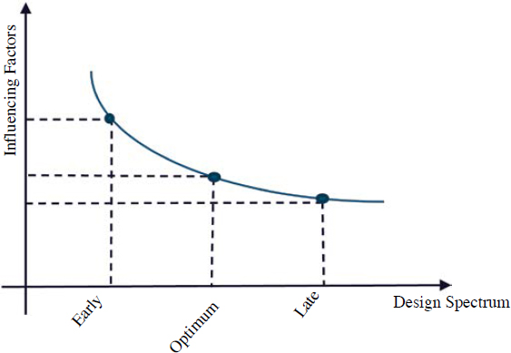
As part of the optimization process, load factor, environmental characteristics, and installation conditions are considered in the model. These factors are dynamic and can reduce or increase the expected lifetime. Figure 5.2 presents the design spectrum curve considering influencing factors. Model development with dynamic factors is based on this curve. The model presents an optimum period in the design spectrum curve. Cable lifetime is related to the dynamic factors and should be monitored for determining the remaining cable lifetime. Even though this curve is important, it is not the only approach to determining the lifetime. There are various parameters affecting the lifetime calculation process.

5.1 Cable Degradation Estimation for the Optimization Model

In this section, a model is introduced for determining the degree of cable degradation based on the actions taken at each decision epoch. Considering that cables are tested annually and that proactive and reactive maintenance and replacement decisions are made based on the test results, it is assumed that the time between two consecutive epochs is 1 year. The degradation estimation model created in the research was used to estimate the future degradation values over the planning horizon, which may be up to 100 years.

Figure 5.3 depicts the degradation process used in the research. At each decision epoch, an alternative from among maintenance interventions, cable replacement, and doing nothing was selected. Note that the “do nothing” option was kept until the following decision epoch in the proposed set. For simplification, two maintenance interventions were included, whereas the actual number of interventions can be different for each transit agency. The proposed model readily extends to any number of maintenance interventions.

In Figure 5.3, the current epoch is represented by t, where the current degree of degradation is observed. Assume that d_t is the degree of degradation of insulated cables at the beginning of the

Page 111

Suggested Citation: "5 Cable Replacement." National Academies of Sciences, Engineering, and Medicine. 2024. Transit Traction Power Cables: Replacement Guidelines. Washington, DC: The National Academies Press. doi: 10.17226/27907.

Installation Conditions

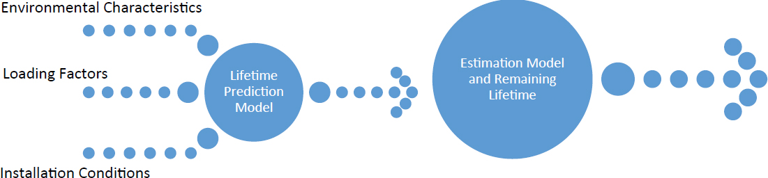
***Figure 5.1. Flowchart presenting estimation method.***

***Figure 5.2. Design spectrum curve.***

***Figure 5.3. Degradation model for the optimization process.***

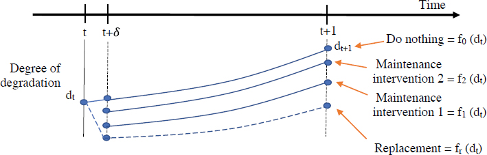
decision epoch t. This could be estimated based on the annual test results and visual inspection. At this point, the optimization model decides on the best decision alternative among doing nothing, replacement, and maintenance interventions 1 and 2. Upon the given decision, the degree of the degradation is updated (i.e., degradation is reduced via maintenance interventions and degradation is eliminated after replacement, as shown at t + δ). Time after the intervention (maintenance or replacement) δ is assumed to be small. For the continuity and consistency of the model, degree of degradation was determined at the beginning of the next decision epoch (t + 1) based on the decision made at t. Let f₀(d_t), f₁(d_t), f₂(d_t), and f_r(d_t) represent the degree of degradation at the beginning of next decision epoch (t + 1) respectively for doing nothing, maintenance intervention 1, maintenance intervention 2, and cable replacement, where the current degradation before the intervention at t is measured as d_t. The estimation of these functions is critical for the validity of the model.

Page 112

Suggested Citation: "5 Cable Replacement." National Academies of Sciences, Engineering, and Medicine. 2024. Transit Traction Power Cables: Replacement Guidelines. Washington, DC: The National Academies Press. doi: 10.17226/27907.

5.2 Optimization Model for Cable Maintenance and Replacement

The proposed optimal maintenance and replacement schedule problem identifies the best intervention to minimize the average maintenance and replacement cost over the planning horizon T while sustaining a safe and reliable system. At each decision epoch t ∈ {1, … , T}, the model identifies the best alternative among doing nothing, maintenance interventions 1 and 2, and cable replacement. This model introduces the binary variables to represent the intervention alternatives.

$x_{0 t} = {\begin{array}{l} 1 & if “ do nothing ” alternative is selected at decisione poch t \\ 0 & otherwise \end{array}$

$x_{1 t} = {\begin{array}{l} 1 & if maintenance intervention 1 is selected at decision epoch t \\ 0 & otherwise \end{array}$

$x_{2 t} = {\begin{array}{l} 1 & if maintenance intervention 2 is selected at decision epoch t \\ 0 & otherwise \end{array}$

$x_{x t} = {\begin{array}{l} 1 & if cable replacement is selected at decision epoch t \\ 0 & otherwise \end{array}$

Next, to formulate the optimization model, the following was established:

$Minimize \sum_{t = 1}^{T} c_{1} x_{1 t} + c_{2} x_{2 t} + c_{r} x_{r t}$

(5.1)

subject to

$d_{t + 1} = f_{0 t} (d_{t}) x_{0 t} + f_{1 t} (d_{t}) x_{1 t} + f_{2 t} (d_{t}) x_{2 t} + f_{r t} (d_{t}) x_{r t}, \forall t \in {1, \dots, T}$

(5.2)

$x_{0 t} + x_{1 t} + x_{2 t} + x_{r t} = 1 \forall t \in {1, \dots, T}$

(5.3)

$d_{t} \leq d_{max}, \forall t \in {2, 3, \dots, T + 1}$

(5.4)

$x_{0 t}, x_{1 t}, x_{2 t}, x_{r t} \in {0, 1}, \forall t \in {0, \dots, 1}$

(5.5)

The objective function formulated in Equation 5.1 minimizes the cost of maintenance and replacement over the planning horizon, where a linear cost function is adopted with c₁ and c₂ respectively represent cost of maintenance interventions 1 and 2, and c_r is the cost of cable replacement. It is assumed that the cost parameters do not change with time and are not affected by the degree of degradation at the time of the intervention. Since the survey results show that the cost of maintenance interventions depends on the degree of degradation of the cables, the objective function formulation can be revised as follows in Equation 5.6:

$\sum_{t = 1}^{T} c_{1} (d_{t}) x_{1 t} + c_{2} (d_{t}) x_{2 t} + c_{r} x_{r t}$

(5.6)

Where the functions c₁ (d_t) and c₂ (d_t) represent cost of maintenance interventions 1 and 2, when the degree of degradation is d_t.

Page 113

Suggested Citation: "5 Cable Replacement." National Academies of Sciences, Engineering, and Medicine. 2024. Transit Traction Power Cables: Replacement Guidelines. Washington, DC: The National Academies Press. doi: 10.17226/27907.

Constraints in Equation 5.2 determine the degree of degradation at the next decision epoch, d_(t+1), given the selected intervention and initial degree of degradation d_t. Constraints in Equation 5.3 impose that only one intervention alternative can be selected at each decision epoch, where doing nothing is counted as an intervention for simplicity. If multiple interventions are needed simultaneously, the constraints in Equation 5.3 can be revised accordingly. The constraints in Equation 5.4 enforce that the degree of degradation at any decision epoch be less than or equal to a predetermined maximum degradation threshold, d_max. Solving the problem with different thresholds, a trade-off curve between cost and reliability can be obtained. End users may select the best alternative for their priorities. Finally, the constraints in Equation 5.5 were the binary restrictions on the decision variables representing the interventions.

5.3 Cable Failure Rate Estimation

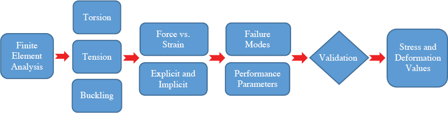
The failure rate models can be estimated using historical failure records. Currently, there is no database available containing failure records for transit power cables. The FTA or another agency or association could initiate the development of a secure online database where transit agencies can report power cable failures. Each failure record could include insulation type, jacket type, conduit, rated voltage, cable age, presence of water, exposure to extreme temperatures, whether underground or overhead, length of the power cable segment, the number of previous repairs on the cable, and maintenance period. Many of these factors were mentioned by the respondents to this project’s survey. Survey participants mentioned water and temperature as environmental parameters affecting the useful life of transit power cables. Furthermore, many participants listed jacketing and conduits as the most important physical parameters of cable design that affect the life of transit power cables. Thus, these factors are included as potential model parameters to estimate the cable failure rate. Additionally, the length of the cable segment has been added to normalize failure rates. In the literature, insulation and rated voltage have been used extensively in cable failure rate models. The age of the failed cable segment is also needed for the failure models. Figure 5.4 illustrates the performance determination process for cables.

If the locations of the previous failures are recorded, possible failure locations can be defined with a historical pattern. The data structures that are suggested to be used for cable capital, past failures, and testing and preventive maintenance data collection are listed in Tables 5.1, 5.2, and 5.3, respectively. These tables are used in the performance determination process and are therefore important to the proposed procedure.

***Figure 5.4. Cable performance determination process.***

Page 114

Suggested Citation: "5 Cable Replacement." National Academies of Sciences, Engineering, and Medicine. 2024. Transit Traction Power Cables: Replacement Guidelines. Washington, DC: The National Academies Press. doi: 10.17226/27907.

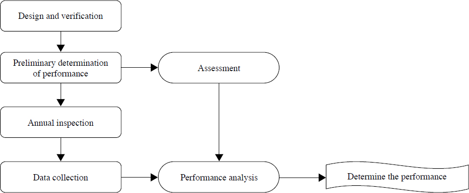
Table 5.1. Cable capital data collection.

Cable Capital
Location Installation year Cable function Length Conduit Insulation type Jacketing Low smoke zero halogen	Presence of water Exposure to extreme temperatures Underground/overhead Testing frequency (per year) Test type Last test date Last test result Scheduled test date

Table 5.2. Historical failure data collection.

Historical Failure Data
Cable ID Location Date of failure Emergency status Failure mode Aggravating factors Date of repair The number of previous repairs	Time to repair the cable Cost of materials Cost of labor System downtime cost Other costs Replace or repair

Table 5.3. Testing and preventive maintenance data collection.

Testing and Preventive Maintenance Data
Cable ID Test date Test type Test result Cable state classification (excellent, good, fair, needs replacement) Cost of test	Cable ID Preventive maintenance date Preventive maintenance type Cost of preventive maintenance

Some challenges can be expected in the proposed procedure. These challenges are related to the nature of the problem, and some solutions can be proposed to overcome them. First, if the installation date of a cable is not known, the purchase date of the cable can be used as a reasonable approximation of the installation date. Additionally, manufactured date and other related data are printed on the cable jacket. These data should be readable for the maintenance, repair, and replacement processes.

Second, the number of failures in the created database may not be sufficient to build robust statistical models that consider the number of levels of model factors, especially age of the cable. Ineffective factors can be identified and removed from the model to make it more meaningful. Furthermore, bins can be used to represent the age of the failed cables. For instance, 5-year or 10-year bins may generate enough data points in the process for a strong statistical model.

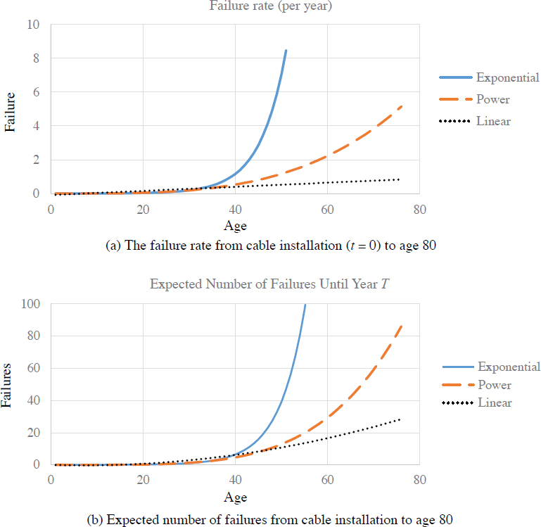
The failure rate of cables can be modeled as exponential, power, and linear functions of time [i.e., λ^E(t) = ae^bt, λ^P(t) = at^b, and λ^L(t) = a + bt]. Using historical cable failure data, these three models can be tested using a goodness-of-fit test. As new failure data become available, the statistical models can be updated. A failure rate function, λ_i(t), is estimated for each factor combination i. Let λ(t) be the vector of failure rates for each factor combination. The expected number of failures is calculated based on the time of the cable installation to t = T. A non-homogeneous Poisson process was carried out as the underlying failure model, as seen widely in the literature. Let Λ_i(T) be the number of expected failures: Λ_i(T) = ∫^T_t₌₀λ_i(t)d_t. Hence, the

Page 115

Suggested Citation: "5 Cable Replacement." National Academies of Sciences, Engineering, and Medicine. 2024. Transit Traction Power Cables: Replacement Guidelines. Washington, DC: The National Academies Press. doi: 10.17226/27907.

expected number of failures with failure rate models using three different function models as exponential, power, and linear functions is determined as given in Equation 5.7.

$Λ^{E} (T) = \frac{a}{b} (e^{b T - 1}) for exponential$

$Λ^{E} (T) = \frac{a}{b + 1} T^{b + 1} for power$

$Λ^{E} (T) = a T \frac{b}{2} T^{2} for linear$

(5.7)

At this point, the cables with the highest failure rates can be identified. These cables can be given priority in the replacement schedule. The preliminary analysis can also reveal the factors that significantly affect cable failures. The cable or design with a low failure rate and high reliability can be identified. The methodology is summarized in Table 5.4, whereas Tables 5.5, 5.6, and 5.7 provide information about predictive analytics, testing schedules, and cable replacement. In this procedure, creating and managing a sufficient database is not an easy task. Therefore, this step would be the most challenging part of the procedure and could be critical for the success of the model.

Table 5.4. Data analysis plan.

Data collection for descriptive analytics	Cable capital Historical failure data Testing and preventive maintenance data
Predictive analytics	Estimate cable test results Estimate failure rates
Prescriptive analytics	Testing, preventive maintenance, replacement schedules

Table 5.5. Predictive analytics.

Estimate Cable Test Results	Estimate Cable Failure Rates
Test type Cable age Jacket type Insulation type Conduit Previous test results	Exponential, power, linear functions Cable age Jacket type Insulation type Conduit type

Table 5.6. Testing schedules.

Inputs	Output
Cable capital Time required for testing Number of technicians Other assignment restrictions (e.g., time of the day for testing)	Test schedule for technicians, where, All cables are tested and The workload is fairly distributed among technicians and throughout the year.

Table 5.7. Cable replacement.

Inputs	Output
Estimated cable failure rate function Cost of failure Cost of replacement	The optimal time to replace the cable

Page 116

Suggested Citation: "5 Cable Replacement." National Academies of Sciences, Engineering, and Medicine. 2024. Transit Traction Power Cables: Replacement Guidelines. Washington, DC: The National Academies Press. doi: 10.17226/27907.

Table 5.8. Data challenges.

Data Challenges
Estimating cable failure rate	Data are not available. Failures are rare events. Data accumulation is very slow.
Estimating cost of failure	Significant variation in the cost-of-service interruption, cost of losing customer goodwill.
Estimating cost of replacement	Many variables affect the cable cost (e.g., jacketing, insulation, conduit). Effect of economies of scale (replacing multiple cables).

Table 5.8 summarizes some of the expected data challenges. As mentioned, in modeling some data, challenging issues are expected; these are listed in this table. Cable capital and historical failure data samples are presented in Tables 5.9 and 5.10.

The failure rate behaviors and expected number of failures are presented from the cable installation to year T based on a large U.S. underground distribution system dataset from the literature (Zhou and Brown 2006). Note that the failure rate models must be constructed using failure records from U.S. transit agencies. For this analysis, it is assumed that the length of the cable is 5 miles. Figure 5.5.a shows the failure rate from cable installation (t = 0) to age 80, whereas Figure 5.5.b displays the expected number of failures from cable installation to age 80, using the exponential, power, and linear functions to model failure rate behavior. Using the power function for modeling the failure rate, Figure 5.5.a shows that the failure rate is around two when the cable age is 60 (i.e., two failures per year on this 5-mile transit traction power cable). Using the same failure model, Figure 5.5.b shows that the expected number of failures from installation to year 60 is around 30.

Table 5.9. Cable capital sample.

Location	Insulation Type	Jacket Type	Conduit	Rated Voltage	Cable Age	Length of the Cable Segment	Presence of Water	Corrosion	Exposure to Extreme Temperatures	Underground/Overhead	Maintenance Frequency per Year
Banfield	EPR	XLPE	Yes	2 kV	1987	400 ft	Moderate	Low	Low	UG	1.0
Fuller	EPR	XLPE	Yes	2 kV	2009	1,000 ft	High	Low	Low	UG	1.0
Lincoln	EPR	XLPE	Yes	2 kV	2009	350 ft	Low	Low	Low	UG	1.0
East Portal	EPR	XLPE	Yes	2 kV	1998	250/3,150 ft	Moderate	Low	Low	UG/UF	1.0
Bybee	EPR	XLPE	Yes	2 kV	2015	600 ft	High	Low	Low	UG	1.0
Sunset	EPR	XLPE	Yes	2 kV	1998	400 ft	Low	Low	Low	UG	1.0
Mt. Hood	EPR	XLPE	Yes	2 kV	2001	400 ft	High	Low	Low	UG	1.0
Steel Br.	EPR	XLPE	Yes	2 kV	1986	1,000/1,850 ft	Moderate	Moderate	Low	UG/UF	1.0
Parkrose	EPR	XLPE	Yes	2 kV	2001	850 ft	Low	Low	Low	UG	1.0
Gateway	EPR	XLPE	Yes	2 kV	1998	1,000 ft	Low	Moderate	Low	UG	1.0

Notes: UG = underground; UF = underground feeder.

Page 117

Suggested Citation: "5 Cable Replacement." National Academies of Sciences, Engineering, and Medicine. 2024. Transit Traction Power Cables: Replacement Guidelines. Washington, DC: The National Academies Press. doi: 10.17226/27907.

Table 5.10. Historical failure data sample.

Failure #	Location	Date of Failure	Cost of Repair/Replacement	Downtime Cost	The Number of Previous Repairs for the Location	Failure Mode (if known)	Aggravating Factors
1	5th Market	7/11/2014	$15,000	$0	None	Corrosion	Bad Tap
2	32nd	2/6/16	$9,086	$0	None	Corrosion	Bad installation
3	East Portal	11/2016	$9,125	Yes	None	Insulation failure	Damage on installation
4	Hillsboro	4/25/2018	$8,280	Yes	None	Insulation failure	Damage on installation
5	6th Mad	3/12/2019	$18,169	Yes	None	Insulation failure	Damage on installation

***Figure 5.5. Estimation of failures from cable installation.***

Page 118

Suggested Citation: "5 Cable Replacement." National Academies of Sciences, Engineering, and Medicine. 2024. Transit Traction Power Cables: Replacement Guidelines. Washington, DC: The National Academies Press. doi: 10.17226/27907.

5.4 Optimal Replacement Period

The primary objective of the optimal maintenance and replacement schedule is determined by the transit agency. Among the many alternatives, minimization of the average costs and maximization of the availability of the transport systems are widely used as objectives. In this report, the focus is to minimize the average cost.

Let λ_i(0) be the failure rate of a newly installed cable segment with configuration i. After t years, and possibly maintenance operations and repairs, the system operates with the failure rate λ_i(t). The new failure rate is estimated using the model developed in the previous section (see Figure 5.5.a).

The objective function includes the cost of maintenance, repairs, and replacement from cable installation to time t. The total cost of failure consists of the repair cost, the cost of not being able to transport passengers, and the cost of any other issues arising due to a failure in the link. While the repair cost can be estimated relatively easily, it is challenging to estimate costs of not transporting passengers and other issues. The survey participants were asked about the repair methods they used for failures and the estimated cost of repairs. All the participants answered this question saying that they have been splicing the cable for repairs. The cost and duration of the repairs depends on the size and location of the failures in the cable. The cost of a splice kit is around $500. The labor cost should be counted toward the repair cost as well. The cost of not transporting passengers depends on the number of passengers using the affected network and alternative routes that could be offered. This cost should be investigated for each link in each network for a reliable estimate. Like the repair cost, the replacement cost was estimated, which depends on the cost of cable, duration of replacement processes, cost of labor, the opportunity cost of the loss of passengers, and cost from any other inconveniences. Let C^R_i be the cost of cable replacement at link i. The average of cost during [0, T] is:

$C_{i}^{T} = \frac{C_{i}^{F} \times E [N_{i}^{T}] + C_{i}^{R}}{T}$

(5.8)

where E[N_i^T] is the expected number of failures during [0, T] and can be found using the failure rates. Figure 5.6 displays average total cost and cost of failure and replacement when cable is replaced every T years, T = 1, … , 70.

***Figure 5.6. Average total cost, average cost of failure, and average replacement cost when replacement period is T Years, T = 1, … , 70.***

Page 119

Suggested Citation: "5 Cable Replacement." National Academies of Sciences, Engineering, and Medicine. 2024. Transit Traction Power Cables: Replacement Guidelines. Washington, DC: The National Academies Press. doi: 10.17226/27907.

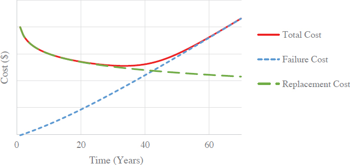
As cable ages, the failure rate increases. Then, the total cost of failures and the average cost of failures increase. On the other hand, the cost of cable replacement is fixed, C_i^R, and the average cable replacement cost decreases as the replacement period T increases. The optimal T*_i was found that minimizes the average repair and replacement cost of link i.

$Minimize \frac{C_{i}^{F} \times E [N_{i}^{T}] + C_{i}^{R}}{T}$

$s . t . T \geq 0$

(5.9)

For the cable with repair and replacement costs given in Figure 5.6, the optimal cable replacement is 33 years. Table 5.11 shows optimal replacement time (in years) based on the replacement and repair costs ratio.

If the costs of repair and replacement are not available, instead of nominal values, relative values will be sufficient for identifying the optimal replacement period. This ratio can be used to identify the optimal replacement period, which can be estimated by either analyzing historical cost values or by expert opinions.

Next, the case was investigated where multiple cables are replaced at once. This situation is expected to have significant savings in replacement cost because multiple connected cables located in the same transportation lane are replaced. For instance, transportation service is halted if one link is under construction (being replaced) or two connected links in the same transportation line are under construction (being replaced). Hence, the total replacement cost when two cables are replaced together is expected to be less than the sum of the replacement cost when two cables are replaced at different times [i.e., $C_{{i, j}}^{R} < C_{i}^{R} + C_{j}^{R}$ ].

On the other hand, cables’ individual optimal replacement periods, T_i and T_j, may be different using different approaches. These approaches can affect the optimization process. The optimal replacement period for a group of cables can be different than the optimal replacement of each cable separately. If the savings in the replacement cost of a group of cables is not significant, then it might be optimal to replace cables individually at their respective optimal replacement periods. Let T_{i,j_} be the optimal replacement period of group cables {i, j}. Then, the following are the possible cases:

$a . \frac{C_{i}^{F} \times E [N_{i}^{T}] + C_{j}^{F} \times E [N_{j}^{t}] + C_{{i, j}}^{R}}{T_{{i, j}}} < \frac{C_{i}^{F} \times E [N_{i}^{T}] + C_{i}^{R}}{T_{i}} + \frac{C_{j}^{F} \times E [N_{j}^{T}] + C_{j}^{R}}{T_{j}}$

(5.10)

$b . \frac{C_{i}^{F} \times E [N_{i}^{T}] + C_{j}^{F} \times E [N_{j}^{t}] + C_{{i, j}}^{R}}{T_{{i, j}}} \geq \frac{C_{i}^{F} \times E [N_{i}^{T}] + C_{i}^{R}}{T_{i}} + \frac{C_{j}^{F} \times E [N_{j}^{T}] + C_{j}^{R}}{T_{j}}$

(5.11)

Table 5.11. Optimal replacement time (in years) based on the ratio between failure cost and replacement cost using exponential, power, and linear failure rate functions.

	Ratio of Failure Cost to Replacement Cost
	1-to-1	1-to-10	1-to-50	1-to-100	1-to-200
Exponential	23	33	41	44	48
Power	22	36	51	58	69
Linear	15	41	80+	80+	80+

Page 120

Suggested Citation: "5 Cable Replacement." National Academies of Sciences, Engineering, and Medicine. 2024. Transit Traction Power Cables: Replacement Guidelines. Washington, DC: The National Academies Press. doi: 10.17226/27907.

***Figure 5.7. Possible inequality cases for (a) two cables or (b) a single cable.***

***Figure 5.8. Process for determining optimal cable replacement period.***

In the process, as shown in Figure 5.7, if the first inequality holds, it is cost-effective to replace the two cables simultaneously rather than replace them at different times during their respective optimal replacement periods. If the second inequality holds, then each cable should be replaced at its optimal replacement period, T_i and T_j, rather than the typical replacement period, T_{i,j}. It is important to estimate the replacement cost of a group of cables accurately at the same time. Since the number of possible groups grows exponentially, groups should be formed based on the network structure. The proximity of the links as well as the transportation lane they are located in are important factors to consider when identifying potential groups of cables to replace together.

The optimization procedure is summarized in four steps to explain the stages. This itemized four-step procedure was developed to use as an optimal cable replacement procedure. In Figure 5.8, important points in the process are depicted. The process can be carried with the data collected in the transit systems.

5.5 Process for Determining Optimal Cable Replacement Period

The four-step process for determining the optimal cable replacement period is described in the following:

For estimation of cable failure rates, all cable failures should be collected using a secure online database. Each failure record should include the following information: insulation type, jacket type, conduit, rated voltage, cable age, presence of water, exposure to extreme temperatures, whether underground or overhead, length of the power cable segment, the number of previous repairs on the cable, and maintenance period.
For each link on each network, if possible:
1. Cable repair cost should be estimated (material, labor, etc.);
2. Cable failure cost should be estimated (repair cost and cost due to loss of passengers); and
3. Cable replacement cost should be estimated (material, labor, loss of passengers, other costs).
Otherwise, the ratio between failure and replacement costs is estimated based on historical data or expert opinion.

Page 121

Suggested Citation: "5 Cable Replacement." National Academies of Sciences, Engineering, and Medicine. 2024. Transit Traction Power Cables: Replacement Guidelines. Washington, DC: The National Academies Press. doi: 10.17226/27907.

Average of optimal cost and optimal cable replacement period (T_i*) are found by calculating the average total cost for T = 1, … , 80.
Identify groups of cables (two or more) that require the closure of the same transportation lane and are in close proximity to each other. Identify the replacement cost of the group of cables and check whether cases (a) or (b) in Equations 5.10 and 5.11 hold true. Accordingly, determine whether replacing groups of cables together is cost-effective.

5.6 Finite Element Analysis

An efficient and accurate assessment of cables provides a better understanding in the evaluation process. The FEM is an efficient and accurate analysis tool for such assessment. This methodology was developed to identify the problems defined by partial differential equations. Three-dimensional analysis became possible with technology. Various software programs have been created that use the FEM. With the software, cables are modeled in layers by means of finite number of elements.

The method can be used for both linear and nonlinear analyses. The FEM involves discretization of the problem into a finite number of elements and defining equations for each element. Members are divided into meshes, and these meshes are analyzed individually. Once they are completely investigated, they are brought together to define the structural characterization of the member. The elements are assembled according to restraining factors and equations in a matrix form. The unknowns are identified by analyzing the equation sets. The finite numbers of elements are connected to each other by a finite number of meshes. The number of unknowns for each mesh is equal to its degree of freedom. The behavior of the element is defined by equations that involve these unknown degrees of freedom. The mathematical model of the structure is obtained by ensuring the continuity conditions on meshes.

In the FEM, the meshes are classified according to their geometries, such as triangle, diamond, or rectangular, number of unknowns, as well as the characteristics of the continuum problem. They can also be categorized according to mathematical modeling due to the acquisition of the basic element matrices. The accuracy of the finite element model depends on the assumption of the meshes and the number of these meshes. Generally, the number of unknowns increases parallel to the number of meshes; hence the accuracy and certainty of the results of the analyses.

There is robust literature on efficiency of the FEM in cable assessment. Labrosse et al. (2000) investigated the energy dissipated through friction due to the motions between wires when a cable is loaded. Ghoreishi et al. (2007) compared the results from linear elastic models of a single-layered strand under static axial loading. The analytical models were presented to give estimations of the elastic stiffness constants. Research carried out by Ocuon et al. (2015) presents a thermal examination of an underground power cable system. Beleznai et al. (2007) analyzed the seven-wire strand under tensile loads. Nawrocki and Labrosse (2000) presented a finite element model for simple straight-wire rope strands, which allows the study of all the possible inter-wire motions. The role of the contact conditions in pure axial loading and in axial loading combined with bending was investigated. Jiang et al. (2000) presented a concise finite element model of a three-layered straight helical wire rope strand under axial loads. For the behavior change of the wire strand, the finite element results showed better agreement with an experimental result of another study. Sathikh et al. (2000) worked with a general discrete thin-rod model to present the response of a strand of helical wires. Stanova et al. (2011) modeled wire strands to predict their behavior.

Three-dimensional (3D) geometric models of the multilayered strands and the results of the finite element elastic behavior analyses of the strand under tension loads are validated through

Page 122

Suggested Citation: "5 Cable Replacement." National Academies of Sciences, Engineering, and Medicine. 2024. Transit Traction Power Cables: Replacement Guidelines. Washington, DC: The National Academies Press. doi: 10.17226/27907.

comparisons with experimental work. Kumar and Botsis (2001) highlighted the strong influence of the material modulus of elasticity on the critical contact stresses in multilayered strands under tension and torsion.

The general finite element approach includes nonlinear and complex procedures as well. Therefore, intervention is needed for an iterative approach to be revealed. As the cables are under tension forces, a complex analysis was carried out to determine the response of the strands. The finite element method with the direct stiffness principle was taken into consideration in the modeling. Finite element analysis of the system modeled with strand elements, nodes, and supports was performed with iterative operations. Iterative operations were finalized when they reached permissible tolerance. Permissible tolerance was defined as relative differentials of the force of elements and displacements obtained from two consecutive iteration steps. Behavioral change determination was carried out under different external loads on cables. External loads were evaluated with the presented method, summarized in Figure 5.9.

Even though several operational procedures have been developed in the finite element analysis of cables, the incremental method, which considers external forces step by step, and the Newton–Raphson method, which takes forces into account that affect the static equilibrium at nodes of the deformed system, are preferred. The tangent stiffness matrix is used due to the nonlinear load–displacement relationship in both methods. The tangent stiffness matrix consists of the elastic stiffness matrix used in linear analysis and the geometrical stiffness matrix. The elastic rigidity matrix is related to elastic modulus and cross-sectional areas, while the geometric stiffness matrix is directly related to axial internal forces. Through this methodology, the tension forces at the initial steps and the internal forces in the following iteration steps can be taken into account. Tangent stiffness is reset according to the current existing geometry and internal forces of the system. While final deformations are observed, the final internal forces are determined that cause this behavioral change.

It should also be noted that the load increment value affects the sensitivity of the operation and the time-of-problem solution. The Newton–Raphson or variable stiffness method is finalized with an imbalance of forces at nodes of the deformed system according to the previous equilibrium under external loads. All external loads are applied at the same time. The initial deformations are determined from the tangent stiffness matrix obtained by the initial geometry of the undeformed system. The tangent stiffness matrix is recalculated in each step of iteration, considering the deformed cable system geometry and internal forces. As a result of the matrix solution, when the permissible tolerance is reached or if the steps do not affect the equilibrium between the external loads applied on cables and the internal forces of the system, the procedure is completed. The new position displacements are obtained for each step of the iteration. When the imbalanced forces are reached at the permissible tolerance, the procedure is finished.

As a result of the approach, if the axial force of the cable element becomes negative, it will be taken into account as zero in the next step of the procedure. So, the procedure that creates

***Figure 5.9. Finite element methodology for cables.***

Page 123

Suggested Citation: "5 Cable Replacement." National Academies of Sciences, Engineering, and Medicine. 2024. Transit Traction Power Cables: Replacement Guidelines. Washington, DC: The National Academies Press. doi: 10.17226/27907.

the part of any iteration step is completed. The material model was characterized using a linear relation between stress and strain. To define this relationship, an eight-node linear mesh element with one integration point was used in the material modeling. This element is represented in Figure 5.10. The element has three degrees of freedom per node. It was applied for the structural discretization, and wires of the strand were discretized using these elements. It has three translations for the analysis. In finite element analysis, such members are used in general purposes with a cross-sectional midpoint located in the middle of the element, as shown in Figure 5.10. The element is used mainly for tension, torsion, and bending analyses. Displacement and strain values were determined by the reference of the integration point. Since the displacement and strain values are relatively small, it was assumed that the strands stay geometrically linear.

Cables can be analyzed with the FEM via available software to determine the behavioral responses related to performance and failure. In Figure 5.11, sample cable systems that were modeled and analyzed through FEM and stress versus loading distribution are shown. As demonstrated in Figure 5.11, cables can be modeled through the FEM, and stress distribution can be defined with loading and time as well. Cables can be classified with their performance over the years, and all different parameters, such as environment, loading, location, and their life evaluation, can be based on such accurate analyses. As a part of the finite element analysis, cable models were established and analyzed.

Finite element analysis results for these models were compared for various cases. In the finite element modeling, cable material and insulation layers, cable weight, attachment points as boundary conditions, and factors such as vibrations, tension, and temperature range were considered and modeled. Other factors, such as humidity and voltage, as well as combinations of the other factors, were simulated through the collected historical data. Environmental conditions were simulated in the analyses to determine the performance and capacity of the cables in various conditions.

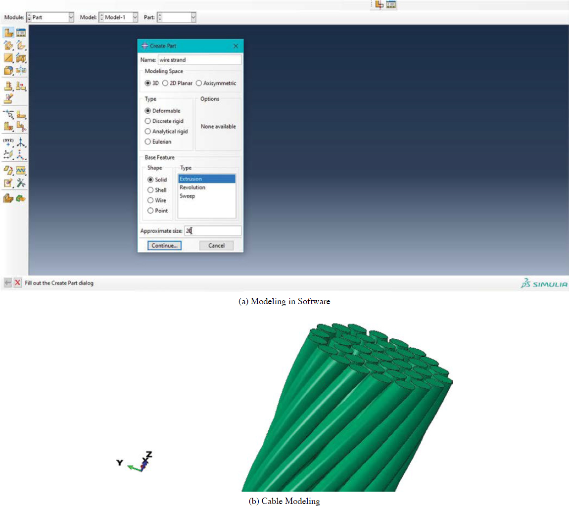
In the finite element analysis, modeling and simulations were carried out to determine cable life and provide recommendations for increasing the performance of cables. The finite element analysis deals with a multilayer strand of the construction of wires. The method of its implementation and the approach to creating the geometric model of the strand are demonstrated. To predict the behavior of the multilayer strand under tension, torsion, thermal loading, and a water environment, the geometric model was implemented in a finite element program. Software

***Figure 5.10. Eight-node linear mesh element with an integration point.***

Page 124

Suggested Citation: "5 Cable Replacement." National Academies of Sciences, Engineering, and Medicine. 2024. Transit Traction Power Cables: Replacement Guidelines. Washington, DC: The National Academies Press. doi: 10.17226/27907.

***Figure 5.11. Stress distributions for cables determined with the FEM.***

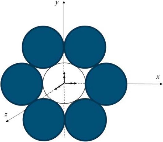
was used in the analyses. Geometric modeling was carried with a multilayer strand system. The input parameters for the studied strand were taken from the common material properties. The wire strands are considered a deformable body in a 3D solid-element definition. The geometrical model of the multilayer cable was created in the finite element environment. In Figure 5.12, finite element cable modeling in a coordinate system is presented.

In the finite element modeling, elements were modeled as shown in Figure 5.13, and boundary conditions and meshes were set as shown in Figure 5.14. In the modeling, each element was referred to as local axes X, Y, and Z, they were carried to the global system in the analyses, and the initial coordinates were kept for the strands (Alkharisi and Heyliger 2021). After modeling, meshes were defined in the software. Meshes were defined as multilayered members. Boundary conditions were also defined in the same environment. For accurate analysis results, accurate modeling and boundary conditions are needed. In cable modeling, boundary conditions vary with the location and type of the system.

In the finite element modeling, cables were modeled using structural modeling elements and techniques. Finite element software was used to assign the elements, as seen in Figure 5.13a. In cable modeling, a hexagonal shape was defined with strands, as seen in Figure 5.13b. These models are commonly used models for cables that have a meshing approach. Once the model was meshed, the next step was to assign the boundary conditions for the member. With assigned boundary conditions, the model was ready for loading. In Figure 5.14, the modeled system is

Page 125

Suggested Citation: "5 Cable Replacement." National Academies of Sciences, Engineering, and Medicine. 2024. Transit Traction Power Cables: Replacement Guidelines. Washington, DC: The National Academies Press. doi: 10.17226/27907.

***Figure 5.12. Cable modeling in a coordinate system.***

***Figure 5.13. Finite element modeling for cables.***

Page 126

Suggested Citation: "5 Cable Replacement." National Academies of Sciences, Engineering, and Medicine. 2024. Transit Traction Power Cables: Replacement Guidelines. Washington, DC: The National Academies Press. doi: 10.17226/27907.

***Figure 5.14. Meshing and boundary conditions for cables.***

demonstrated with assigned boundary conditions. With this modeling, finite element modeling was completed. During the analyses, boundary conditions were revised to demonstrate the change in structural conditions.

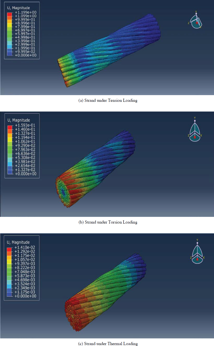
The material model was characterized by a linear relationship between stresses and strains. The displacements and strains were assumed to be small. Hence, the geometrically linear behavior of the strand and the nonlinear theories were very close in the usual practical axial load range. The assumed modulus of elasticity of the wire material was taken based on the used material properties. The wires were made of a homogeneous, isotropic, and linearly elastic material. Only the elastic region of the behavior of the multilayer strand was considered. The strand was analyzed under four different types of loading: tension, torsion, thermal, and water effect. Figure 5.15 presents tension, torsion, and thermal loading on cables.

For the analysis of cable strands with thermal loading, a specific material with conductivity, density, elasticity, expansion rate, and specific heat was considered. The analysis step was considered

Page 127

Suggested Citation: "5 Cable Replacement." National Academies of Sciences, Engineering, and Medicine. 2024. Transit Traction Power Cables: Replacement Guidelines. Washington, DC: The National Academies Press. doi: 10.17226/27907.

***Figure 5.15. Tension, torsion, and thermal loading on cables.***

Page 128

Suggested Citation: "5 Cable Replacement." National Academies of Sciences, Engineering, and Medicine. 2024. Transit Traction Power Cables: Replacement Guidelines. Washington, DC: The National Academies Press. doi: 10.17226/27907.

as a couple of temperature displacements (transients) with direct specification distribution and constant cross-sectional variation through the region. Temperature displacement analysis is a combination of heat transfer and structural stress. Due to heat transfer, there is a thermal gradient, and there is thermal expansion because of a thermal gradient.

Hence, thermal expansion causes axial stresses. These thermal effects can be applied to the system by implementing thermal diffusivity. Thermal diffusivity is explained with the thermophysical property that defines the speed of heat propagation by conduction with the change of temperature in the defined environment. The higher the thermal diffusivity, the faster the heat propagation. The thermal diffusivity is related to the thermal conductivity, specific heat, capacity, and density. This relationship can be defined as given in Equation 5.12. The quantity of heat (q) required to change the temperature can be calculated by Equation 5.13.

$α = \frac{λ}{ρ * c p}$

(5.12)

$q = m * c * Δ T$

(5.13)

Where, α = thermal diffusivity, λ = thermal conductivity, ρ = density, cp = specific heat capacity, m = mass, c = specific heat, and ΔT = temperature difference.

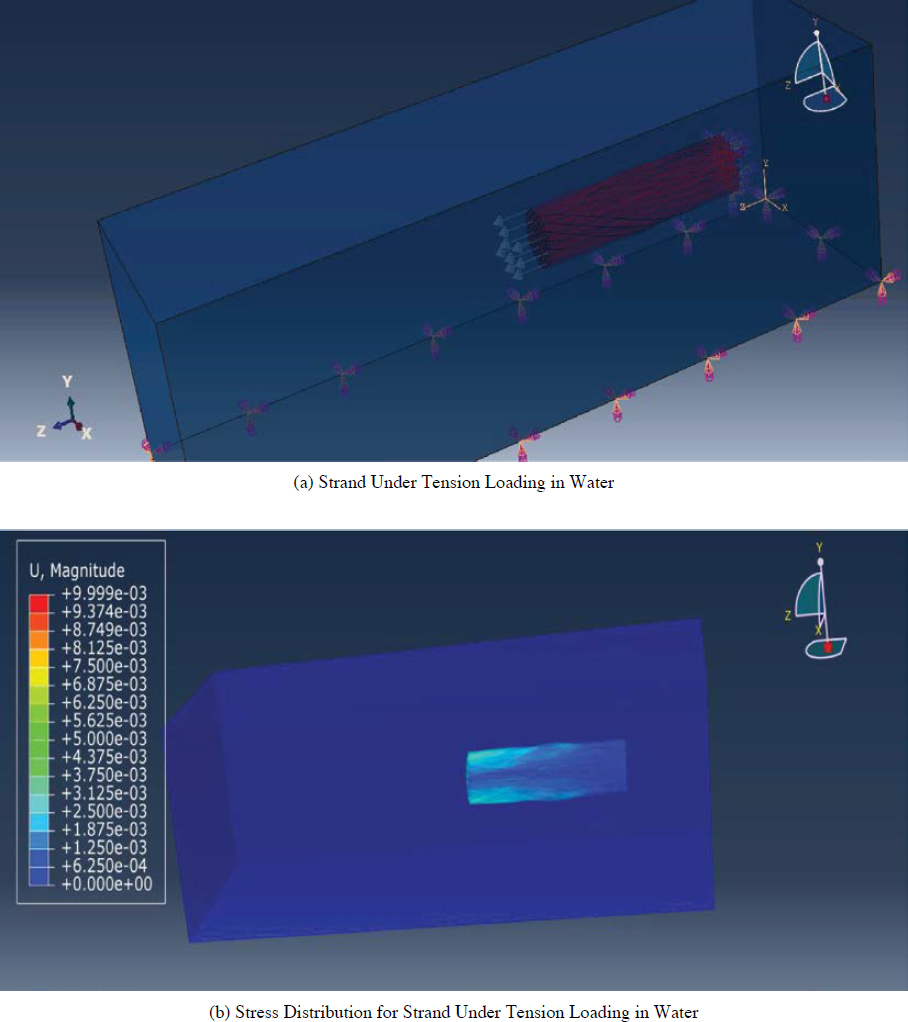
For the analysis of a wire strand underwater, the water was taken into account as an Eulerian environment, and the water density and viscosity were assigned as the U_S-U_P state with a special equation of state (EOS). After assembling and applying tensile loading for strands, a 0.2 interaction between strands was applied on the model as a surface-to-surface contact and general contact between wire strands and water. The wire strands are in the interaction of water and under the geostatic stress of water. Water pressure is defined in Equation 5.14. Figure 5.16 presents strands under tension loading in water. Definition of the pressure is important in the model. The model is created under water pressure. This water modeling is created to present the cables under water since some agencies have their cables under water because of where the agencies are located.

$P = ρ * g * h$

(5.14)

Where, P = water pressure, ρ = density, g = gravity, and h = height.

Figure 5.17 is presented with three different loadings to show the final stage of the finite element analysis. The stress distributions on cable strands under tension, torsion, and thermal loadings are presented in the figure. According to analysis results, magnitudes are presented with different stress levels. These stress levels are for the most common conditions that cables are exposed to during the construction and environmental condition changes. Therefore, cables should be investigated considering various environmental changes. These changes and stresses on cables affect the cable lifetime. To investigate the existing cables, environmental effects are demonstrated in the finite element environment. In addition, cable material change, defects, and cable aging problems can be considered accurately with the finite element approach.

5.7 Conclusions

In this chapter, cable replacement was evaluated using an optimization process and finite element analysis approach. The optimization process starts with estimating the cable failure rates. The failure rate models can be estimated using historical failure records. Each failure record

Page 129

Suggested Citation: "5 Cable Replacement." National Academies of Sciences, Engineering, and Medicine. 2024. Transit Traction Power Cables: Replacement Guidelines. Washington, DC: The National Academies Press. doi: 10.17226/27907.

***Figure 5.16. Strands under tension loading in water.***

Page 130

Suggested Citation: "5 Cable Replacement." National Academies of Sciences, Engineering, and Medicine. 2024. Transit Traction Power Cables: Replacement Guidelines. Washington, DC: The National Academies Press. doi: 10.17226/27907.

***Figure 5.17. Stress distribution on strands under tension, torsion and thermal loadings.***

Page 131

Suggested Citation: "5 Cable Replacement." National Academies of Sciences, Engineering, and Medicine. 2024. Transit Traction Power Cables: Replacement Guidelines. Washington, DC: The National Academies Press. doi: 10.17226/27907.

should include insulation type, jacket type, conduit, rated voltage, cable age, presence of water, exposure to extreme temperatures, whether underground or overhead, length of the power cable segment, the number of previous repairs on the cable, and maintenance period. With such a database, cable failure rates can be estimated accurately. Then, the optimal replacement period can be identified considering the cost of maintenance, replacement, and failures. In the optimization process, the determination of this period is important in determining the cable life. The procedure summarizing the determination of the optimal cable replacement period was given in Section 5.5. The overview of the procedure was given in Figure 5.18.

Finite element analysis was then carried out for the cables. Cables were analyzed under four different types of loading: tension, torsion, thermal, and water effect. With the finite element analysis, behavior of cables can be determined in various conditions. The conditions considered for investigation were among the most common conditions for cables. With finite element analysis, cables can be modeled accurately and their conditions and environmental and physical parameters can be defined in a simulation. This simulation can be used in the decision-making process. Especially, thermal effects can be simulated through the system to assess any heat effects on cables. Continuous change in heat can be applied on the cables as a tool of the monitoring system.