Incorporating Climate Change and Climate Policy into Macroeconomic Modeling: Proceedings of a Workshop (2024)
Chapter: 4 Economic Impacts of, Damages from, and Risks of Climate Change
4
Economic Impacts of, Damages from, and Risks of Climate Change
The purpose of this session is to review a range of approaches to estimate the economic impacts, damages, and risks of climate change to explore potential pathways for improvement. The session focused on a closer examination of the empirical relationship between climate or climate-related meteorological variables and aspects of the economy, including those that describe the macroeconomy or that may plausibly connect to inputs of parts of the macroeconomy. Earlier work of the 1990s and 2000s by William Nordhaus, Nicholas Stern, and Marty Weitzman laid out the theoretical groundwork to qualitatively consider climate change as an economic problem using mathematical models but were limited by the ability to calibrate these models to real-world data. The recent work shared in this session explored a range of novel methods to empirically measure these types of relationships with improved data availability and techniques for calibration and the implications of these relationships. These approaches included both a top-down approach, which focuses on the aggregate output of the economy, and a bottom-up or enumerative approach, which uses the microdata to estimate high-quality causal impacts of climate on each sector to integrate and sum up afterward. The presentations in this session considered the pros and cons of each approach, key insights learned, and important takeaways to inform future macroeconomic modeling development.
TOP-DOWN APPROACH
Marshall Burke, Stanford University, discussed his top-down approach to estimating physical climate risks at national and global scales. His approach examines the aggregate output of the impacts on the economy by focusing on gross domestic product (GDP), which implicitly embeds some of the costs and benefits of adaptation (e.g., sector reallocation). However, there are challenges to using GDP because of limited data for individual countries, so Burke uses global data. Moreover, GDP misses a lot of important factors, such as welfare (see Box 1-2).
Burke illustrated the top-down approach by examining whether the economy grows faster or slower during hotter-than-average years and subsequent years. He used per capita GDP growth data and temperature and precipitation data over approximately 60 years and from 190 countries to compare the economic growth rate of each country to itself across temperature fluctuations over time. The exercise established causal inferences between the
temperature fluctuations and the economic growth rate in those hotter years and subsequent years.
SOURCE: Presented by Marshall Burke on June 14, 2023.
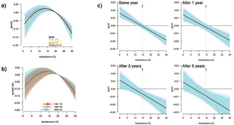
Burke’s analysis of empirical data revealed a global, nonlinear response of GDP growth to temperature (Figure 4-1a). He showed that colder to average temperature countries tend to have a positive economic growth rate with warming. In contrast, average to warmer temperature countries—where the majority of the global population resides—exhibit a negative economic growth rate as the world warms.
To study the relationship over time, Burke used 60 years of data, grouped by two-decade increments (Figure 4-1b). The data showed that there was no change in the response function over time, which implies that the world has not yet successfully adapted to warmer temperatures. He noted that the data would have shown a flattening of the response curve if there had been successful adaptation. Expanding the analysis, Burke examined the lagged response, or the relationship, between a given year’s temperature and the economic growth rate in subsequent years (Figure 4-1c). This derivative-based approach showed the cumulative negative effects of one hot year. Over time, the curve exhibited a progressively negative shift, eventually stabilizing after ~5 years.
SOURCE: Presented by Marshall Burke on June 14, 2023.
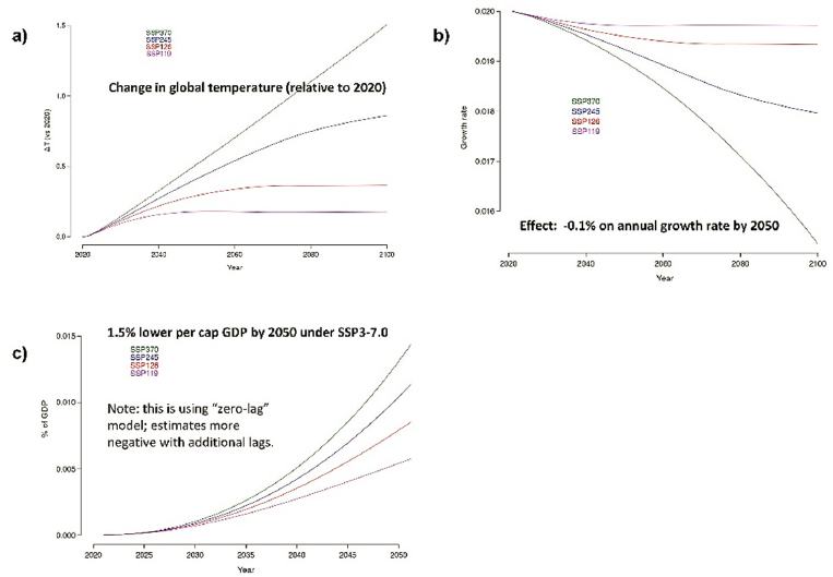
To demonstrate the implications of the immediate and lagged response curves for the near-future GDP response, Burke conducted a case study on the United States. He used temperature data from the Shared Socioeconomic Pathways (SSP) warming scenarios and assumed a conservative baseline growth rate of 2 percent and a now warming growth rate. Then, Burke input the different SSP temperatures into the response function to measure the impacts on the GDP growth rate until 2050 under each scenario (Figure 4-2). Under the business-as-usual case (SSP370), with an expected 1.5–2°C warming, the U.S. economy is expected to lose 0.1 percent of annual growth rate. Inputting the temperatures into the lagged response function resulted in 4–5 times more loss in annual growth rate.
Burke concluded his presentation with two key thoughts. First, although recent literature suggests that the economic impacts of climate are already factored into macroeconomic projections owing to historical trends in total factor productivity (TFP) growth, Burke’s GDP data suggest otherwise. His results showed that the United States has been operating at the optimum temperature in recent decades, but increased temperatures will move the United States away from this optimum, leading to a slowdown in TFP growth. This suggests that climate impacts have not been fully integrated into the future projections and will increasingly negatively affect economic growth. Second, Burke highlighted the
importance of historical GDP data as a useful empirical constraint on the relationship between economic growth and temperature. He suggested that future macroeconomic modeling work take advantage of these empirical relationships to better align models with real-world data and outcomes.
BOTTOM-UP APPROACH
Econometric Approach
Tamma Carleton, University of California, Santa Barbara, discussed her bottom-up approach to measuring climate damages to reveal insights on the inequalities of climate change. She emphasized that climate change affects different regions and populations in varying ways, with a particular emphasis on the differentiated welfare effects, and that accurately characterizing the sector-specific local-level damage informs climate policy.
Early global climate damage assessments showed an aggregate estimate of approximately 1.3 percent global economic loss per 3°C warming (Nordhaus, 1993). However, Carleton and the Climate Impact Lab, among others, are using high-spatial-resolution data to examine inequality that may be masked by this aggregate estimate (e.g., Carleton et al., 2022; Conte et al., 2021; Depsky et al., 2023; Hultgren et al., 2022; Rode et al., 2021, 2023). Carleton outlined a few prominent features of this new approach.
- Empirical foundation. Empirical work in recent decades is usually incorporated into both top-down and bottom-up damage estimations.
- Ability to integrate probabilistic projections. This work uses large ensembles of climate models to critically think about statistical and climate uncertainty in terms of the magnitude of warming and spatial distribution. Carleton noted that getting a probabilistic sense of local warming is crucial when considering inequality.
- Empirical data and approaches. This is vital to capture differential vulnerability and adaptive abilities across populations to the same climate event(s).
In short, Carleton argued that it is possible to build empirically grounded, globally representative climate damage estimates that account for inequality and uncertainty.
Carleton described the Climate Impact Lab’s and her bottom-up approach, which starts with data collection and involves constructing empirical estimates of climate damages sector by sector. The sum of those is input into an integrated analysis of an aggregate estimate of damages (e.g., the social cost of carbon) over a given period.
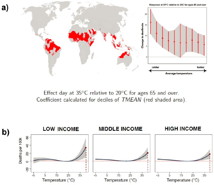
Their process includes building empirical dose-response functions to see how the impacts of each sector vary with temperature. To explore aspects of differential vulnerability, they allow for this curve to vary based on local conditions, both physical (e.g., average temperature) and economic (e.g., income levels), that serve as resources to facilitate adaptation. For instance, using mortality as an example, they showed that mortality rates vary with local mean temperature (Figure 4-3a), where colder regions are more sensitive to extreme heat and hotter regions less sensitive. Factoring in the influence of economic
resources, Figure 4-3b shows that mortality rate is more sensitive to extreme heat in lower-income regions and less sensitive in higher-income regions.
SOURCE: Presented by Tamma Carleton on June 14, 2023.
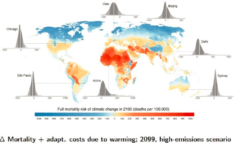
Carleton explained how her team combined these dose-response curves with ensembles of climate model projections to estimate climate change damages in each sector, while accounting for the varying responses across regions to climate change. She explained that a main advantage of this approach is that it provides a full distribution of projected impacts for each location (Figure 4-4). By examining sectoral impacts across income and temperature deciles, they found that mortality damages are primarily experienced by today’s global poor. However, adaptation spending to mitigate mortality risks are mostly borne in today’s wealthiest populations (Figure 4-5).
SOURCE: Presented by Tamma Carleton on June 14, 2023.
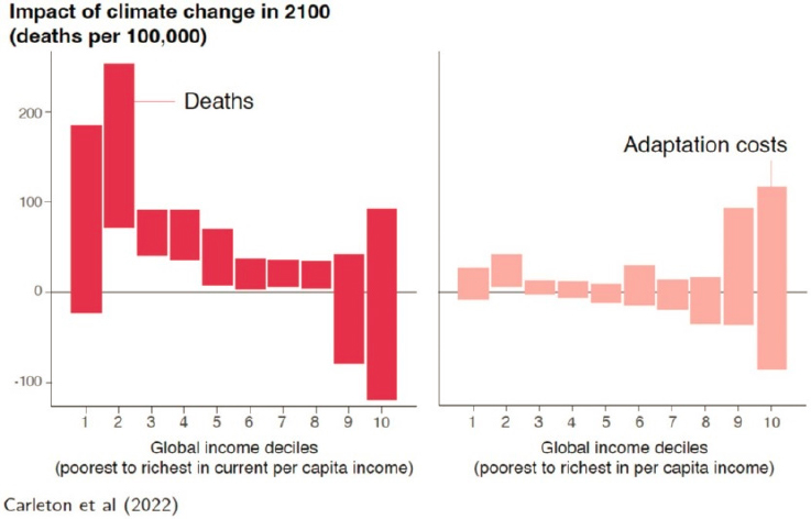
SOURCE: Carleton et al. (2022)
When Carleton and her team applied their approach to each sector, they showed different patterns of inequality compared to mortality risk. For example, she observed that agricultural losses are greatest in warmer, wealthier regions (Hultgren et al., 2022), while labor losses are sector dependent with industries more exposed to climate change suffering greater losses (e.g., agriculture, mining, and construction) (Rode et al., 2023). Lastly, Carleton showed that income is critically important in the energy sector (Rode et al., 2021), primarily affecting wealthier regions.
To calculate aggregate damages, Carleton integrated the extreme spatial heterogeneity into the SCC calculation. This involved computing a spatial certainty equivalent damage function, placing a higher weight on damages in poorer regions to reflect the increased marginal utility of a dollar in these regions compared to wealthier regions. This accounting for inequality led to dramatic increases in damages relative to those in scenarios that ignored inequality.
In summary, Carleton’s bottom-up approach demonstrated that nonmarket damages are a significant component of the aggregate damages of climate change, with nonmarket damages from labor and mortality dominating the overall number (Rennert et al., 2022). She identified three main challenges in incorporating sector-specific damages into aggregate damage functions: (1) converting physical units to monetary units, (2) accounting for feedbacks and interactions, and (3) understanding the role of migration in characterizing location- and sector-specific damages.
Process-Based Modeling Approach
Jeremy Martinich, U.S. Environmental Protection Agency (EPA), discussed the Climate Change Impacts and Risk Analysis (CIRA) Project,3 which aims to quantify climate impacts to provide useful information for users on how their lives may or may not be benefited by greenhouse gas (GHG) mitigation and adaptation actions. CIRA predominantly uses a bottom-up, process-based modeling approach to assess how climate affects sectors (e.g., human health, infrastructure, and ecosystems) in the United States. However, this approach involves coordination among modeling teams and time to rerun the models for each new question.
To reduce these complexities, EPA developed a simplified version of the CIRA Project called the Framework for Evaluating Damages and Impacts (FrEDI)4,5. Martinich explained that they use CIRA’s detailed, bottom-up, high spatial and temporal resolution modeling of sector-specific impacts to create damage functions for FrEDI. Figure 3-6 outlines the sectoral coverage that FrEDI includes, which is comprehensive but not complete. Additionally, the model only captures U.S.-specific impacts; relevant global impacts are not captured.
Martinich explained that FrEDI enables the user to examine what total damages may look like and their distribution across sectors at the aggregate level, nationally, regionally,
___________________
3 See www.epa.gov/cira.
4 See https://www.epa.gov/cira/fredi.
5 FrEDI is open source and transparent. It is available on GitHub (www.github.com/usepa/FrEDI).
or by impact type. He also said that the model can help users assess the likelihood of certain populations facing greater risk based on race and ethnicity. One main challenge in Martinich’s work is connecting physical climate impact modeling to the macroeconomic models, such as the Macroeconomic Advisers U.S. Some impacts captured in FrEDI are not directly relevant to capital or other effects with straightforward connections to the flows represented in macroeconomic models.

SOURCE: Presented by Jeremy Martinich on June 14, 2023.
Martinich closed with a few key takeaways. He emphasized that future work is needed to connect the sector-level physical climate impacts modeling, such as in FrEDI, with macroeconomic models. He noted that the model currently underrepresents extremes, partly due to the underrepresentation of extremes in physical climate models’ projections and their focus on means and medians. He also said that expanding the modeling to capture global distributional effects will improve the model’s utility and coverage. And finally, Martinich encouraged the Roundtable to expand the scope of the macroeconomic budget considerations beyond the typical 5- to 10-year horizon. He highlighted that climate science typically focuses on longer timescale trends, as the level of warming projected by mid-century and later is much larger than what will be experienced in the near term. Expanding the time frame for economic assessments can facilitate collaboration with climate science and improve understanding of any impending changes in rate of damages over a longer time frame.
DISCUSSION
The following panel discussion explored the advantages and disadvantages of the presented approaches and discussed potential pathways for improved ability and utility. First, the panelists discussed the extent to which adaptation is captured in their approaches. Burke explained that the top-down approach assumes that the net effect of adaptation should already be implicitly captured in the estimates. He reiterated that his study’s results suggested that adaptation is slow and costly based on historical data, as responses to climate change have not flattened over time. In contrast, Carleton suggested a more optimistic outlook on adaptation, highlighting that their bottom-up approach captured historical adaptation to some extent. However, she warned that their bottom-up approach is not able to capture large technological shifts in adaptation and that some sectors were more difficult to model than others (e.g., migration). Martinich mentioned that the bottom-up approach of the CIRA Project considers adaptive responses of populations to come up with the most accurate estimates. For example, to estimate the effects of high-tide flooding and road infrastructure, the model considers that if a road is flooded, travelers will adapt to find an alternative route to continue with their commute. Martinich said that capturing more complex adaptive response (e.g., migration) is an active area of research. This is happening both at the CIRA level within U.S. borders, but also in the work of other research groups at the global scale.
Next, the panelists discussed the challenge of distinguishing a signal from natural noise of climate variability on a 5- to 10-year timescale given the increasing frequency and magnitude of climate-related events. Martinich explained that time is both a disadvantage and an advantage. He noted that because GHGs are long-lived, globally mixed pollutants, time is required to observe policy effects and climate system responses. One participant pointed out that natural variability exhibits distinct phases and coexists with secular trends. While these can be separated in the historical record, predicting their combined future impact is challenging. However, studying specific historical events can isolate natural variability and simplify the problem, improving understanding of their effects and frequency. Carleton added that her current statistical modeling work explores various case studies within a larger dataset to extract statistical relationships and parameterize parts of the response curves that can be sampled to look into the future.
Burke addressed the question of how to use the historical record without getting overly anchored, given the nonlinear relationship between climate impacts and temperature. He explained that nonlinearities are present in both the climate system’s response to forcing and social systems’ response to climate change. He said that climate scientists focus on the former, while economists focus on the latter to estimate future scenarios based on these nonlinearities. Burke noted that historical data are more useful for predicting the future in some sectors, such as mortality response to temperature. In contrast, Rachel Cleetus, Union of Concerned Scientists, mentioned that the nonlinear physical impacts of wildfires on insurance and reinsurance lack sufficient historical precedents. She emphasized the importance of understanding market and policy incentives to adequately address rapidly in-
creasing climate impacts. Carleton added that improving data collection of diverse locations, landscapes, and populations and enhancing communication of attribution science can aid in exploring the nonlinearities of the climate and social response to climate change.
James Rising asked about the next steps for FrEDI. Martinich outlined that the pathway forward can combine the strengths of econometric and process-based approaches. The first objective at the EPA is to improve the comprehensive characterization and inclusion of climate change impacts in the FrEDI model. Simultaneously, both the econometric and process-based modeling approaches, which are partially integrated into FrEDI, can be intentionally overlapped more to gain further insights into structural uncertainty. Martinich stated that there is room within each sector to improve their estimation, and this can benefit from improved empirical understanding from econometric approaches and better representation of processes in the model.


