Incorporating Climate Change and Climate Policy into Macroeconomic Modeling: Proceedings of a Workshop (2024)
Chapter: 3 Research Landscape
3
Research Landscape
Expanding on the previous two sessions, this session delved deeper into a more research-oriented perspective. The session moderator, Adele Morris, Federal Reserve Board of Governors, explained that there is overlap in applications and principles between models used at the federal level and research models. Both use models to ask a question and explore potential outcomes. Lars Peter Hansen, University of Chicago, and Peter Wilcoxen, Syracuse University, presented their research to help workshop participants think through how long-run economic growth can depend on how the nation addresses the climate challenge. Additionally, Wilcoxen discussed the range of potential transition outcomes.
COMPUTATIONAL GENERAL EQUILIBRIUM MODELS
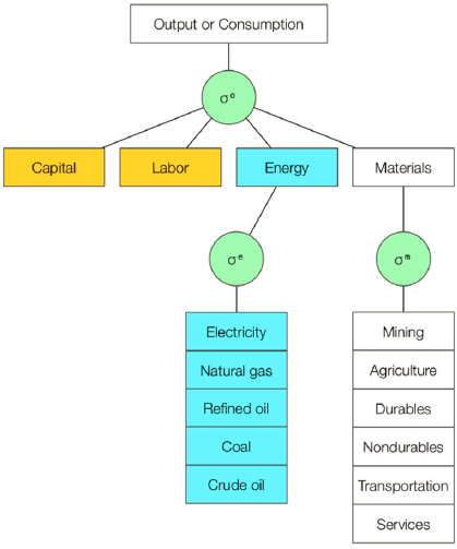
Wilcoxen discussed computational general equilibrium (CGE) models, a type of economic model that has been extensively used to analyze climate and energy policies. He explained that the primary characteristic of these models is that they typically segment the economy into distinct producing and consuming sectors. To illustrate this, he used the G-Cubed Global Model, which divides the world economy by region and then subdivides it by various actors, including 20 producing sectors, households, investors, and the government. Each of the producing sides of the economy is further divided into subsectors, with many linked to the energy sector. Wilcoxen noted that CGE models vary in their economic focus, and there is no single model for all purposes, as emphasized by James Stock in the opening keynote.
Figure 3-1 displays the inner workings of a single region in G-Cubed. The left side lists the markets, dividing the economy’s producing side into the 20 individual sectoral markets in G-Cubed model, each in a row. The bottom two rows are primary factors: labor and capital. These are supplied by households rather than individual firms. The columns represent buyers and sellers in the economy (together referred to as agents). The first 20 are the producing sectors and the remainder are final demand sectors: household consumption, investment, the government, exports, and imports.
Wilcoxen highlighted a key feature of CGE models: The agents interact in many markets and their behavior jointly determines the prices that balance supply and demand simultaneously in all of the markets. Each agent’s behavior is mathematically modeled (depicted in Figure 3-2) based on each agent’s objective (e.g., minimizing cost, maximizing utility). The agents determine how much of each input to buy based on the prices they face and how willing they are to substitute one input for another, shown by the green circles in
the schematic representing substitution elasticities. These elasticities, along with other historical information, capture how agents respond to policies, especially price changes.

SOURCE: Presented by Peter Wilcoxen on June 14, 2023.
SOURCE: Presented by Peter Wilcoxen on June 14, 2023.
Wilcoxen described the application of these models to study different environmental and climate policies. He said that one way to introduce climate impacts into the models is by adjusting industry productivity, such as reducing agricultural output to simulate decreased precipitation. He explained that the models have also been used to look at other kinds of environmental impacts, such as air pollution affecting mortality rates and consequently altering population and labor dynamics. Lastly, Wilcoxen mentioned efforts to include environmental amenities in household utility functions to reflect how individuals value an improved environment for their benefit.
Wilcoxen emphasized the crucial role of behavioral connections across time when considering climate. Many CGE models used to study climate policy have forward-looking agents, which are households or firms that consider the impact of their investment decisions on future cash flows. Additionally, these CGE models examine how current household consumption and savings choices influence future utility and consumption capacity. Wilcoxen stressed that this is extremely important for climate modeling because of the intertemporal nature of investment and savings decisions, particularly related to how agents respond in the near term to anticipated future changes in climate conditions or economic policy. For example, when considering incentives such as those in the Inflation Reduction Act (see Chapter 5), Wilcoxen emphasized the importance of assessing whether agents will remain engaged and continue to uphold the incentives. If not and people do not believe that the incentives will be there, agents will not invest because they are forward-looking and think the policy may not last.
Wilcoxen said that CGE models usually do not assume exogenous gross domestic product (GDP) growth but instead build it from its constituent components, either by considering income (i.e., summing returns to labor and capital) or expenditure (i.e., summing the value of final demand). He highlighted the common drivers of GDP growth, such as labor force growth, capital formation, productivity, terms of trade, and the employment rate, and noted the significance of factor mobility, referring to the movement of factors of production (e.g., labor, capital, or land) between both regions and industries. Immobile factors can result in lasting policy costs due to their slower adaptation to shocks. For example, if labor is fixed in specific industries and locations, policies can create long-lasting costs because people cannot easily move to new industries. Similarly, immobile physical capital, typically tied to specific regions or sectors, presents challenges as relocating equipment and machinery leads to significant capital losses. As such, Wilcoxen stressed that factor mobility is crucial when modeling the short-term impacts of policies on GDP.
Wilcoxen explained that the G-Cubed model blends key elements of macroeconomics with general equilibrium modeling. It stands out from typical CGE models because it includes uncommon features, including:
- Mix of intertemporal agents: Some agents possess foresight, while others do not. This feature aids in simulating how people adapt to real-world policies.
- Sector-specific capital stocks: This feature reflects the challenge of moving capital into or out of an industry (e.g., transitioning a coal plant into a solar farm).
- Detailed treatment of financial markets: The model tracks equity in each sector, government and international debt, foreign currencies, money supply, central bank policies, and asset risk premiums.
- Slow adjustments in nominal wages: The model allows for short-term disequilibrium in labor markets.
- Comprehensive bilateral trade: Wilcoxen reminded workshop participants that climate is a global problem and that policy in other countries can affect the United States.
Wilcoxen presented a practical application of the G-Cubed model to demonstrate its utility. He showed the results from a simulation that examined the effects of reduced productivity in durable manufacturing 5 years in the future. Wilcoxen highlighted that the durable sector was the most affected (Figure 3-3a), due to reduced productivity leading to increased prices, reduced demand, and harm to the U.S. economy given that durables are a significant export. Consequently, Figure 3-3b shows the labor impacts in Year 7. Wilcoxen highlighted the cascading effects from the durables sector’s productivity decline. Even though the services sector was less affected by productivity decline, he explained that it employs a significant portion of the U.S. workforce, so it accounts for a large share of job losses. He emphasized that climate action is at the individual sector and regional level rather than the macro level. His results showed that there will be significant consequences due to changes in productivity and prices at the micro level, while macro-level impacts on GDP may be small.
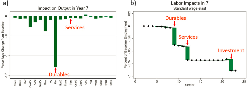
SOURCE: Presented by Peter Wilcoxen on June 14, 2023.
However, Wilcoxen emphasized the inherent uncertainty in these models, even when constructed with great care, extensive data, and advanced econometrics techniques. He illustrated the issue using a set of parameters related to household consumption behavior in the intertemporal general equilibrium model, a 35-sector model of the United States. These
parameters have significant standard errors due to limited data from World War II; the results are thus imprecise, which would be true of any statistical model, but importantly for examining macroeconomic impacts, the errors do not necessarily average out across sectors. Wilcoxen then discussed how the covariance matrix of the model’s parameters can be used to calculate standard errors for the model’s results. Using the standard errors, he showed the degree to which several of the models’ outcomes were affected by uncertainty in both consumption and production parameters. In addition, he noted that other sources of uncertainty, such as exogenous variables, the form of the model’s equation, or climate uncertainty, were not considered in this analysis.
Wilcoxen’s covariance matrix produced standard errors for the output for various industries, using percentages of the corresponding base case value. For example, crude oil output had a standard error of 40 percent, primarily due to production uncertainties. Additionally, he presented a decomposition analysis that distinguished between the impacts of uncertainties in modeling household consumption and those in production. Similarly, he analyzed the uncertainties in macroeconomic variables. Wilcoxen highlighted that the standard error for predicting overall consumption at the macro level based solely on parameter uncertainty is 4 percent of the baseline value, but that predicting carbon emissions is substantially less certain, with the standard error exceeding about 13 percent of the baseline value. While many models report a single trajectory for these variables, he said that there are significant uncertainty bands around these predictions, highlighting the challenges in precise forecasts.
Wilcoxen concluded his presentation on a positive note, stating that despite uncertainties in the parameters, the model’s results show that climate policies—specifically, a carbon tax with a particular revenue recycling assumption—would be effective. He explained that climate policy leads to a clear decline in the coal industry. Importantly, in the scenario he presented, the economy’s overall capital stock would increase due to cuts in capital taxes funded by carbon tax revenue. However, the impact on other sectors, such as agriculture, remains much less certain and depends on how people adapt to energy price changes. Wilcoxen also highlighted challenges in research needs, including the need for detailed energy-sector data and geographic information for accurate climate impact modeling. He stressed the importance of linking models and developing protocols to understand how highly spatially detailed climate impact models interact with broader macroeconomic models with lower spatial resolution. Lastly, Wilcoxen advised against overselling results and urged considering the scale of changes relative to the noise in the modeling process.
UNCERTAINTY QUANTIFICATION
Hansen opened his talk by quoting Rising et al. (2022): “The economic consequences of many of the complex risks associated with climate change cannot, however, currently be quantified.… [t]hese unquantified, poorly understood and often deeply uncertain risks can and should be included in economic evaluations and decision-making processes.” While sympathetic to this challenge, Hansen said that the challenge is to provide the tools to address it. He said that acknowledging the limits of scientific understanding is the real
challenge for quantitative policy analysis. To make a broadly based notion of uncertainty operational, Hansen also defined three components of uncertainty, detailed in Box 3-1.
BOX 3-1
Hansen’s Key Definitions
Hansen defined three components of uncertainty during his presentation. First, he used risk to define unknown outcomes with known probabilities. He described one source of risk inside models as the shocks that modelers put in models that are specified with probability distributions. Hansen used ambiguity to define unknown weights to assign to alternative probability models. He explained that when there are multiple models to choose from and to use, experts may want to look across multiple models when there are situations of uncertainty. This typically cannot be resolved from historical evidence and requires subjective inputs. Thus, there is uncertainty about the subjective prior inputs. Lastly, Hansen also used misspecification, also known as likelihood uncertainty, to describe unknown ways in which a model might give flawed probabilistic predictions. Of the three components of uncertainty that Hansen defined, he expressed that misspecification is the most difficult to understand yet may be the most important.
Hansen noted that it is critical to establish a flexible framework that enables more precise uncertainty quantification for dynamic economic models. His research strives to develop tractable methods for assessing the impact of uncertainty on climate policy outcomes and isolating the most significant sources of uncertainty. He employs probability models that allow for misspecification and ambiguity to conduct extensive sensitivity analyses with statistical tools that refine and constrain the forms and amounts of uncertainty. He emphasized the importance of considering aversion to uncertainty, particularly in policy discussions. Instead of prescribing a specific level of aversion for decision makers, Hansen’s work focuses on explaining the consequences of different aversions to policy outcomes. One notable set of outcomes of his research is uncertainty-adjusted probability measures, which aid robust decision making by helping to determine the appropriate level of uncertainty aversion along with identifying the components of uncertainty that matter most to decision making.
To illustrate implications for uncertainty quantification, Hansen said that there are three main sources of uncertainty in understanding of the potential climate change impacts: geoscientific factors related to carbon dioxide emissions, economic factors affecting opportunities and social well-being, and the research and development (R&D) including investments that could lead to economically viable clean technologies. The methods he described in the illustrative analysis identified the third channel as the most significant one for shaping policy questions and potentially closing knowledge gaps.
Next, Hansen discussed how to confront the challenge of implementing prudent climate policies amid uncertainty around timing and severity of environmental damage. He
studied how a decision maker addresses uncertainty when balancing immediate action versus waiting for more information. For example, investments in R&D could speed up the discovery of green technologies, but there is a risk component and more extreme shocks that can affect uncertainty.
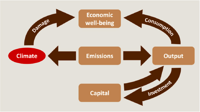
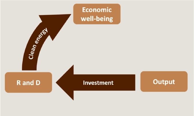
Hansen presented a standard model with climate change as an externality (Figure 3-5). Capital produces output, which can be divided between investment and consumption. Increased emissions are associated with more energy input into production, increasing output. However, emissions can affect the climate and lead to costs to economic well-being. Hansen said that the left-hand side of the model is where market failures appear. Lastly, he incorporated the possibility of R&D investment (Figure 3-6), which may generate new clean technologies and therefore improve economic well-being.
Hansen outlined three channels of uncertainty that he studies: (1) emissions impact on climate, (2) climate impact on economic damages, and (3) returns to investment in new green technology. He explained that the research community needs better and richer inputs, which is possible but must be done in a tractable way. He then presented his method for uncertainty quantification.
First, Hansen showed a histogram of the baseline distribution of climate sensitivities, using data from ~144 different climate models (Figure 3-7; shown in red). In the baseline, emissions’ impact peaks around 10 years and then stabilize. However, after assigning different weights to allow for model uncertainty, the distribution shifts to the right, with variations for less and more uncertainty aversion (Figure 3-7; shown in blue). Hansen said that the more aversion there is, the more he shifts the distribution, noting that this adjustment was made cautiously due to uncertainty about model weightings.
SOURCE: Presented by Lars Hansen on June 14, 2023.
SOURCE: Presented by Lars Hansen on June 14, 2023.
Next, Hansen presented a stylized model depicting possible damage trajectories, ranging from conservative (e.g., Nordhaus) to extreme (e.g., Weitzman) estimates. In his model, he allowed for uncertainty in the damage trajectory curvature and the potential for significant events triggered by crossing a threshold. These events would cause more environmental damage, from which they would learn more about the damage trajectory curvature. These significant events are modeled as Poisson events, allowing for the likelihood of these events in the future to be linked to temperature. The model also considered significant events such as the realization of the emergence of new green technology resulting from continued scientific R&D investment.
As with the distribution of climate sensitivity uncertainty, Hansen highlighted uncertainty in the damage curvature, with less and more uncertainty aversion compared to a baseline scenario. The baseline scenario considered 20 different curves and treated them all as equally likely. Hansen then used different weighting of these curves under more and less aversion. Hansen discussed the influence of aversion on adjustments to the social value of R&D. Neutrality (the lack of aversion) imposes baseline probabilities. He then showed modest upward adjustments with less aversion and more significant adjustments with more aversion.
After laying out his approach, Hansen emphasized the need for stochastic simulations in addressing uncertainty as he revisited the three key sources of uncertainty. He illustrated this with examples from his work, using simulated pathways of varying levels of uncertainty aversion to demonstrate the impact of uncertainty. He highlighted that technology-related uncertainty had the most impacts under modest aversion compared to climatic or economic damage uncertainty. Hansen’s research revealed that uncertainty, particularly in technology-related factors, significantly influenced R&D investments, social cost of global
warming, and carbon emission trajectories. He showed that technology-related considerations and uncertainty are crucial for decision making related to climate change, R&D investments, and carbon emissions reduction. In closing, Hansen emphasized that understanding and addressing uncertainty sources can enhance the effectiveness of economic policies, as reflected in the social cost of global warming and the prudence of R&D investments in green technologies.

SOURCE: Presented by Lars Peter Hansen on June 14, 2023.
DISCUSSION
In the open discussion, Morris asked about some of the skepticism about CGE model projections related to uncertainties in emerging technologies, their costs, and the timing and scale of their adoption. She asked the speakers how they address this skepticism and when technology uncertainties become significant in their modeling. Both experts highlighted the importance of addressing technological uncertainties. Wilcoxen mentioned incorporating productivity growth from historical data and literature estimates in his models. He also discussed addressing concerns about future differences with scenario and sensitivity analyses. Hansen discussed his focus on the development of new green technology and how he factored in an abrupt discovery with significant R&D efforts. His team considered the probabilistic success of such technology and the possibility of misspecification in their modeling.
Heather Boushey, Council of Economic Advisers, discussed the challenge of aligning economic models with the real-world complexity of policymaking in the context of the transition to a low-carbon economy. She posed two key questions. First, she asked about the difficulty of using economic models to provide policymakers with decision-making information, particularly in the face of varied sector impacts from the energy transition. Wilcoxen highlighted the importance of clearly communicating that small average macroeconomic impacts can mask significant micro-level impacts. Hansen emphasized studying heterogeneous climate-related effects across regions and countries.
Second, Boushey asked about the complexity of real-world policy implementation compared to the simplified policies that are often modeled. She mentioned that in practice, policymakers adopt a range of intricate policies, especially when implemented across multiple sectors in combination. Wilcoxen suggested incorporating sectoral and technological detail into models and coordinating across government agencies to avoid unintended consequences, particularly when climate policies intentionally raise the cost of energy. Hansen highlighted the importance of incorporating uncertainty into policy discussions and mentioned that his approach puts uncertainty inside the policy problem rather than treating it as an external factor.
One participant asked about how the G-Cubed model’s labor-sector disequilibrium impacts other sectors. Wilcoxen explained that they track income and spending across the economy and seek an equilibrium set of prices in all other markets, given the distribution of income. Thus, they reach an equilibrium that accounts for unemployment in the labor sector while maintaining consistency and balance across all sectors.
Several participants touched on a desire for more detailed economic models, the consideration of climate-related impacts on sectors such as agriculture and migration, and the limitations in current models for complex policy questions. Wilcoxen explained that, currently, most economic models do not consider regional migration as an endogenous process, even in the context of climate change. While it could be added to the model, Wilcoxen said that most models treat population as immobile between regions, regardless of climate change impacts. Hansen noted ongoing efforts, such as by Esteban Rossi-Hansberg, Uni-
versity of Chicago, and his collaborators, to incorporate endogenous migration as a response to climate change into models, but highlighted challenges in cost structures and assumption about relocation. He also mentioned his models examining the reallocation of production in the Brazilian Amazon due to climate policy responses but emphasized the need for further research on the spatial aspects of climate-induced migration.
Robert Kopp, Rutgers University, asked about the limitations of existing economic models in addressing climate change and policy responses. Wilcoxen acknowledged that GDP may not adequately reflect climate impacts and policy outcomes, emphasizing the challenge of developing more detailed models that can capture a broader range of consequences beyond GDP growth. See Box 1-2 for a longer discussion. Hansen stressed the importance of moving beyond misspecification to address uncertainties in climate modeling. He also highlighted the computational challenges of incorporating geographical and sectoral details into models, noting the potential of machine learning methods. Both speakers agreed on the importance of enhancing economic models to better address the complexity of climate change challenges.


