Evaluating Traffic Safety Campaigns: A Guide (2025)
Chapter: 6 Observational Studies

CHAPTER 6
Observational Studies
Observational studies can be effective tools for evaluating the impact of driving safety campaigns by allowing researchers to systematically observe and document driver behavior in real-world settings. These studies involve positioning trained observers and cameras, or using existing data-collection infrastructure at specific locations, such as intersections or school zones, to record behaviors relevant to the campaign. By conducting observations both before and after a campaign, researchers can detect any shifts in these behaviors, providing a direct measure of the campaignʼs effectiveness. Observational studies also allow for analysis of how driver behavior varies across different conditions, such as time of day, weather, or traffic volume. This method provides an unobtrusive, cost-effective way to gather reliable data on driver compliance and risk-taking, offering clear indicators of whether the safety campaign has achieved its desired impact on public behavior. The quick reference guide for using the observational study costing tool is available in BTSCRP Web-Only Document 7.
Staffing
Staffing salaries in the salary role table were calculated from rounded averages based on state and national employee salary numbers. Salaries for each role are found in Cells O3–O7 in the Observational Study Costs tab (Tab 5) of the costing tool workbook (Exhibit 6.1). These cells are then divided by total work hours in a year (Column P), to find the unloaded hourly rate (Column Q), which is calculated into the fully loaded hourly rate (Column S based on a multiplier/discount (Column R). The multiplier/discount is used to calculate fringe benefits or other costs incurred for salaries. The calculated salaries are then automatically applied to the times generated in the main spreadsheet to generate costs in Column H, which are then automatically added and input into the cost breakdown table located in Column M, Rows 24–29 (Exhibit 6.2).
The following are explanations of roles shown in Exhibits 6.1 and 6.2.
- Project Director. In observational studies, the project director leads the projectʼs strategic design, making sure that observational methods align with the studyʼs goals and ethical standards. They set objectives for real-time or video-based data collection and coordinate with stakeholders to ensure study goals are met. The director is also responsible for planning the scope and timeline of data collection across multiple locations and establishing risk management protocols to ensure researchersʼ safety and the quality of observational data.
- Project Supervisor. The project supervisor manages the logistics of observational data collection, from location scouting to coordinating researcher schedules and managing task assignments. They oversee the day-to-day activities of data collectors, making sure that protocols are followed consistently. The supervisorʼs responsibilities also include ensuring data quality through routine interrater reliability assessments, like Cohenʼs Kappa, to maintain consistency in behavior observation and coding.

Long Description.
The column headers under columns L through S are role, responsibilities, annual average or hourly wage, total work hours in a year, unloaded hourly rate, multiplier or discount, and fully loaded hourly rate. The data are given from rows 3 to 7.
- Project Administrator. In an observational study, the project administrator ensures logistic support is in place, managing scheduling, transportation arrangements, and the organization of study materials. They handle communication across the team and maintain organized records of project milestones, tracking progress across multiple observation sites. Their work ensures all necessary materials, permissions, and schedules are in place for smooth, uninterrupted data collection. The project administrator is given an estimated 1 hour of work per task to maintain budget and project tracking tasks.
- Project Associate/Team. Project associates assist with data collection, working directly at observation sites to record behaviors and document environmental factors that might impact data. They are trained in specific data-collection protocols and might use various recording
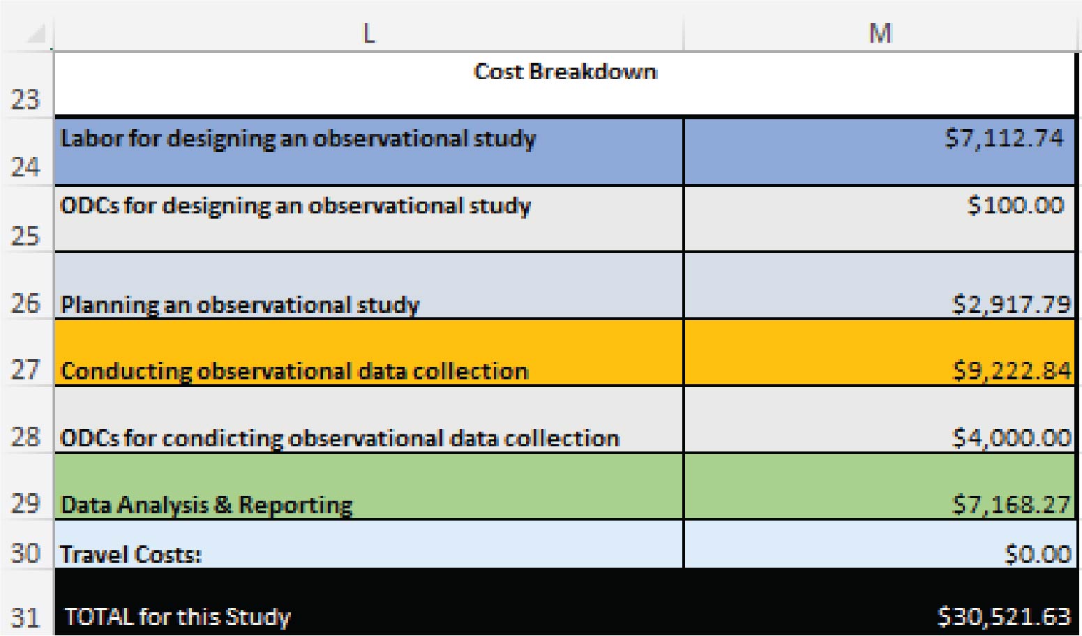
Long Description.
The column header is a cost breakdown. The data are given from rows 24 to 31. The total for the study provided in row 31 is 30,521.63 dollars.
- tools, like digital counters or cameras, to capture detailed observations. Project associates are also responsible for preliminary data transcription and organization, assisting in maintaining data accuracy and completeness.
- Data Processing Team. The data processing team prepares and organizes raw observational data for analysis, ensuring data quality and compatibility with analytical software. They conduct data validation processes, performing quality checks to remove inconsistencies or errors. This teamʼs role is essential for transforming field notes, videos, and observational records into a structured format suitable for analysis, particularly when multiple researchers are collecting data across various sites.
Other Direct Costs
ODCs include non-travel, non-labor costs for the study, and are calculated based on user inputs in Column N, Rows 10 and 11 (Exhibit 6.3). For observational studies, this includes study material costs such as pens, paper, and other consumables (N10), and if applicable, the cost of cameras (N12). The number of cameras per site (N12) and the number of locations (N5) are also used to determine the total cost for cameras if the observational study is video-based.
Travel
Travel costs for observational studies can vary depending on factors like distance from the researcherʼs location. The observational study data collection in a location away from researchers will undoubtedly require travel. However, distance and other factors can dictate what mode of transportation is needed, which can affect cost greatly. Options like airplane flights or renting cars might incur greater costs, while trains, buses, or personal vehicles might reduce costs. Depending on the governing body or business policies, the company might be required to pay mileage or other costs for researchers taking a personal vehicle. In addition, employers might be required to pay for the meals of researchers, which can vary based on which meals are covered, how many meals are covered, and location of the observational study.
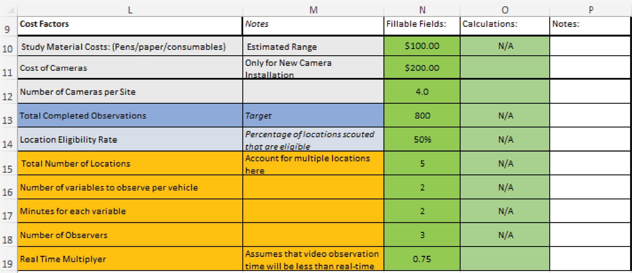
Long Description.
The column headers from columns L through P are cost factors, notes, fillable fields, calculations, and notes. The data are provided from rows 10 to 19.
To use the costing tool, a variety of fields must be filled out. Costs like lodging (per day), ground transportation costs (rideshare, bus, parking fees, or other transportation costs), and per diem costs must be input into the costing tool. These costs, where applicable, are then multiplied by travel days, workdays, and number of team members to create travel costs.
Observational study details for real-time data collection like duration of observations, number of locations, number of observations, and number of researchers will also increase travel costs. Increasing any of these variables can exponentially increase costs as additional time and hotel rooms might be required to house researchers and more time is needed to complete the required repetitions. Travel-related expenses include items such as lodging, ground transportation, and per diem rates, in the travel sections provided in each study type sheet. Costs for overnight travel to destinations greater than 50 miles can be input in Rows 34–43 of Columns B–G as described and shown in (Exhibit 6.4):
- Destination/Trip (Column B): Location of travel destination.
- Lodging Costs (Column C): Cost of hotel, or other overnight accommodation.
- Per Diem (Columns D/E): Number of days for the trip.
- Travel Days (Column D): In most cases this will be two, assuming that the traveler will be returning to the location of origin.
- Work days (Column E): Number of days in which data collection is planned (not counting travel days if there is overlap).
- Mileage reimbursement rate (Column F): This should be a set rate, likely matching the rate listed on the U.S. GSA website for domestic travel.
- Number of Team Members (Column G): How many people are traveling?
The travel values input will be used to calculate the total travel cost for each trip in the corresponding cell in Column J. The total for all trips will be combined and reported in Cell P38. Travel expenses for local trips (trips less than 50 miles) are calculated based on user inputs on the on-site observations (5A) tab of the costing tool workbook (Exhibit 6.5). The input values used are as follows:
- Mileage reimbursement rate (Cell B42): Expected reimbursement rate per mile, likely matching the rate listed on the GSA website.
- Commute time (Cell B36): Total amount of time in hours per observer to commute to and from the observation site.
The total mileage, tolls, and parking are calculated in Cell B43, assuming that the average speed of travel is 45 miles per hour, and 10% of the mileage reimbursement cost will be added for tolls and parking. The values for the assumptions in this formula may be adjusted as needed.
The total travel cost per observer is multiplied by the number of observers and total number of sites, which are input by the user on the observational study cost (5) tab in Cells N15 and N18, respectively (Exhibit 6.3). The total computed value based on these inputs is reported in Cell S17 of the same tab (Exhibit 6.6).
Observational studies within the context of a driving safety campaign involve monitoring driver behaviors directly through methods such as live observation or video recording at targeted roadways. By strategically placing observers or cameras, researchers can evaluate specific driving behaviors relevant to the campaign—such as seatbelt usage, adherence to speed limits, or the prevalence of distracted driving. These studies allow for real-time assessment of whether the campaignʼs messages are influencing safer driving practices on monitored roadways. This approach provides immediate and concrete data on driver behaviors, offering insights into the short-term impact of safety campaigns. Observational studies capture detailed behavioral data, which can be compared over time or across different locations to gauge the effectiveness of the campaign. By tracking how
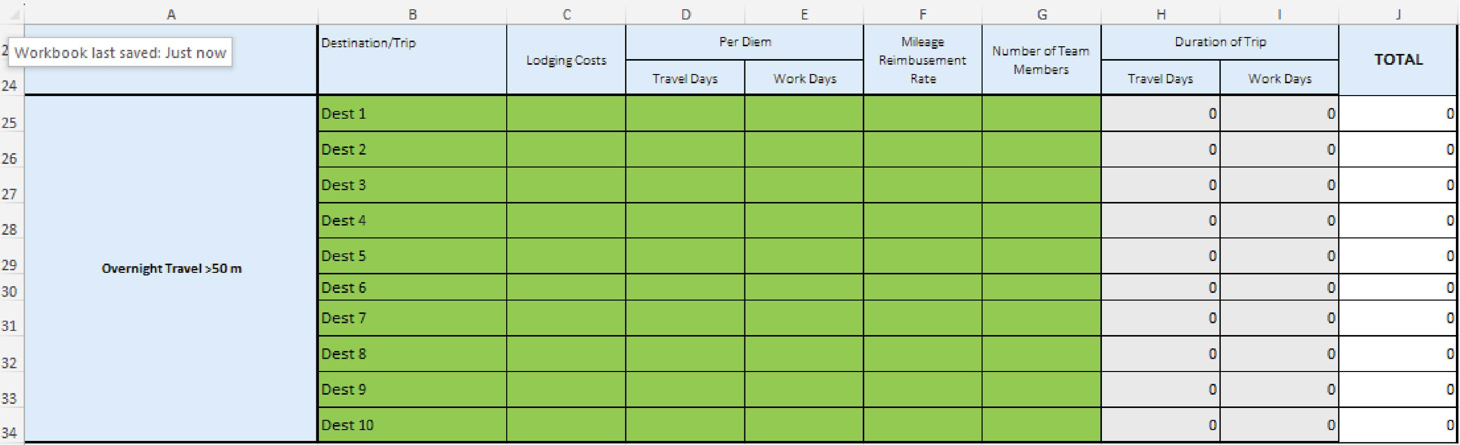
Long Description.
The column headers from columns B through J are destination or trip, lodging costs, per diem with sub-headers travel days and work days, mileage reimbursement rate, number of team members, duration of trip with sub-headers travel days and work days, and total. The entire data-sheet is empty.

Long Description.
The header provided in rows 35 and 41 is the total hours per observer for data collection and the total observers transportation expenses for data, respectively. The data are provided from rows 36 to 39 and from 42 to 44.
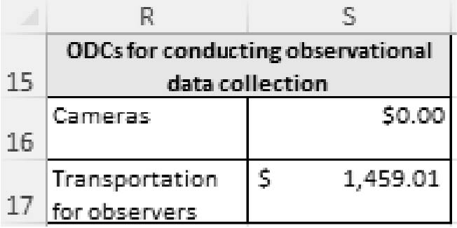
Long Description.
The column header is ODCs for conducting observational data collection. The data are provided in rows 16 and 17.
often risky behaviors occur before, during, and after campaign implementation, researchers can measure shifts in compliance with safe driving practices, helping to determine whether the campaignʼs strategies successfully promote safer road use and reduce risky behaviors.
Step 1: Study Design
To design an observational study, a research and analysis plan must first be developed. Goals, aims, or research questions must be developed and refined, if needed, to assess safety campaign effectiveness. This process must include how data will be collected, what behaviors will be observed, how those behaviors answer each goal or research question, and how that data will be analyzed. At this stage or before, use of video for post hoc analysis or real-time data collection must be determined. Next, the study must be developed where the entire process is drafted and refined to a level where the research plan and protocol can be presented to a safety board, such as an IRB at a university or research institution, or other advisory boards to ensure ethical treatment of participants.
Once approval is given by the appropriate board, further development and testing of the protocol can continue. Refinement can consist of adjusting data-collection metrics by initial behavioral observations made by researchers (like in pilot studies), needs of the project, and other metrics. Once the research team feels the study design is ready for implementation, a pilot study or pilot participants can help further distill the protocol and highlight potential or current problems in data collection before the full-scale study is initiated, helping to save time, money, and frustration later in data collection. It must be noted that changes to the protocol in this process might require reevaluation by a safety board, possibly adding to the required project time.
Observational study data can be gathered in two primary ways for application in the costing tool: through real-time observation, where a researcher directly observes a site live, or via video-based collection, where video footage is recorded at the site. The latter can involve setting up a dedicated camera or utilizing an existing video feed. The user can choose the data-collection
method by selecting the appropriate value from the drop-down list located in Cell B9. If video-based data collection is selected, the user should input the total cost of cameras in Cell N11, and the total number of cameras per site in Cell N12. The user should also indicate how many variables to observe per vehicle in Cell N16, and the expected time to review each variable per vehicle in minutes (Exhibit 6.3). Regardless of the data-collection type, the user should also input the target number of observations in Cell N13, the total number of locations used in Cell N15, and the total number of observers in Cell N18 (Exhibit 6.3). The overall labor costs for study design are presented in Columns A–J, Rows 6–10 of the Observational Study Cost tab (Exhibit 6.7).
Step 2: Planning and Logistics
Once the study design is complete, planning activities, like scouting locations and conducting training, must commence to set up the foundation for successful data collection. Researchers must scout different locations and conduct initial observations to identify any necessary adjustments to the study parameters. Changes in location or time of day might be required based on factors like traffic flow or pedestrian density, which can affect the data. This scouting phase also allows researchers to make real-time adjustments to optimize conditions for the study. Based on what is learned from location scouting, the user should input the expected potential observations per hour (e.g., number of passing vehicles that may exhibit the behavior being examined) in Cell B8 of the on-site observations tab (5A). The user should also estimate the expected eligibility rate for these potential observations (i.e., the percent of vehicles that qualify as a valid observation) in Cell B9 (Exhibit 6.8). It is also expected that due to the potential for multiple potential observations occurring simultaneously, the observer may not record every instance, and thus the expected completion rate should be input to account for the expected completion rate in Cell B13.
During the planning and logistics phase, training sessions are crucial for preparing the researchers who will collect the data. These sessions enable researchers to become familiar with all aspects of data collection, including behaviors to observe and protocol specifics as well as to clarify any questions they might have. Well-prepared researchers, with a solid understanding of the procedures, will face a lower learning curve during actual data collection, enabling them to work efficiently and accurately from the start. The costing tool assumes that the amount of time it will take to train each observer will be approximately 5 hours, and thus Cell F13 in the Observational Study Cost tab (5) multiples the number of observers by 5, with an additional 5 hours for the project supervisor recorded in Cell D13. The expected labor costs for training are recorded in Cell H13 (Exhibit 6.9).
Step 3: Data Collection
Data collection for observational studies generally involves one or more researchers identifying and documenting behavior in specific locations at specific times. For real-time data collection, researchers will manually document behaviors using a variety of methods like pen and paper, counters, or other electronic documentation. If not collected electronically, these behaviors are then transcribed to electronic means for future analysis. Observations should follow the research protocol developed in Step 1.
The total amount of time per observation day can be input in the on-site observations tab (5A) in Cell B21. The total number of days per week at each site is input in Cell B32, and the total number of weeks needed to complete data collection is given in Cell B33 based on the values input by the user (Exhibit 6.10). This value is used to output the total expected labor for data collection in Cell M27 of Exhibit 6.2.

Long Description.
The column headers from A through J are task, blank, project director, project supervisor, project administration, project associate team, data processing team, estimated overall cost, per the overall study, and per other. The data are provided from rows 6 to 10.

Long Description.
The headers provided in rows 4 and 11 are assumptions about observations in column A and its factor in column B, and assumptions about typical observer hours in column A, respectively. The data are provided from rows 5 to 9 and from 12 to 17.
Step 4: Analyze and Report
Analyze
Data analysis for an observational study is typically straightforward as the data usually comprises simple data counts for observed behaviors rather than more complex data such as vehicle kinematics, and precise measurements that may be present in an NDS. There is typically minimal data processing before analysis, allowing data analysis to begin soon after data collection is complete.
Collected data must be analyzed using the appropriate statistical process, such as a chi-squared test or a correlation test to indicate differences in campaign effectiveness over time as specified in the analysis plan. Labor costs for data analysis are calculated based on the target number of total completed observations specified in Cell N13 (Exhibit 6.3).
Report
Reporting data should summarize and highlight the collected data. Formatting and organization can be done in a variety of ways but should ideally state the objectives, give background information, explain the study design, what was collected, what was analyzed, and provide the results and conclusions drawn from the analysis. Conclusions should be directly tied to study objectives, illustrating how the results affect the understanding of campaign effectiveness. Expected labor costs for analyzing, summarizing, and reporting results are shown in Cell M29 of the Observational Study Costs tab (5) (Exhibit 6.2).
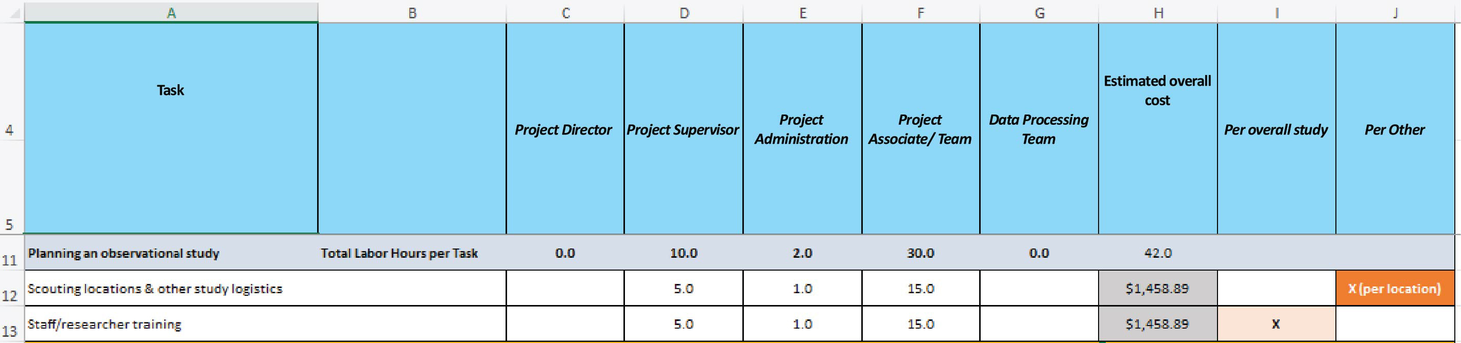
Long Description.
The column headers from A through J are task, blank, project director, project supervisor, project administration, project associate team, data processing team, estimated overall cost, per the overall study, and per other. The header given below is planning an observational study along with its total labor hours per task. The data are provided from rows 11 to 13.

Long Description.
The headers provided in rows 19, 26, and 30 are the number of observations per day, the number days on site needed to meet goal, and the number of weeks in the field needed to meet goal. The data are provided from rows 20 to 24, 27, to 28, and from 31 to 33. Column D shows some notes in rows 20 21, 22, 31, and 32.


