Mercedes Pascual

Center of Marine Biotechnology, University of Maryland Biotechnology Institute

En aquel Imperio, el Arte de la Cartografía logró tal Perfectión que el Mapa de una sola Provincia ocupaba toda una Ciudad, y el Mapa del Imperio, toda una Provincia. Con el tiempo, esos Mapas Desmesurados no satisficieron y los Colegios de Cartógrafos levantaron un Mapa del Imperio, que tenía el tamaño del Imperio y coincidía puntualmente con él. Menos Adictas al Estudio de la Cartografía, las Generaciones Siguientes entendieron que ese dilatado Mapa era Inútil y no sin impiedad lo entregaron a las Inclemencias del Sol y de los Inviernos. . . .

(Suárez Miranda, “Viajes de varones prudentes,” Libro XIV, 1658)

—Jorge Luis Borges y Adolfo Bioy Casares,

“Del Rigor en la Ciencia” en “Cuentos Breves y Extraordinarios.”

In that Empire, the Art of Cartography reached such Perfection that the Map of one Province alone took up the whole of a City, and the Map of the Empire, the whole of a Province. In time, those Unconscionable Maps did not satisfy and the Colleges of Cartographers set up a Map of the Empire which had the size of the Empire itself and coincided with it point by point. Less Addicted to the Study of Cartography, Succeeding Generations understood that this widespread Map was Useless and not without Impiety they abandoned it to the Inclemencies of the Sun and of the Winters . . . .

—Translation from Jorge Luis Borges (1964).

Complexity in ecological systems results not only from a large number of components, but also from nonlinear interactions among the multiple parts. The combined effects of high dimensionality and nonlinearity lead to fundamental challenges in our ability to model, understand, and predict the spatiotemporal dynamics of ecological systems. In this chapter I argue that these challenges are essentially problems of scale—problems arising from the interplay of variability across scales. I address two main consequences of such interplay and sketch avenues for tackling related problems of scale with approaches at the interface of dynamical system theory and time-series analysis.

The first consequence involves a “scale mismatch” between fluctuations of the physical environment and those of ecological variables: In a nonlinear system, forcing at one scale can produce an ecological response with variability at one or more different scales. This scale mismatch challenges our ability to identify key environmental forcings that are responsible for ecological patterns with conventional statistical approaches based on assumptions of linearity.

In the first half of this chapter, theoretical models are used to illustrate the rich array of possible responses to forcing. The models focus on systems for antagonistic interactions, such as those for consumers and their prey or pathogens and their hosts. These examples motivate an important empirical question: How do we identify environmental forcings from ecological patterns without assuming a priori that systems are linear? An alternative approach is proposed, based on novel time-series methods for nonlinear systems. Its general framework should also prove useful to predict ecological responses as a function of environmental forcings. General areas for future application of this approach are outlined in two fields of primary importance to humans—fisheries and epidemiology. In these fields, the role of physical forcings has become the subject of renewed attention, as concern develops for the consequences of human-induced changes in the environment.

The nonlinear models used in the proposed approach are largely phenomenological, allowing for unknown variables and unspecified functional forms. As such, they are best suited for systems whose ecological interactions are well captured by a low number of variables. This brings us to the second part of this chapter, the relationship between scale of description and dynamical properties, including dimensionality.

Here, a second consequence of the interplay of variability across scales is considered, which involves the level of aggregation at which to sample or model ecological systems. This interplay complicates in fundamental ways the problem of aggregation by rendering simple averaging impos-

sible. Aggregation is, however, at the heart of modeling ecological systems—of defining relevant variables to represent their dynamics and of simplifying elaborate models whose high dimensionality precludes understanding and robust prediction.

The second part of this chapter addresses the specific problem of selecting a spatial scale for averaging complex systems. A spatial predator-prey model following the fate of each individual is used to illustrate that fundamental dynamical properties, such as dimensionality and determinism, vary with the spatial scale of averaging. Methods at the interface of dynamical system theory and time-series analysis prove useful to describe this variation and to select, based on it, a spatial scale for averaging. But scale selection is only the first step in model simplification. The problem then shifts to deriving an approximation for the dynamics at the selected scale. The dynamics of the predator-prey system serve to underscore the difficulties that arise when fine-scale spatial structure influences patterns at coarser scales. Open areas for future research are outlined.

Ecologists are well aware of the complicated dynamics that simple, low-dimensional systems can exhibit even in the absence of external forcings. The present challenge is to better understand the dynamics of high-dimensional nonlinear systems and their rich interplay with environmental fluctuations. Here, the perplexing order that nonlinearity creates opens doors to reduce complexity by exploiting relationships between dynamical properties and scale of description. This simplification is important for understanding and predicting dynamics and, ultimately, for better managing human interactions with the environment.

Borges’ “Map of the Empire” gives perhaps a lucid image of attempts to comprehend the dynamics of ecological systems by adding increasing knowledge on their parts. The complexity of such systems leads to fundamental challenges in understanding and predicting their spatiotemporal patterns. Yet ecological systems are essentially dynamic, changing continuously in space and time, and the understanding of this variation is crucial to better understand and manage human interactions with the environment.

Complexity is generally associated with the multiplicity of parts. As such, it is found in a variety of ecological systems. In food webs, for example, the number of trophic categories is large and can rapidly multiply as the observer describes trophic links in greater detail (Abrams et al., 1996). In studies of ecological communities, the large number of species has generated an active debate on the relevant variables and the level of organization at which biodiversity should be defined (Levin and Peale,

1996). The debate is clearly illustrated in the current research on the aggregation of species into functional groups (Dawson and Chapin, 1993; Deutschman, 1996; Rastetter and Shaver, 1995; Solbrig, 1993; Steneck and Dethier, 1994), or in the provocative title “Species as noise in community ecology: Do seaweeds block our view of the kelp forest” (Hay, 1994).

Beyond high dimensionality, however, complex systems possess another defining ingredient, nonlinearity, without which multiple interacting variables would not pose such a formidable challenge. Many ecological rates, such as those associated with per capita population growth, predation, and competition for resources, are not constant but vary as a function of densities. This density dependence in intraspecific and interspecific interactions leads to nonlinearity in ecological systems and in the models we build to capture their dynamics.

Nonlinearity creates a rich array of possible dynamics. Of these, chaos has occupied center stage. First encountered at the turn of this century (Dunhem, 1906; Hadamard, 1898; Poincaré, 1908), chaos raised the unexpected and somewhat disturbing possibility¹ of aperiodic dynamics with sensitivity to initial conditions in deterministic systems. Many decades passed before its definite discovery in the work of Lorenz (1963), Ruelle and Takens (1971), May (1974), and others. A watershed followed in non-linear dynamics research. Hassell et al. (1976) and Schaffer and Kot (1985, 1986) first applied approaches from nonlinear dynamical systems to ecological data; and the debate continues on the relevance of chaos to natural systems (e.g., Ellner and Turchin, 1995; Hastings et al., 1993; Sugihara, 1994). Although chaos remains a fascinating concept, it is on a different and more ubiquitous property of nonlinearity that I wish to focus my attention here, a property of fundamental importance to understanding, predicting, and modeling the dynamics of complex ecological systems.

In nonlinear dynamical systems, variability interacts across scales in space and/or time with consequences far beyond those emphasized so far by ecological studies centered on chaos. Indeed, a main message arising from such studies has been that complicated dynamics are possible in simple, low-dimensional systems, and that highly irregular fluctuations in population numbers can occur in the absence of forcing by environmental fluctuations. Here, I shift the focus to the high-dimensional nature of ecological systems and to their rich interplay with fluctuations of the physical environment.

But how does the interplay of variability across scales matter to ecology? One important consequence of this interplay involves what I call a “scale mismatch” between the fluctuations of the physical environment and those of ecological variables: In a nonlinear system, forcing at one scale can produce an ecological response with variability at one or more different scales. This scale mismatch challenges our ability to identify key

environmental forcings that are responsible for ecological patterns. Indeed, a common approach, implemented with well-known methods such as cross-correlation and cross-spectral analysis, relies on matching scales of variability. This approach concludes that an ecological pattern is caused by a physical factor if their variances share a dominant period or wave-length. Denman and Powell (1984) give numerous examples of successful results with this approach in a review of plankton patterns and physical processes. They point out, however, that as often as not, ecological responses could not be linked to a particular physical scale. One possible explanation is nonlinearity: scale-matching methods should be most successful at establishing cause and effect relationships in linear systems, or close to equilibria, where nonlinear systems are well approximated by linear ones. There is, however, ample evidence for nonlinearity in population growth, ecological interactions, and the response of ecosystems to perturbations (Denman and Powell, 1984; Dwyer and Perez, 1983; Dwyer et al., 1978; Ellner and Turchin, 1995; Turchin and Taylor, 1992).

Another important consequence involves the scale at which to sample or model the dynamics of complex systems and the related problem of aggregating their components in space, time, or level of organization. In nonlinear systems, the interplay of variability across scales complicates in fundamental ways the problem of aggregation by rendering simple averaging impossible (Steele et al., 1993). Aggregation is, however, at the heart of modeling ecological systems—of defining relevant variables to represent and understand their dynamics. Examples include the definition of functional groups in communities (Hay, 1994), trophic levels in food webs (Armstrong, 1994), demographic classes in populations (Caswell and John, 1992), and the density of individuals in spatial systems (Pascual and Levin, 1999b).

To represent the complexities of distributed interactions in fluctuating environments, realistic ecological models increasingly incorporate elements of space, multiple interactions, and stochasticity. However, in the high dimensionality of these models lies both their strength and their weakness: strength because the systems they represent are undoubtedly high dimensional and weakness because one must generally study them by performing large simulations. It is therefore difficult to elucidate the essential processes determining their spatial and temporal dynamics and the critical mechanistic bases of responses to changing environmental conditions. One route to establish such a link is to simplify models to their essentials by aggregating their basic units.

In spatial systems, simplification involves deriving approximations for the dynamics at a coarser spatial scale (Levin and Pacala, 1997). Beyond simplification, this process of scaling dynamics addresses the importance of local detail (Pacala and Deutschman, 1996), the identification

of the scale at which macroscopic descriptions become effectively deterministic (Keeling et al., 1997; Pascual and Levin, 1999b; Rand and Wilson, 1995), and how to represent variability at scales smaller than those that are explicitly included in a model (Steele et al., 1993). These issues pervade the study of complex systems but are especially relevant to ecology where many and perhaps most measurements are taken at smaller scales than those of the patterns of interest.

In summary, problems of scale set fundamental limits to the understanding and prediction of dynamics in complex ecological systems. Below I address the two specific problems of identifying key environmental forcings and selecting a spatial scale for averaging. These are treated, respectively, in the first and second half of the chapter. I propose that methods at the interface of dynamical systems theory and time-series analysis have important applications to problems of scale. Throughout the chapter, connections are drawn to marine systems.

Although biological oceanography has pioneered the concept of scale in ecology (Haury et al., 1978; Steele, 1978), a linear perspective has dominated the view of how environmental and biological scales interact. A few authors have cautioned against simple linearity assumptions (Denman and Powell, 1984; Dwyer and Perez, 1983; Star and Cullen, 1981; Steele, 1988). Here, I further support the need for a nonlinear perspective.

The relations between the two of them must have been fascinating. For things are not what they seem.

—Saul Bellow, It All Adds Up:

From the Dim Past to the Uncertain Future

There is in ecology a long history of dispute between explanations of population and community patterns based on intrinsic biological processes (competition, predator-prey interactions, density dependence, etc.) and explanations based on extrinsic environmental factors (spatial gradients and/or temporal changes in temperature, moisture, light intensity, advection, etc.). In population ecology, Andrewartha and Birch (1954) considered density-independent factors, such as weather, the primary determinants of population abundance. In this view, chance fluctuations played an important role (Birch, 1958). By contrast, Smith (1961) and Nicholson (1958) viewed populations as primarily regulated by density-dependent factors, such as competition, with densities continually tending toward a state of balance in spite of environmental fluctuations (Kingsland, 1985). In community ecology, the concept of interacting spe-

cies as an integrated whole—a superorganism—in which competition leads to a climax stable state (Clements, 1936) contrasted with that of a loose assemblage dominated by stochastic fluctuations (Gleason, 1926). An undercurrent of this debate reemerged with the discovery of chaotic dynamics in the form of the dichotomy “noise versus determinism/’ and it is still detectable today [see, for example, the discussions on the power spectra of population time series (Cohen, 1996; Sugihara, 1996)].

Mathematical approaches to ecological theory were strongly influenced by Clements’ community climax and Nicholson’s population balance (Kingsland, 1985). These ideas found a natural representation in the mathematical concepts of equilibrium and local stability, becoming amenable to analysis within the realm of linear systems. In fact, nonlinear models for density-dependent interactions are well approximated by linear equations, as long as the system lies sufficiently close to equilibrium.

In the past two decades, the concepts of equilibrium and local stability have slowly faded away, with the growing recognition of the dynamic nature of communities and of the full array of possible dynamics in nonlinear models (e.g., May, 1974; Paine and Levin, 1981; Pickett and White, 1985; Schaffer and Kot, 1985). Today, studies of nonlinear systems are also moving away from the simple dichotomy “determinism versus noise” to encompass the interplay of nonlinear ecological interactions with stochasticity (e.g., Ellner and Turchin, 1995; Pascual and Levin, 1999b; Sugihara, 1994). Surprisingly, however, a linear perspective continues to dominate statistical approaches for relating ecological patterns to environmental fluctuations.

I illustrate below, with an array of nonlinear ecological models, the rich potential interplay of intrinsic (biological) processes and the external environment. This interplay limits the ability of conventional time-series methods, such as cross-correlation analysis, to detect environmental forcings that are responsible for population patterns. I outline an alternative approach based on novel time-series methods for nonlinear systems. I end this first half of the chapter with general areas for future application of this approach—fisheries and epidemiology. In these two fields of primary importance to humans, the role of the physical environment has become the subject of renewed attention as concern develops for the consequences of human-induced changes in the environment, particularly in climate.

Ecological models can identify specific conditions leading to scales of variability in population patterns that are different from those in the underlying environment. The following examples center around one com-

mon nonlinear ecological interaction, that between consumers and their resources. The antagonistic interaction between a predator and its prey is well known for its unstable nature leading to oscillatory behavior in the form of persistent cycles or transient fluctuations with slow damping. Such cycles introduce an intrinsic temporal frequency that is capable of interacting with environmental fluctuations.

One well-known example of this interaction is given by predator-prey models under periodic forcing, where one parameter, such as the growth rate of the prey, varies seasonally. These models display a rich array of possible dynamics, including frequency locking, quasi-periodicity, and chaos (Inoue and Kamifukumoto, 1984; Kot et al., 1992; Rinaldi et al., 1993; Schaffer, 1988). In these dynamic regimes, predator and prey can display variability at frequencies other than that of the seasonal forcing. For example, chaotic solutions are aperiodic and exhibit variance at all frequencies.

These predator-prey models have shown that a temporal-scale mismatch can occur when an endogenous and an exogenous cycle interact. Recent work has extended this result to another type of endogenous oscillation, known as generation cycles, which are profoundly different from the prey-escape cycles in predator-prey systems (Pascual and Caswell, 1997a). Generation cycles occur because of interactions between density-dependent processes and population structure—for instance, the population heterogeneity that is due to individual variation in age, size, or developmental stage (deRoos et al., 1992; Nisbet and Gurney, 1985; Pascual and Caswell, 1997a). This individual variation is not accounted for in typical consumer resource models with aggregated variables such as total biomass or density. It introduces high dimensionality in the form of multiple demographic classes or distributed systems (e.g., Tuljapurkar and Caswell, 1996).

Population heterogeneity can play an important role in consumer resource dynamics in variable environments. This was demonstrated with models for the dynamics of a phytoplankton population and a limiting nutrient resource in the experimental system known as the chemostat (Pascual and Caswell, 1997a). The chemostat provides a simple, yet controllable, idealization of an aquatic system with both an inflow and an outflow of nutrients. Most models for phytoplankton ignore population structure and group all cells in a single variable such as total biomass or density. However, a cell does have a life history, the cell division cycle. Each cell progresses through a determinate sequence of events preceding cell division, and the population is distributed in stages of the cell cycle (Figure 1). Models that include population structure (the stages of the cell cycle) can generate oscillatory dynamics under a constant nutrient supply, a behavior that is absent in the corresponding unstructured models

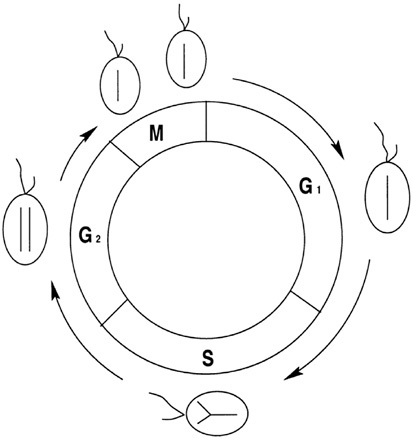
FIGURE 1 The cell cycle. The cell cycle is classically divided into four stages. The cell genome replicates during S, M corresponds to mitosis and cell division, and G1 and G2 denote stages during which most of cell growth takes place. SOURCE: Pascual and Caswell (1997a).

(Pascual, 1994). When forced by a periodic nutrient supply, the models with population structure exhibit aperiodic behavior with variability at temporal scales different from that of the forcing (Figure 2). As a result, the cross correlation between population numbers and nutrient forcing is low for any time lag, and observations of such a system would suggest only a weak link between phytoplankton patterns and nutrient input (Pascual and Caswell, 1997a).

Beyond population structure, another source of high dimensionality in ecological systems is the spatial dimension. Space can fundamentally alter the dynamics of consumer resource systems, as shown with a variety of reaction-diffusion models for interacting populations and random movement (see Okubo, 1980, or Murray, 1989, for a general review). This

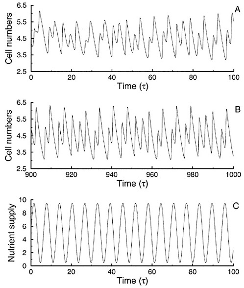
FIGURE 2 Population response to a periodic nutrient forcing. The forcing in the model is the periodic nutrient supply shown in (C). The population response is shown in (A) and (B) for initial and long-term dynamics, respectively. The dynamics of total cell numbers is quasi-periodic and displays variability at frequencies other than that of the forcing. SOURCE: Pascual and Caswell (1997a).

type of model has been used in a biological oceanography to model planktonic systems in turbulent flows. Theoretical studies have focused primarily on the formation of biological patterns in homogeneous environments (Levin and Segel, 1976, 1985). In heterogeneous environments, a biologi-

cal pattern also emerges, which can differ strongly from the underlying spatial forcing (Pascual and Caswell, 1997b). This was shown with a model for a predator and a prey that interact and diffuse along an environmental gradient. Figure 3 shows the resulting irregular spatiotemporal patterns of prey numbers. Weak diffusion on a spatial gradient drives the otherwise periodic predator-prey model into quasi-periodic or chaotic dynamics (Pascual, 1993). In these regimes, the spatial distributions of predator and prey differ from the underlying environmental gradient, with a substantial lack of correlation between population and environmental patterns (Pascual and Caswell, 1997b).

The conditions for a scale mismatch identified by consumer resource models do exist in nature. For example, in the plankton there is evidence for the propensity of predator-prey interactions to oscillate both in the field (McCauley and Murdoch, 1987) and in laboratory experiments (Goulden and Hornig, 1980). There is also evidence for the occurrence of zooplankton generation cycles in the field (deRoos et al., 1992) and for phytoplankton oscillations in chemostat experiments, both transient and persistent, but not accounted for by traditional models without population structure (Caperon, 1969; Droop, 1966; Pickett, 1975; Williams, 1971). The cell cycle provides an explanation for the time delays previously invoked to explain these oscillatory transients (Pascual and Caswell, 1997a).

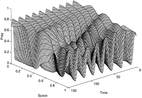
FIGURE 3 Irregular dynamics of prey numbers result from the weak diffusion of prey and predator along an environmental gradient. SOURCE: Pascual (1993).

Above the population level, Dwyer et al. (1978) and Dwyer and Perez (1983) provide compelling evidence for a scale mismatch in plankton dynamics. Their analysis of a 15-year time series showed that phytoplankton abundance in a temperate marine ecosystem displayed variability at multiple harmonics of the seasonal forcing frequency (Dwyer et al., 1978). A series of microcosm experiments, designed to further examine this response, exhibited plankton variability at a number of frequencies, none of which coincided with that of the sinusoidal forcing (Dwyer and Perez, 1983).

I end this series of examples by briefly touching on nonlinear systems with noise. Stochasticity, the extreme manifestation of high dimensionality represents in ecological models not only the unpredictable fluctuations of the environment but also the uncertainty arising from low population numbers. Recent results on the dynamics of epidemiological models give us a glimpse of the unexpected consequences of Stochasticity in nonlinear systems, an area in which surprises are likely to continue and multiply. These models have revealed an elaborate interplay of endogenous cycles with periodic and stochastic forcings (e.g., Engbert and Drepper, 1994; Rand and Wilson, 1991; Sidorowich, 1992). In the models, one parameter, the contact rate, varies seasonally. In the absence of any forcing, the attractor of the system is a limit cycle: The long-term solutions are periodic. With a seasonal contact rate but no Stochasticity, the limit cycle can coexist in phase space with a fascinating structure known as a repellor. Repellors represent the unstable counterparts of the more familiar strange attractors, that is, the geometrical objects in phase space onto which chaotic solutions relax as transients die out. Solutions are attracted toward the stable limit cycle but are continuously pushed away, against the unstable repellor, by the stochastic forcings (Rand and Wilson, 1991). In this way, solutions continuously switch between short-term periodic episodes, determined by the limit cycle, and chaotic transients, revealing the shadow of an unstable invariant set. These transients can be long lasting because trajectories take a long time to escape from the vicinity of the repellor. In addition, because the repellor influences these transients, solutions appear irregular and exhibit variability at a variety of scales different from the periodic forcing.

The above examples raise an important empirical question: How can we identify environmental forcings related to specific population patterns when scales do not match? Furthermore, how do we approach this problem when all the relevant variables are not known and when the time series are short and noisy, two common properties of ecological data?

Recent methods at the interface of dynamical systems and time-series analysis may provide an answer.

I should pause to admit that a scale mismatch will not necessarily occur or be pronounced in all nonlinear systems. Even so, conventional methods might fail to detect relationships between ecological and environmental variables simply because their underlying assumption of linearity is violated. Thus, our main question can be restated in a more general form: How do we identify environmental forcings that are related to specific ecological patterns without assuming a priori that systems are linear?

The basic approach consists of modeling the dynamics of a variable of interest, N(t), such as population density, with a nonlinear equation of the form

(1)

or

(2)

where Tp is a prediction time, f is a nonlinear function, τ is a chosen lag, d is the number of time-delay coordinates, and E_t−τf represents an exogenous variable lagged by τ_f (see below). This basic equation has three key features.

First, the function f is not specified in a rigid form. Instead, the functional form of the model is determined by the data (technically, the model is nonparametric).² This is appealing because we often lack the information to specify exact functional forms.

Second, the model uses time-delay coordinates. This is rooted in a fundamental result from dynamical systems theory, known as “attractor reconstruction” (Takens, 1981), which tackles the problem of not knowing (and therefore not having measured) all the interacting variables of a system. Takens’ theorem essentially tells us that we can use time-delay coordinates as surrogates for the unobserved variables of a system (Figure 4). Although the diagram in Figure 4 considers a simple type of dynamics, the approach extends more generally to complex dynamics. Specifically, if the attractor of the system lies in an n-dimensional space, but one only samples the dynamics of a single variable x_t, then, for almost every time lag τ and for large enough d, the attractor of the d-dimensional time series

(3)

is qualitatively similar to the unknown attractor of the n-dimensional system (Takens, 1981; for an ecological discussion, see Kot et al., 1988). The “embedding dimension” d, which needs to be sufficiently high but not

larger than 2n+1, corresponds to the notion of degrees of freedom, in the sense of providing a sufficient number of variables to specify a point on the attractor (Farmer, 1982).

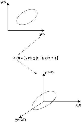
FIGURE 4 Sketch of “attractor reconstruction.” Suppose the system of interest has two variables, x(t) and y(t). If both variables are measured, we can visualize the attractor of the system in phase space by plotting y(t) versus x(t) as a function of time (A). For sufficiently large time, once the effects of initial conditions die out, the resulting trajectory corresponds to the attractor of the system. For periodic dynamics, this attractor is a closed curve known as a limit cycle and is shown in (A). Now suppose that a single variable, x(t), is measured. Then, to “reconstruct” the attractor, a multidimensional time-series is produced in which each coordinate is a lagged value of x(t) [(B), where τ is a fixed lag]. The phase diagram obtained by plotting x(t) versus x(t − τ) versus x(t − 2τ) exhibits an attractor that is topologically equivalent to that of the original system (C).

Third, the model incorporates the effect of an exogenous variable E_t, which influences the dynamics without being altered itself by the state of the system.³ When stochastic, exogenous variables are known as dynamic noise; when deterministic, they can represent trends or periodic patterns. Examples include disturbances such as mortality due to storms, seasonal changes in parameters such as temperature or mixed layer depth, and interannual fluctuations in climate parameters such as those associated with the El Niño Southern Oscillation. The inclusion of an exogenous variable E_t in Equations (1) or (2) is based on an extension by Casdagli (1992) of Takens’ theorem to input-output systems.

Nonlinear (nonparametric) time-series models, such as those in Equations (1) or (2), have been applied recently in ecology to questions on the qualitative type of dynamics of a system and on sensitivity to initial conditions (e.g., Ellner and Turchin, 1995). Beyond these questions, the models have potential but largely unexplored applicability to ecological problems involving environmental variability. Specific applications include (1) identifying the correct frequency of a periodic forcing by distinguishing among different candidate frequencies, (2) identifying environmental forcing(s) by distinguishing among candidate variables for which time series are available, (3) comparing models with and without environmental inputs, and (4) predicting the dynamics of an ecological variable as a function of environmental forcings. Future studies should carefully examine the criteria for model selection, as related not only to accuracy (how well the model fits the data) but also to predictability.

The proposed general framework will apply to systems whose internal dynamics are well captured by a finite and low number of variables (the embedding dimension d). This does not necessarily preclude its application to high-dimensional systems. The attractors of many infinite dimensional dynamical systems are indeed finite dimensional (Farmer, 1982). Moreover, as illustrated in the second part of this chapter, attractor dimension in stochastic nonlinear systems is a function of the scale of description.

A few words of caution. As for correlations, the phenomenological models described here do not necessarily imply causal relationships among variables. They can, however, contribute to the uncovering of such relationships and complement more mechanistic investigations. Here I have argued that incorporating specific information on environmental forcings is a useful yet largely unexplored avenue.

Two areas of ecological research of primary concern to humans—fisheries and epidemiology—appear as good candidates for examining the

usefulness of the above methods. Although seemingly unrelated, they do share some important prerequisites: the availability of data, the presence of nonlinearity in standard dynamical models, and the current interest in environmental effects on their dynamics.

The field of human epidemiology presents some of the best and longest data sets available for ecological research. Not surprisingly, this field has already seen the rich interplay of data analysis and dynamical modeling (e.g., Bolker and Grenfell, 1996; Grenfell and Dobson, 1995; Mollison, 1995; Olsen et al., 1988). Models for the dynamics of human disease are typically variants of a system of differential equations known as SEIR (for the fractions of susceptible, exposed, infectious, and recovered individuals in the host population) (Anderson and May, 1991). SEIR models are nonlinear and display a range of possible dynamics, from limit cycles to chaos (Kot et al., 1988; Schaffer et al., 1990).

For many diseases, the role of the physical environment has become an important current issue (Patz et al., 1996; World Health Organization, 1990), albeit a controversial one in light of climate change and certain speculative predictions (Taubes, 1997). Independent of climate change, however, better knowledge is required on the effects of climate variability. This knowledge can contribute to the implementation of timely preventive measures, particularly in regions of the globe where resources for prevention are either limited or not in place (Bouma and van der Kaay, 1994; Bouma et al., 1994). Climate variability has important manifestations in phenomena such as El Niño and in patterns of rainfall and temperature, which can influence disease dynamics (Bouma et al., 1994; Epstein et al., 1993). An ecological perspective on the dynamics of disease is not completely new. Already present in the first part of the century (Tromp, 1963), this perspective later lost strength, perhaps because medical developments allowed successful intervention, but also because advances in biological research opened the doors to more reductionistic investigations of pathogens and pathogen-host interactions. Today, the increased resistance of pathogens, as well as the breakdown of public health measures in some regions of the globe, argue for complementary research at the environmental level.

Recent studies of one particular human disease related to aquatic environments, cholera, exemplify the growing ecological perspective in infectious disease research (Colwell, 1996). These studies have shown that Vibrio cholerae, the causative agent of epidemic cholera, is a member of the autochthonous microbial flora of brackish water and estuaries (Colwell et al., 1981). Furthermore, experimental work has revealed a relationship between the survival of the bacterium and its attachment to plankton, suggesting a biological reservoir for V. cholerae in nature (Epstein et al., 1993; Huq et al., 1983). The importance of the reservoir and related envi-

ronmental conditions to the patterns of cholera outbreaks remains an area of active research.

The effects of the physical environment are also the subject of renewed attention in fisheries. The International Council for the Exploration of the Sea recently held a symposium on physical-biological interactions in the recruitment dynamics of exploited marine populations in which a major section was devoted to climate variability and recruitment processes. A paper in the recent Special Report by Science on Human-Dominated Ecosystems calls for achieving “better holism” in fisheries management by consideration of broad-scale physical forcing and multiple species (Botsford et al., 1997). As for epidemiology, nonlinearity is present in the standard dynamical models of fisheries, known as stock-recruitment maps (Cushing, 1983). In spite of considerable efforts, prediction with these models has remained a difficult if not elusive goal (Rothschild, 1986).

If this is how things stand, the model of models Mr. Palomar dreams of must serve to achieve transparent models, diaphanous, fine as cobwebs, or perhaps even to dissolve models . . . .

—Italo Calvino, Palomar⁴

Phenomenological models, such as the ones outlined in the first part of this chapter, provide a flexible framework to explore dynamic interactions and to attempt predictions. Ultimately, to better understand the dynamics of a complex system, more mechanistic models must be developed that incorporate the details of known variables and distributed interactions.

In population and community ecology, the extreme implementation of detail is found in models following the fate of each individual. Individual-based models are becoming increasingly popular, in part because technical developments allow us to perform large computer simulations and to sample at increasing resolutions. More importantly, individuals are both a fundamental unit of ecological interaction and a natural scale at which to make measurements, and individual-based models provide a mechanistic foundation that promises a sounder basis for understanding than do purely phenomenological models (Huston et al., 1988; Judson, 1994). Because of their high dimensionality, however, they are extremely sensitive to parameter estimation and prone to error propagation; the potential for analysis is limited, replaced in part by extensive and large simulations (Levin, 1992). It is therefore difficult to understand dynamics and to elucidate critical processes. To address these deficiencies, one is led naturally to issues of aggregation and simplification: When is variability

at the individual level essential to the dynamics of densities? At what spatial scale should densities be defined? How do we derive equations for densities in terms of individual behavior? How does predictability vary as a function of spatial scale? (For examples of recent studies in this area, see Bolker and Pacala, 1997; Levin and Durrett, 1996; Pacala and Deutschman, 1996; Pascual and Levin, 1999a, 1999b). These questions are not limited to the aggregation of individuals, but apply more generally to any basic units on which the local interactions of a model are defined. Indeed, spatial aggregation is also an important problem in landscape and ecosystem models (King, 1992; Levin, 1992; Rastetter et al., 1992; Turner and O’Neill, 1992).

In this second part of the chapter, I address the specific problem of selecting a spatial scale for averaging complex systems. I illustrate with a predator-prey model that fundamental dynamical properties, such as dimensionality and degree of determinism, vary with scale. This variation can be characterized with methods at the interface of dynamical systems and time-series analysis, providing a basis to select a scale for aggregation. But scale selection is only the first step in model simplification. The problem then shifts to deriving an approximation for the dynamics of macroscopic quantities. Here, nonlinearity comes into play by enhancing heterogeneity and allowing fine-scale spatial structure to influence the dynamics at coarser scales.

To address the spatial scale for averaging, I chose a model that provides a useful metaphor for more realistic systems (Durrett and Levin, 2000). Thus, in its “idealized” form, the model already incorporates elements of nonlinearity, stochasticity, and local interactions. It is an individual-based predator-prey system in which the interactions among predators and prey occur in a defined spatial neighborhood. This antagonistic interaction can display a variety of local dynamics, including oscillations and extinctions. Over a landscape, persistence and spatiotemporal patterns reflect the intricate interplay of these local fluctuations. Thus, the model in its qualitative dynamics captures the essence of many other ecological systems, particularly those for host-parasite and host-parasitoid interactions (Comins et al., 1992). The spatial coupling of local fluctuations appears important to the dynamics of epidemics (Grenfell and Harwood, 1997); predators and their prey (Bascompte et al., 1997); and, more generally, of any system whose local feedbacks preclude local equilibria. In the marine environment, an interesting example can be found in benthic systems. In these systems, physical disturbance plays an important role by determining the renewal rate of space, often a limiting re-

source, thereby resetting local species succession. Although disturbance is generally viewed as an external forcing, there is evidence for biological feedbacks affecting its rate. For example, in the rocky intertidal, the barnacle hummocks that form when recruitment is high become unstable and susceptible to removal by wave action (Gaines and Roughgarden, 1985); and the crowding of mussels leads to the disruption of individuals and the formation of focal points for erosion and patch creation (Paine and Levin, 1981). Note that I have so far avoided a precise definition of “local” fluctuations. As illustrated below, the character of fluctuations in nonlinear systems is greatly modified by the spatial scale of sampling.

The predator-prey model follows the fate of individual predators and their prey in continuous time and two-dimensional space. Space consists of a lattice in which each site is either occupied by a predator, occupied by a prey, or empty (Figure 5). The state of a site changes in time according

FIGURE 5 A typical configuration of the predator-prey model. The size of the lattice is 700 × 700. Empty sites are coded in blue, prey sites in red, and predator sites in yellow. Note that the prey forms clusters. These clusters continuously change as they form and disappear through the dynamic interplay of births and deaths. SOURCE: Pascual and Levin (1999b).

to the following processes: Predators hunt for prey by searching within a neighborhood of a prescribed size. Only predators that find prey can reproduce, and they do so at a specified rate. Predators that do not find prey are susceptible to starvation. Prey reproduce locally only if a neighboring site is empty. There is movement through mixing: All neighboring sites exchange state at a constant rate (for details see Durrett and Levin, 2000). In the model, nonlinearity results from predation and birth rates that depend on local densities. Stochasticity is demographic, representing the uncertainty in the fate of any single individual, and is implemented through rates that specify probabilities for the associated events to happen in a given interval of time.⁵

Simulations have shown that the spatiotemporal dynamics of the model perform an intricate dance as clusters or patches form and disappear (Pascual and Levin, 1999b) (Figure 5). As a result, the dynamics of population densities—our macroscopic quantity—change character with the sampling scale (Figure 6): At small size, Stochasticity prevails (panel A); at an intermediate size, the dynamics appear less jagged, more continuous, or smooth (panel B); at a sufficiently large size, small fluctuations around a steady state result from averaging local dynamics that are out of phase (panel C).

A more precise description of these changes is obtained by quantifying how the degree of determinism varies with scale. By definition, the equations of a deterministic model express a causal and therefore predictable relationship between the past and the future: Given exact initial conditions, they completely specify the future state of the system. (Of course, in practice, measurement and dynamical noise are seldom if never absent, limiting predictability in chaotic systems.) When explicit equations are unavailable (as is the case here for densities), the degree of determinism can be evaluated from data through the (short-term) prediction accuracy of a prediction algorithm. The basic steps behind a prediction algorithm are shown in Figure 7. The starting point is by now familiar: Phase-space trajectories are “reconstructed” from a time series of population densities. The local geometry of these trajectories is then used to produce a short-term forecast. In a sense, the algorithm and the associated data constitute an “implicit model” whose (short-term) prediction accuracy reveals the prevalence of determinism versus noise in the dynamics (Kaplan and Glass, 1995).

Prediction accuracy (or predictability) is evaluated by comparing the mean prediction error to the variance of the time series (Kaplan and Glass, 1995) with a quantity such as

(4)

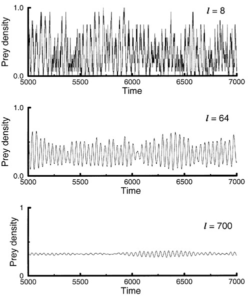
FIGURE 6 Prey densities in windows of different size. Prey densities are computed in a square window of area equal to l². The panels show the temporal behavior of prey density in windows of increasing area: (A), l² = 8 × 8; (B), l² = 64 × 64; (C), l² = 700 × 700. SOURCE: Pascual and Levin (1999b).

If Prediction − r² is close to 0, then the mean prediction error is large with respect to the variance. In this case, the prediction algorithm provides a poor model for the data, and noise is prevalent in the dynamics. If Prediction − r² is close to 1, then the mean prediction error is small; the predic-

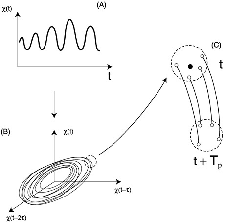
FIGURE 7 The basic steps of a prediction algorithm. From a time series for a single variable, x(t) (in A), phase-space dynamics are reconstructed using time-delay coordinates (in B). For each point on the reconstructed trajectory, a prediction is then obtained as follows: (1) the algorithm chooses a given number k of near neighbors [the open dots in (C) at time t]; (2) the algorithm follows the trajectory of each of these neighbors for the prediction horizon T_p; (3) a forecast is computed from the coordinates of these new points in ways that vary with the specific algorithm (for examples and details see Farmer and Sidorowich, 1987; Kaplan and Glass, 1995; Sauer, 1993; Sugihara and May, 1990). A mean prediction error is computed after repeating these steps for a large number of points.

tion algorithm accounts for a large fraction of the variance, and the dynamics are predominantly deterministic.

Figure 8 shows that determinism increases with spatial scale (Pascual and Levin, 1999b). More interestingly, most of the change in predictability occurs at small scales, and there is little to gain in terms of determinism by considering windows larger than l ≥ 64. At this intermediate scale,

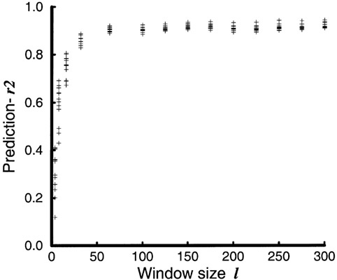
FIGURE 8 Predictability as a function of window size. Not surprisingly, for small window size Prediction − r² is close to 0, indicating the noisy character of the dynamics. At large window size, Prediction − r² is close to 1 because the dynamics of prey numbers are almost constant. Predictability has become high but trivial. More interestingly, the figure reveals the intermediate spatial scale at which high predictability is first achieved. (The basic shape of the curve remains unchanged for different parameters of the prediction algorithm; embedding dimension d = 5, 7, 9, 11; number of neighbors k = d − 2, d, d+2; lag τ = 11; and prediction horizon T_p = τ).

high predictability is achieved with a low number of variables (or number of lags). From the small individual scale to the intermediate scale l_c the dynamics lose their high-dimensional noisy character, with a significant reduction in the number of variables required to specify the state of the system as it changes in time. This reduction is confirmed by estimating the correlation dimension of the attractor (a measure of its dimensionality) (Pascual and Levin, 1999b).⁶

The intermediate scale l_c = 64 provides a natural size at which to model and sample population densities (Keeling et al., 1997; Rand and Wilson, 1995), not only because the dynamics have an important deter-

ministic component, but also because the model would provide information on the predator-prey interaction and its oscillatory nature. Deterministic equations for densities would have to capture the irregular fluctuations of predator and prey. One further, and somewhat unexpected, property of the dynamics at scale l_c underscores that this is not an easy matter. This property is sensitive to initial conditions, the trademark of chaos: Arbitrarily small differences in initial conditions are amplified as trajectories diverge exponentially in phase space (Figure 9).

The significance of sensitivity to initial conditions is not related to chaos per se, but to the problem of deriving equations for population densities. The simpler candidate for such equations would be a “ mean-field” model derived by assuming that space is well mixed and therefore not important. Clearly, such a model, a two-dimensional predator –prey system of differential equations, cannot exhibit sensitivity to initial conditions. For the specific parameters used here, this temporal model exhibits periodic behavior, providing a poor approximation for the dynamics of densities not only at scale l_c but also at larger scales. Thus, a model that ignores spatial detail entirely is inadequate: The dynamics of our macroscopic quantity are affected by the fine-scale spatial clustering.

To better approximate the dynamics of densities at scale l_c, two extensions of simple predator–prey equations come to mind (Pascual and Levin,

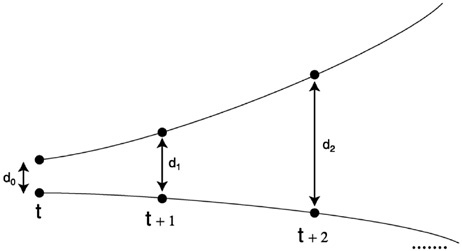
FIGURE 9 Sensitivity to initial conditions. To probe for sensitivity to initial conditions at scale l_c, a time series of prey densities is used to reconstruct the attractor, and the fate of nearby points is examined as follows. For each point, its closest neighbor is found. The distances among the two respective trajectories are recorded as time passes. Pascual and Levin (1999b) show that, on average, the trajectories of nearby points diverge exponentially for small times.

1999b). The first one, of course, consists of incorporating the spatial dimension. Space is likely to be important because l_c falls close to the typical size of the clusters, a scale at which the dynamics of adjacent windows are likely to influence each other in non-negligible ways. There are indeed examples of spatial predator-prey models with chaotic dynamics, such as reaction-diffusion equations in which random movement couples local oscillations (Pascual, 1993; Sherratt et al., 1997). But chaos in these systems requires either specific initial conditions, representing the invasion of prey by predators (Sherratt et al., 1997), or the presence of an environmental gradient (Pascual, 1993). A second but more speculative possibility is that, beyond spatial structure, noise itself—the variability at scales smaller than l_c plays an important role in the dynamics, even at a scale where determinism is prevalent. In this case, deterministic equations that do not incorporate such variability would provide neither a template nor an adequate simplification for the dynamics of densities in window size l_c. These alternatives remain to be explored.

Investigations of scaling in spatial stochastic models for antagonistic interactions, such as the predator-prey system presented here, have only recently been initiated (deRoos et al., 1991; Keeling et al., 1997; Pascual and Levin, 1999b; Rand and Wilson, 1995). Along with results for specific models, these studies will develop general insights and approaches for simplification and scaling in systems with local cycles—systems whose dynamics in a range of spatial scales differ from random fluctuations around an equilibrium. These general results will find application in a variety of ecological systems. Likely candidates are systems that include host–parasite, host–parasitoid, or predator–prey interactions, as well as those where physical disturbance depends on local biological conditions. In the marine environment, predation and physical disturbance play an important role both in the plankton and in the benthos.

In ecology, the application of approaches at the interface of dynamical systems and time-series analysis to problems of aggregation has also only recently begun (Keeling et al., 1997; Little et al., 1996; Pascual and Levin, 1999b). These approaches should be useful for selecting appropriate levels of spatial as well as functional aggregation. Beyond scale selection, however, nonlinear time-series models have also an unexplored potential for the development of empirical methods to scale dynamics.

In the derivation of approximations for dynamics at coarser scales, emphasis so far has been on mathematical approaches (see Levin and Pacala, 1997, for a review). Because such formal derivations may prove impractical if not impossible in many models tailored to specific systems,

there is a need for more empirical methods (e.g., Deutschman, 1996). Here, models that are flexible enough to incorporate what we know, but leave unspecified what we do not know, may prove useful.⁷ For example, we could specify variables and relationships among variables, but not the exact functional form of these relationships.

Finally, we may see the development of methods that take advantage of descriptive scaling laws. Power laws relating a quantity of interest to the scale on which it is measured often describe elaborate patterns in nature (Mandelbrot, 1983; for ecological examples, see Hastings and Sugihara, 1993; Pascual et al., 1995). Such static descriptions, developed in the well-known field of fractals, may also prove useful to the scaling of complex systems in a dynamical context.

I started by presenting nonlinearity and the associated interplay of variability across scales as major roadblocks to the understanding and prediction of dynamics in ecological systems. Somewhat paradoxically, however, nonlinearity itself provides a way around these limitations. As the predator-prey model and other examples in the literature illustrate, nonlinear systems exhibit dynamics with perplexing order. This order, also known as self-organization, is reflected in spatiotemporal patterns that can be described with many fewer variables than those of the original system (Kauffman, 1993). One way to achieve this reduction in complexity is to exploit relationships between scales of description and dynamical properties, including dimensionality and predictability.

At levels of description for which the dynamics of ecological interactions are well captured by low-dimensional systems, we can also hope to better understand and predict responses to environmental forcings, but not without a broader perspective that encompasses nonlinearity.

In the end, in a nonlinear world there are alternatives, both fascinating and open for exploration, to abandoning the “Map of the Empire” to the “Inclemencies of the Sun and of the Winters.”

1. This disturbing character of chaos is illustrated in the title Example of a Mathematical Deduction Forever Unusable (Dunhem, 1906) described in Ruelle (1991).

2. Implementations include feed-forward neural networks or local predictors (for examples see Ellner and Turchin, 1995, or Ellner et al., 1998).

3. E_t can denote a vector time series when multiple forcings or lagged values of a forcing are considered.

4. The original text: ‘Se le cose stanno cosí, il modello dei modelli vagheggiato da Palomar dovrà servire a ottenere dei modelli trasparenti, diafani, sottili come ragnatele; magari addirittura a dissolvere i modelli. . .’ —Italo Calvino, “Palomar.”

5. Specifically, an event occurs at times of a Poisson process with the specified rate.

6. The estimated correlation dimension is 5.6, and the analysis shows that d = 7 is sufficient to reconstruct the attractor (Pascual and Levin, 1999b).

7. An example would be approaches that bring together studies of scaling and inverse methods.

Abrams, P. A., B. A. Menge, G. G. Mittelbach, D. A. Spiller, and P. Yodzis. 1996. The role of indirect effects in food webs. In G. A. Polis and K. O. Winemiller, eds., Food Webs: Integration of Patterns and Dynamics. New York: Chapman & Hall.

Anderson, R. M., and R. M. May. 1991. Infectious Diseases of Humans: Dynamics and Control. Oxford, U.K.: Oxford University Press.

Andrewartha, H. G., and L. C. Birch. 1954. The Distribution and Abundance of Animals. Chicago: University of Chicago Press.

Armstrong, R. A. 1994. Grazing limitation and nutrient limitation in marine ecosystems: Steady-state solutions of an ecosystem model with multiple food chains. Limnology and Oceanography 39(3):597–608.

Bascompte, J., R. V. Solé, and N. Martinez. 1997. Population cycles and spatial patterns in snowshoe hares: An individual-oriented simulation. Journal of Theoretical Biology 187:213–222.

Birch, L. C. 1958. The role of weather in determining the distribution and abundance of animals. Cold Spring Harbor Symposia on Quantitative Biology 22:203–218.

Bolker, B. M., and B. T. Grenfell. 1996. Impact of vaccination on the spatial correlation and dynamics of measles epidemics. Proceedings of the National Academy of Sciences of the United States of America 93:12,648–12,653.

Bolker, B. M., and S. W. Pacala. 1997. Using moment equations to understand stochastically driven spatial pattern formation in ecological systems. Theoretical Population Biology 52:179–197.

Borges, J. L. 1964. Dreamtigers. Austin: University of Texas Press.

Botsford, L. W., J. C. Castilla, and C. H. Peterson. 1997. The management of fisheries and marine ecosystems. Science 277:509–514.

Bouma, M. J, and H. J. van der Kaay. 1994. Epidemic malaria in India and the El Niño Southern Oscillation. Lancet 344:1638–1639.

Bouma, M. J., H. E. Sondorp, and H. J. van der Kaay. 1994. Climate change and periodic epidemic malaria. Lancet 343:1440.

Caperon, J. 1969. Time lag in population growth response in Isochrysis galbana to a variable nitrate environment. Ecology 50(2):188–192.

Casdagli, M. 1992. A dynamical systems approach to modeling input-outputs systems. In M. Casdagli and S. Eubank, eds., Nonlinear Modeling and Forecasting. New York: Addison-Wesley.

Caswell, H., and M. A. John. 1992. From the individual to the population in demographic models. In D. L. DeAngelis and L. J. Gross, eds., Individual-based Models and Approaches in Ecology. Populations, Communities and Ecosystems. New York: Chapman & Hall.

Clements, F. E. 1936. Nature and structure of the climax. Journal of Ecology 24:252–284.

Cohen, J. E. 1996. Unexpected dominance of high frequencies in chaotic nonlinear population models. Nature 378:610–612.

Colwell, R. R. 1996. Global climate and infectious disease: The cholera paradigm. Science 274:2025–2031.

Colwell, R. R., R. J. Seidler, J. Kaper, S. W. Joseph, S. Garges, H. Lockman, D. Maneval, H. Bradford, N. Roberst, E. Remmers, I. Huq, and A. Huq. 1981. Occurrence of Vibrio

cholerae serotype O1 in Maryland and Louisiana estuaries. Applied and Environmental Microbiology 41:555–558.

Comins, H. N., M. P. Hassell, and R. M. May. 1992. The spatial dynamics of host-parasitoid systems. Journal of Animal Ecology 61:735–748.

Cushing, D. H., ed. 1983. Key papers on fish populations. Oxford, U.K.: IRL Press.

Dawson, T. E., and F. S. I. Chapin. 1993. Grouping plants by their form-function characteristics as an avenue for simplification in scaling between leaves and landscapes. In J. R. Ehleringer and C. B. Field, eds., Scaling Physiological Processes: Leaf to Globe. San Diego, Calif.: Academic Press.

Denman, K. L., and T. M. Powell. 1984. Effects of physical processes on planktonic ecosystems in the coastal ocean. Oceanography and Marine Biology Annual Review 22:125–168.

deRoos, A. M., E. McCauley, and W. W. Wilson. 1991. Mobility versus density-limited predator-prey dynamics on different spatial scales. Proceedings of the Royal Society of London Series B 246(1316):117–122.

deRoos, A. M., O. Diekman, and J. A. J. Metz. 1992. Studying the dynamics of structured population models: A versatile technique and its application to Daphnia. American Naturalist 139(1):123–147.

Deutschman, D. H. 1996. Scaling from trees to forests: The problem of relevant detail. Ph.D. Thesis, Cornell University.

Droop, M. R. 1966. Vitamin B₁₂ and marine ecology. III. An experiment with a chemostat. Journal of the Marine Biology Association of the United Kingdom 46:659–671.

Dunhem, P. 1906. La Théorie Physique: Son Objet et sa Structure. Paris: Chevalier et Rivière.

Durrett, R., and S. A. Levin. 2000. Lessons on pattern formation from planet WATOR. Journal of Theoretical Biology.

Dwyer, R. L., and K. T. Perez. 1983. An experimental examination of ecosystem linearization. American Naturalist 121(3):305–323.

Dwyer, R. L., S. W. Nixon, C. A. Oviatt, K. T. Perez, and T. J. Smayda. 1978. Frequency response of a marine ecosystem subjected to time-varying inputs. In J. H. Thorp and J. W. Gibbons, eds., Energy and Environmental Stress in Aquatic Ecosystems. U.S. DOE Symposium Series No. 48 (NTIS No. CONF-771114). Washington, D.C.: U.S. Department of Energy.

Ellner, S. P., and P. Turchin. 1995. Chaos in a ‘noisy’ world: New methods and evidence from time series analysis. American Naturalist 145:343–375.

Ellner, S. P., B. A. Bailey, G. V. Bobashev, A. R. Gallant, B. T. Grenfell, and D. W. Nychka. 1998. Noise and nonlinearity in measles epidemics: Combining mechanistic and statistical approaches to population modeling. American Naturalist 151:425–440.

Engbert, R., and F. R. Drepper. 1994. Qualitative analysis of unpredictability: A case study from childhood epidemics. In J. Grasman and G. van Straten, eds., Predictability and Nonlinear Modeling in Natural Sciences and Economics. Dordrecht, The Netherlands: Kluwer Academic.

Epstein, P. R., T. E. Ford, and R. R. Colwell. 1993. Marine ecosystems. In Health and Climate Change. Lancet 342:1216–1219.

Farmer, J. D. 1982. Chaotic attractors of an infinite-dimensional dynamical system. Physica D 4:366–393.

Farmer, J. D., and J. J. Sidorowich. 1987. Predicting chaotic time series. Physics Review Letters 59:845–848.

Gaines, S., and J. Roughgarden. 1985. Larval settlement rate: A leading determinant of structure in an ecological community of the marine intertidal zone. Proceedings of the National Academy of Sciences of the United States of America 82:3707–3711.

Gleason, H. A. 1926. The individualistic concept of the plant association. Bulletin of the Torrey Botanical Club 53:7–26.

Goulden, C. E., and L. L. Hornig. 1980. Population oscillations and energy reserves in planktonic cladocera and their consequences to competition. Proceedings of the National Academy of Sciences of the United States of America 77:1716–1720.

Grenfell, B. T., and A. P. Dobson. 1995. Ecology of Infectious Diseases in Natural Populations. New York: Cambridge University Press.

Grenfell, B. T., and J. Harwood. 1997. (Meta)population dynamics of infectious diseases. Trends in Ecology and Evolution 12(10):395–399.

Hadamard, J. 1898. Les surfaces à curbures opposées et leurs lignes géodesiques. Journal of Mathematical Analyses and Applications 4:27–73(reprinted in Oeuvres de Jacques Hadamard. 1968. Paris: Centre National de la Recherche Scientifique).

Hassell, M. P., G. H. Lawton, and R. M. May. 1976. Patterns of dynamical behavior in single-species populations. Journal of Animal Ecology 45:471–486.

Hastings, A., C. L. Hom, S. P. Ellner, P. Turchin, and H. C. J. Godfray. 1993. Chaos in ecology: Is mother nature a strange attractor. Annual Review of Ecology and Systematics 24:1–33.

Hastings, H. M., and G. Sugihara. 1993. Fractals: A User’s Guide for the Natural Sciences. New York: Oxford University Press.

Haury, L. R., J. A. McGowan, and P. H. Wiebe. 1978. Patterns and processes in the time-space scales of plankton distribution. In J. H. Steele, ed., Spatial Pattern in Plankton Communities. New York: Plenum.

Hay, M. 1994. Species as noise in community ecology: Do seaweeds block our view of the kelp forest? Trends in Ecology and Evolution 9(11):414–416.

Huq, A., E. B. Small, P. A. West, M. I. Huq, R. Rahman, and R. R. Colwell. 1983. Ecological relationships between Vibrio cholerae and planktonic crustacean copepods. Applied and Environmental Microbiology 45(1):275–283.

Huston, M., D. L. DeAngelis, and W. Post. 1988. New computer models unify ecological theory. Biosciences 38:682–691.

Inoue, M., and H. Kamifukumoto. 1984. Scenarios leading to chaos in a forced Lotka-Volterra model. Progress in Theoretical Physics 71(5):931–937.

Judson, O. P. 1994. The rise of the individual-based model in ecology. Trends in Ecology and Evolution 9(1):9–14.

Kaplan, D., and L. Glass. 1995. Understanding Nonlinear Dynamics. New York: Springer-Verlag.

Kauffman, S. A. 1993. The Origins of Order. Self-organization and Selection in Evolution. New York: Oxford University Press.

Keeling, M. J., I. Mezic, R. J. Hendry, J. McGlade, and D. A. Rand. 1997. Characteristic length scales of spatial models in ecology via fluctuation analysis. Philosophical Transactions of the Royal Society of London Series B 352:1589–1601.

King, A. W. 1992. Translating models across scales in the landscape. In C. G. Jones and J. H. Lawton, eds., Linking Species and Ecosystems. New York: Chapman & Hall.

Kingsland, S. E. 1985. Modeling Nature. Episodes in the History of Population Ecology. Chicago: University of Chicago Press.

Kot, M., W. M. Schaffer, G. L. Truty, D. J. Graser, and L. F. Olsen. 1988. Changing criteria for imposing order. Ecological Modelling 43:75–110.

Kot, M., G. S. Sayler, and T. W. Schultz. 1992. Complex dynamics in a model microbial system. Bulletin of Mathematical Biology 54(4):619–648.

Levin, S. A. 1992. The problem of pattern and scale in ecology. Ecology 73(6):1943–1967.

Levin, S. A., and R. Durrett. 1996. From individuals to epidemics. Philosophical Transactions of the Royal Society of London Series B 351:1615–1621.

Levin, S. A., and S. W. Pacala. 1997. Theories of simplification and scaling in ecological systems. In D. Tilman and P. Kareiva, eds., Spatial Ecology: The Role of Space in Population Dynamics and Interspecific Interactions. Princeton, N.J: Princeton University Press.

Levin, S. A., and M. Peale. 1996. Beyond extinction: Rethinking biodiversity. Bulletin of the Santa Fe Institute (Winter 1995–1996):2–4.

Levin, S., and L. A. Segel. 1976. Hypothesis for origin of planktonic patchiness. Nature 259:659.

Levin, S., and L. A. Segel. 1985. Pattern generation in space and aspect. SIAM Review 27(1):45–67.

Little, S. A., S. P. Ellner, M. Pascual, M. Neubert, D. T. Kaplan, T. Sauer, A. Solow, and H. Caswell. 1996. Detecting nonlinear dynamics in spatio-temporal systems: Examples from ecological models. Physica D 96:321–333.

Lorenz, E. N. 1963. Deterministic nonperiodic flow. Journal of Atmospheric Science 20:130–141.

Mandelbrot, B. B. 1983. The Fractal Geometry of Nature. New York: Freeman.

May, R. 1974. Biological populations with non-overlapping generations: Stable points, stable cycles and chaos. Science 186:645–647.

McCauley, E., and W. W. Murdoch. 1987. Cyclic and stable populations: Plankton as a paradigm. American Naturalist 129:97–121.

Mollison, D., ed. 1995. Epidemic Models: Their Structure and Relation to Data. New York: Cambridge University Press.

Murray, J. D. 1989. Mathematical Biology. New York: Springer-Verlag.

Nicholson, A. J. 1958. Dynamics of insect populations. Annual Review of Entomology 3:107–136.

Nisbet, R. M., and W. S. C. Gurney. 1985. Fluctuation periodicity, generation separation, and the expression of larval competition. Theoretical Population Biology 28:150–180.

Okubo, A. 1980. Diffusion and Ecological Problems: Mathematical Problems. Biomathematics, Vol. 10. New York: Springer-Verlag.

Olsen, L. F., G. L. Truty, and W. M. Schaffer. 1988. Oscillations and chaos in epidemics: A nonlinear dynamic study of six childhood diseases in Copenhagen, Denmark. Theoretical Population Biology 33:344–370.

Pacala, S. W., and D. Deutschman. 1996. Details that matter: The spatial distribution of individual trees maintains forest ecosystem function. Oikos 74:357–365.

Paine, R. T., and S. A. Levin. 1981. Intertidal landscapes: Disturbance and the dynamics of pattern. Ecological Monographs 51 (2):145–178.

Pascual, M. 1993. Diffusion-induced chaos in a spatial predator-prey system. Proceedings of the Royal Society of London Series B 251:1–7.

Pascual, M. 1994. Periodic response to periodic forcing of the Droop equations for phytoplankton growth. Journal of Mathematical Biology 32:743–759.

Pascual, M., and H. Caswell. 1997a. From the cell-cycle to population cycles in phytoplankton-nutrient interactions. Ecology 78(3):897–912.

Pascual, M., and H. Caswell. 1997b. Environmental heterogeneity and biological pattern in a chaotic predator-prey system. Journal of Theoretical Biology 185:1–13.

Pascual, M., and S. A. Levin. 1999a. Spatial scaling in a benthic population model with density-dependent disturbance. Theoretical Population Biology 56:106–122.

Pascual M., and S. A. Levin. 1999b. From individuals to population densities: Searching for the intermediate scale of nontrivial determinism. Ecology 80(7):2225–2236.

Pascual, M., F. A. Ascioti, and H. Caswell. 1995. Intermittency in the plankton: A multifractal analysis of zooplankton biomass variability. Journal of Plankton Research 17(6):1209–1232.

Patz, J. A., P. R. Epstein, T. A. Burke, and J. M. Balbus. 1996. Global climate change and emerging infectious diseases. Journal of the American Medical Association 275(3):217–223.

Pickett, J. M. 1975. Growth of Chlorella in a nitrate-limited chemostat. Plant Physiology 55:223–225.

Pickett, S. T. A., and P. S. White. 1985. The Ecology of Natural Disturbance and Patch Dynamics. Orlando, Fla: Academic Press.

Poincaré, H. 1908. Science et Méthode. Paris: Ernest Flammarion.

Rand, D. A., and H. B. Wilson. 1991. Chaotic stochasticity: A ubiquitous source of unpredictability in epidemics. Proceedings of the Royal Society of London Series B 246:179–184.

Rand, D. A., and H. B. Wilson. 1995. Using spatio-temporal chaos and intermediate-scale determinism to quantify spatially extended ecosystems. Proceedings of the Royal Society of London Series B 259:111–117.

Rastetter, E. B., and G. R. Shaver. 1995. Functional redundance and process aggregation: Linking ecosystems and species. In C. G. Jones and J. H. Lawton, eds., Linking Species and Ecosystems. New York: Chapman & Hall.

Rastetter, E. B., A. W. King, B. J. Cosby, G. M. Hornberger, R. V. O’Neill, and J. E. Hobbie. 1992. Aggregating fine-scale ecological knowledge to model coarser-scale attributes of ecosystems. Ecological Applications 2(1):55–70.

Rinaldi, S., S. Muratori, and Y. Kuznetzov. 1993. Multiple attractors, catastrophes, and chaos in seasonally perturbed predator-prey communities. Bulletin of Mathematical Biology 55:15–36.

Rothschild, B. J. 1986. Dynamics of Marine Fish Populations. Cambridge, Mass.: Harvard University Press.

Ruelle, D., 1991. Chance and Chaos. Princeton, N.J.: Princeton University Press.

Ruelle, D., and F. Takens. 1971. On the nature of turbulence. Communications in Mathematical Physics 20:167–192; 23:343–344.

Sauer, T. 1993. Time series prediction by using delay coordinate embedding. In A. S. Weigend and N. A. Gershenfeld, eds., Time Series Prediction: Forecasting the Future and Understanding the Past. SFI Studies in the Sciences of Complexity, Proceedings Vol. XV. Reading, Mass.: Addison Wesley.

Schaffer, W. M. 1988. Perceiving order in the chaos of nature. In M. S. Boyce, ed., Evolution of Life Histories in Mammals, Theory and Pattern. New Haven, Conn.: Yale University Press.

Schaffer, W. M., and M. Kot. 1985. Do strange attractors govern ecological systems? Bioscience 35:342–350.

Schaffer, W. M., and M. Kot. 1986. Chaos in ecological systems: The coals that Newcastle forgot. Trends in Ecology and Evolution 1:58–63.

Schaffer, W. M., L. F. Olsen, G. L. Truty, and S. L. Fulmer. 1990. The case for chaos in childhood epidemics. In S. Krasner, ed., The Ubiquity of Chaos. Washington, D.C.: American Association for the Advancement of Science.

Sherratt, J. A., B. T. Eagan, and M. A. Lewis. 1997. Oscillations and chaos behind predatorprey invasion: Mathematical artifact or ecological reality? Philosophical Transactions of the Royal Society of London Series B 352:21–38.

Sidorowich, J. J. 1992. Repellors attract attention. Nature 355:584–585.

Smith, F. E. 1961. Density dependence in the Australian thrips. Ecology 42:403–407.

Solbrig, O. T. 1993. Plant traits and adaptive strategies: Their role in ecosystem function. In E. D. Schulze and H. A. Mooney, eds., Biodiversity and Ecosystem Function. Berlin: Springer-Verlag.

Star, J. L., and J. J. Cullen. 1981. Spectral analysis: A caveat. Deep-Sea Research 28A:93–97.

Steele, J. H. 1978. Spatial Pattern in Plankton Communities. New York: Plenum.

Steele, J. H. 1988. Scale selection for biodynamic theories. In B. J. Rothschild, ed., Toward a Theory on Biological-Physical Interactions in the World Ocean. Dordrecht, The Netherlands: Kluwer Academic.

Steele, J. H., S. R. Carpenter, J. E. Cohen, P. K. Dayton, and R. E. Ricklefs. 1993. Comparing terrestrial and marine ecological systems. In S. A. Levin, T. M. Powell, and J. H. Steele, eds., Patch Dynamics. Lecture Notes in Biomathematics 96. New York: Springer-Verlag.

Steneck, R. S., and M. N. Dethier. 1994. A functional group approach to the structure of algal-dominated communities. Oikos 69:476–498.

Sugihara, G. 1994. Nonlinear forecasting for the classification of natural time series. Philosophical Transactions of the Royal Society of London Series A 348:477–495.

Sugihara, G. 1996. Out of the blue. Nature 378:559–560.

Sugihara, G., and R. M. May. 1990. Nonlinear forecasting as a way of distinguishing chaos from measurement error in time series. Nature 344:734–741.

Takens, F. 1981. Detecting strange attractors in turbulence. In D. Rand and L. S. Young, eds., Dynamical Systems and Turbulence, Warwick 1980. Lecture Notes in Mathematics Vol. 898. New York: Springer-Verlag.

Taubes, G. 1997. Apocalypse not. Science 278:1004–1006.

Tromp, S. W. 1963. Medical Biometeorology. Weather, Climate and Living Organisms. Amsterdam: Elsevier.

Tuljapurkar, S., and H. Caswell. 1996. Structured Population Models. New York: Chapman & Hall.

Turchin, P., and A. D. Taylor. 1992. Complex dynamics in ecological time series. Ecology 73:289–305.

Turner, M. G., and R. V. O’Neill. 1992. Exploring aggregation in space and time. In C. G. Jones and J. H. Lawton, eds., Linking Species and Ecosystems. New York: Chapman & Hall.

Williams, F. M. 1971. Dynamics of microbial populations. In B. C. Patten, ed., Systems Analysis and Simulation in Ecology, Vol. 1. New York: Academic Press.

World Health Organization (WHO). 1990. Potential Health Effects of Climatic Change. WHO/PEP/90.10. Geneva: WHO.