Census Data Field Guide for Transportation Applications (2025)
Chapter: 17 Scenario: County Level Employment (Number of Jobs) in the United States

CHAPTER 17
Scenario: County Level Employment (Number of Jobs) in the United States
17.1 Overview
This scenario illustrates the use of County Business Patterns (CBP) data and ACS data to estimate the drivers of employment. The scenario highlights the various census data sources that are available to understand economic drivers in the nation.
17.2 Background
Emily Planner has recently joined Transport Departmentʼs Office of Planning, Environment, and Realty (OPER). Her supervisor tells her that OPER is working to gather data to identify different factors influencing available jobs at different spatial resolutions. Emilyʼs supervisor wants her to collect employment and demographic data at the county level for the entire population of the United States. He asks her to examine the relationship between county-level employment and demographic factors using a linear regression model.
17.3 Analysis
Emily accesses the CBP Datasets page of the Census Bureau website (https://www.census.gov/programs-surveys/cbp/data/datasets.html) and selects 2019 as the year for the CBP (Figure 17.1).
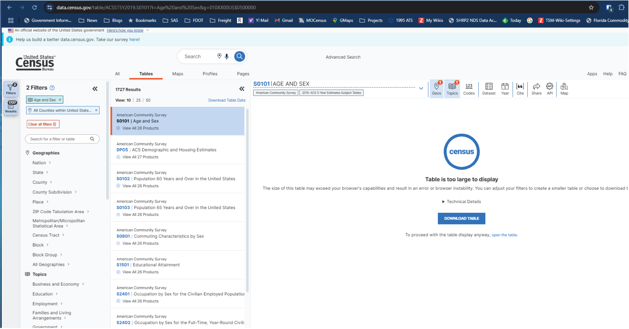
To download the demographic data, Emily navigates to data.census.gov and selects “Advanced Search.” From there, she selects “Age and Sex” as topics, “All Counties within the United States and Puerto Rico” as geography, and “2019” as year to filter the ACS data (Figure 17.2). Then Emily selects Table S0101 for the 5-year data (Figure 17.3).
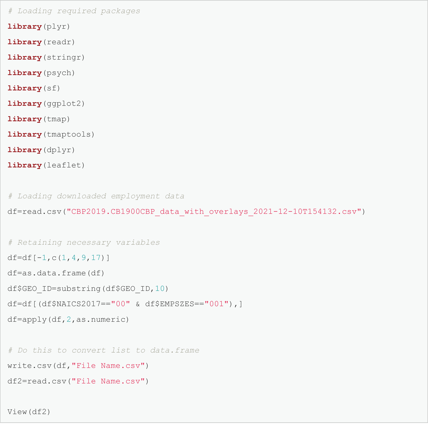
After downloading the CBP and demographic data, Emily uses R to start processing the data to retain only the relevant variables (Figure 17.4). The resulting employment data are shown in Figure 17.5.
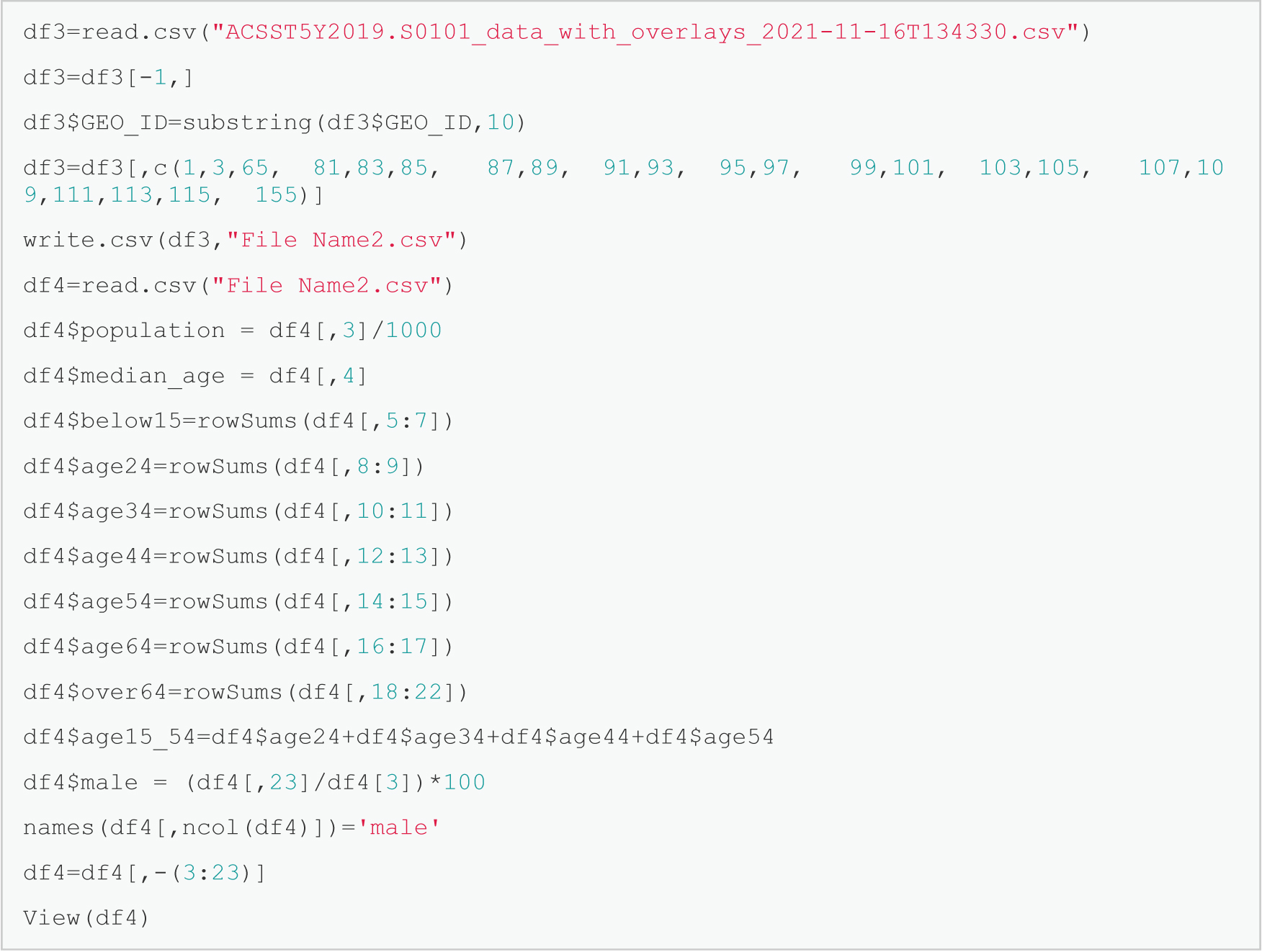
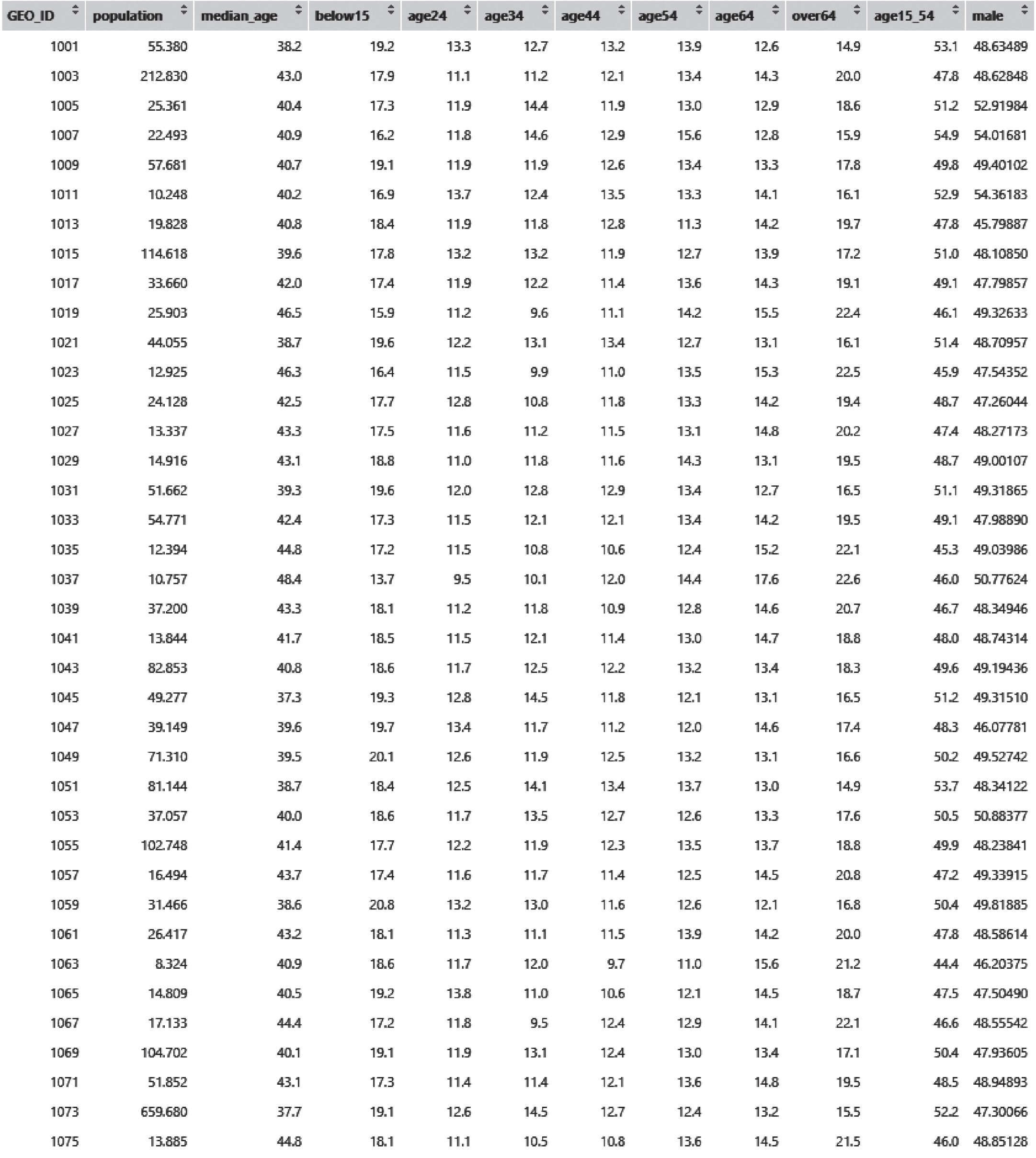
The demographic data are cleaned as well using the process shown in Figure 17.6, and the resulting data table is shown in Figure 17.7.
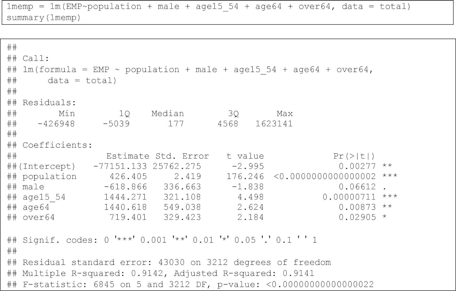
Finally, after merging the employment data and demographic data using GEOIDs, Emily uses the merged dataset to estimate a linear regression model to identify key factors of county-level employment and their impacts. Emily considers several demographic factors such as population, gender distribution, and age distribution for modeling employment. The code for fitting a regression model and the results are shown in Figure 17.8.

Source: U.S. Census Bureau.https://www.census.gov/programs-surveys/cbp/data/datasets.html.
Long Description.
The web page shows the County Business Patterns Datasets from the US Census Bureau website. The heading reads County Business Patterns Datasets. A description explains that CBP datasets are available as comma-separated value files and include data from 1986 to the current year. These datasets provide details such as the number of establishments, employment during the week of March 12, first quarter payroll, and annual payroll, organized by geography, industry, and employment size. The page includes a navigation section on the left with links to API, CBP by Congressional District, CBP Datasets, and CBP Tables. Two dataset entries are visible on the page, titled County Business Patterns 2022 with a release date of June 27, 2024, and County Business Patterns 2020. Each entry is labeled with a Dataset tag. The main navigation bar at the top of the page includes links to Topics, Data and Maps, Surveys and Programs, and Resource Library.
Source: U.S. Census Bureau. https://www.census.gov/programs-surveys/cbp/data/datasets.html.
Long Description.
The U S Census Bureau’s data portal, specifically the American Community Survey, ACS, 5-Year Estimates Subject Tables section. The selected table is S 0 1 0 1 titled Age and Sex. The left panel displays two active filters: Age and Sex, and All Counties within the United States and Puerto Rico. The list below shows search results, including other related tables like D P 0 5, S 0 1 0 2, and S 0 8 0 1. The main panel on the right alerts the user that Table S 0 1 0 1 is too large to display directly in the browser, potentially causing instability. Options are provided to either download the table or open it directly using a separate link. The interface includes tabs for Tables, Maps, Profiles, and Pages, and utility icons for geographies, topics, codes, datasets, years, citation, sharing, API access, and maps. The user is prompted to either reduce the table size with filters or proceed by downloading or opening the full table.

Source: U.S. Census Bureau. https://www.census.gov/programs-surveys/cbp/data/datasets.html.
Long Description.
A pop-up window on the data dot census dot gov platform for selecting vintages of Table S 0 1 0 1 titled Age and Sex from the American Community Survey. The user interface allows choosing between 1-Year and 5-Year Estimates Subject Tables for various years ranging from 2010 to 2023. The 2018 and 2019 vintages of the ACS 5-Year Estimates Subject Tables are selected, and the total compressed download size is indicated as 2.3 MB. A download button labeled Download ZIP is available at the bottom right of the dialog box, allowing the selected dataset files to be downloaded. The main screen in the background shows the active table selection and filters applied, with the data table still too large to display directly in the browser window.
Note: An electronic version of the R code used in the scenarios described in this report is available on the National Academies Press website (nap.nationalacademies.org) in the Resources section of the catalog page for NCHRP Research Report 1108: Census Data Field Guide for Transportation Applications.
Long Description.
# Loading required packages
library(p l y r)
library(read r)
library(string r)
library(psych)
library(s f)
library(g g plot2)
library(t map)
library(t maptools)
library(d p l y r)
library(leaflet)
# Loading downloaded employment data
d f=read.c s v("CBP2019.CB1900CBP_data_with_overlays_2021-12-10T154132.c s v")
# Retaining necessary variables
d f=d f[-1,c(1,4,9,17)]
d f=a s.data.frame(d f)
d f $GEO_ID=substring(d f $GEO_ID,10)
d f=d f[(d f $ N A I C S 2017=="00" & d f $ E M P S Z E S=="001"),]
d f=apply(d f,2,a s.numeric)
# Do this to convert list to data.frame
write.c s v(d f, 'File Name.c s v")
d f 2=read.c s v('File Name.c s v")
View(d f 2)

Long Description.
The table has 4 columns and 35 rows. The column headers include GEO ID, NAICS 2017, EMPSZES, EMP. Row 1: 1001, 0, 1, 11510. Row 2: 1003, 0, 1, 67084. Row 3: 1005, 0, 1, 6893. Row 4: 1007, 0, 1, 3951. Row 5: 1009, 0, 1, 6825. Row 6: 1011, 0, 1, 2061. Row 7: 1013, 0, 1, 6203. Row 8: 1015, 0, 1, 36752. Row 9: 1017, 0, 1, 7118. Row 10: 1019, 0, 1, 4570. Row 11: 1021, 0, 1, 7905. Row 12: 1023, 0, 1, 3006. Row 13: 1025, 0, 1, 6429. Row 14: 1027, 0, 1, 3609. Row 15: 1029, 0, 1, 1669. Row 16: 1031, 0, 1, 13792. Row 17: 1033, 0, 1, 24190. Row 18: 1035, 0, 1, 2679. Row 19: 1037, 0, 1, 1085. Row 20: 1039, 0, 1, 10218. Row 21: 1041, 0, 1, 3117. Row 22: 1043, 0, 1, 25889. Row 23: 1045, 0, 1, 10951. Row 24: 1047, 0, 1, 10030. Row 25: 1049, 0, 1, 18973. Row 26: 1051, 0, 1, 14884. Row 27: 1053, 0, 1, 10006. Row 28: 1055, 0, 1, 30302. Row 29: 1057, 0, 1, 3177. Row 30: 1059, 0, 1, 10718. Row 31: 1061, 0, 1, 3909. Row 32: 1063, 0, 1, 1369. Row 33: 1065, 0, 1, 1906. Row 34: 1067, 0, 1, 3509. Row 35: 1069, 0, 1, 45246.
Note: An electronic version of the R code used in the scenarios described in this report is available on the National Academies Press website (nap.nationalacademies.org) in the Resources section of the catalog page for NCHRP Research Report 1108: Census Data Field Guide for Transportation Applications.
Long Description.
d f 3=read.c s v("ACSST5Y2019.S0101_data_with_overlays_2021-11-16T134330.c s v")
d f 3=d f 3[-1,]
d f 3 $GEO_ID=substring(d f 3 $GEO_ID,10)
d f 3=d f 3[,c(1,3,65, 81,83,85, 87,89, 91,93, 95,97, 99,101, 103,105, 107,109,111,113,115, 155)]
write.c s v(d f 3,"File Name2.c s v")
d f 4=read.c s v("File Name2.csv")
d f 4 $population = d f 4[,3]/1000
d f 4 $median_age = d f 4[,4]
d f 4 $below15=rowSums(d f 4[,5:7])
d f 4 $age24=rowSums(d f 4[,8:9])
d f 4 $age34=rowSums(d f 4[,10:11])
d f 4 $age44=rowSums(d f 4[,12:13])
d f 4 $age54=rowSums(d f 4[,14:15])
d f 4 $age64=rowSums(d f 4[,16:17])
d f 4 $over64=rowSums(d f 4[,18:22])
d f 4 $age15_54=d f 4 $age24+d f 4$age34+d f 4$age44+d f 4$age54
d f 4 $male = (d f 4[,23]/df4[3])*100
names(d f 4[,ncol(d f 4)])='male'
d f 4=d f 4[,-(3:23)]
View(d f 4)
Long Description.
The table has 12 columns and 38 rows. The column headers include GEO ID, population, median age, below 15, age 24, age 34, age 44, age 54, age 64, over 64, age 15 to 54, male. Row 1: 1001, 55.380, 38.2, 19.2, 13.3, 12.7, 13.2, 13.9, 12.6, 14.9, 53.1, 48.63489. Row 2: 1003, 212.830, 43.0, 17.9, 11.1, 11.2, 12.1, 13.4, 14.3, 20.0, 47.8, 48.62848. Row 3: 1005, 25.361, 40.4, 17.3, 11.9, 14.4, 11.9, 13.0, 12.9, 18.6, 51.2, 52.91984. Row 4: 1007, 22.493, 40.9, 16.2, 11.8, 14.6,12.9, 15.6, 12.8, 15.9, 54.9, 54.01681. Row 5: 1009, 57.681, 40.7, 19.1, 11.9, 11.9, 12.6, 13.4, 13.3, 17.8, 49.8, 49.40102. Row 6: 1011, 10.248, 40.2, 16.9, 13.7, 12.4, 13.5, 13.3, 14.1, 16.1, 52.9, 54.36183. Row 7: 1013, 19.828, 40.8, 18.4, 11.9, 11.8, 12.8, 11.3, 14.2, 19.7, 47.8, 45.79887. Row 8: 1015, 114.618, 39.6, 17.8, 13.2, 13.2,11.9, 12.7, 13.9, 17.2, 51.0, 48.10850. Row 9: 1017, 33.660, 42.0, 17.4, 11.9, 12.2, 11.4, 13.6, 14.3, 19.1, 49.1, 47.79857. Row 10: 1019, 25.903, 46.5, 15.9, 11.2, 9.6, 11.1, 14.2, 15.5, 22.4, 46.1, 49.32633. Row 11: 1021, 44.055, 38.7, 19.6, 12.2, 13.1, 13.4, 12.7, 13.1,16.1, 51.4, 48.70957. Row 12: 1023, 12.925, 46.3, 16.4, 11.5, 9.9, 11.0, 13.5, 15.3, 22.5, 45.9, 47.54352. Row 13: 1025, 24.128, 42.5, 17.7, 12.8, 10.8, 11.8, 13.3, 14.2, 19.4, 48.7, 47.26044. Row 14: 1027, 13.337, 43.3, 17.5, 11.6, 11.2, 11.5, 13.1, 14.8, 20.2, 47.4, 48.27173. Row 15: 1029, 14.916, 43.1, 18.8, 11.0, 11.8, 11.6, 14.3, 13.1, 19.5, 48.7, 49.00107. Row 16: 1031, 51.662, 39.3, 19.6, 12.0, 12.8, 12.9, 13.4, 12.7, 16.5, 51.1, 49.31865. Row 17: 1033, 54.771, 42.4, 17.3, 11.5, 12.1, 12.1, 13.4, 14.2, 19.5, 49.1, 47.98890. Row 18: 1035, 12.394, 44.8, 17.2, 11.5, 10.8,10.6,12.4, 15.2, 22.1, 45.3, 49.03986. Row 19: 1037, 10.757, 48.4, 13.7, 9.5, 10.1, 12.0, 14.4, 17.6, 22.6, 46.0, 50.77624. Row 20: 1039, 37.200, 43.3, 18.1, 11.2, 11.8, 10.9, 12.8, 14.6, 20.7, 46.7, 48.34946. Row 21: 1041, 13.844, 41.7, 18.5, 11.5, 12.1, 11.4, 13.0, 14.7, 18.8, 48.0, 48.74314. Row 22 1043, 82.853, 40.8, 18.6, 11.7, 12.5, 12.2, 13.2, 13.4, 18.3, 49.6, 49.19436. Row 23: 1045, 49.277, 37.3, 19.3, 12.8, 14.5, 11.8, 12.1, 13.1, 16.5, 51.2, 49.31510. Row 24:1047, 39.149, 39.6, 19.7, 13.4, 11.7, 11.2, 12.0, 14.6, 17.4, 48.3, 46.07781. Row 25: 1049, 71.310, 39.5, 20.1, 12.6, 11.9, 12.5, 13.2, 13.1, 16.6, 50.2, 49.52742. Row 26: 1051, 81.144, 38.7, 18.4, 12.5, 14.1, 13.4, 13.7, 13.0, 14.9, 53.7, 48.34122. Row 27:1053,37.057, 40.0, 18.6, 11.7, 13.5, 12.7, 12.6, 13.3, 17.6, 50.5, 50.88377. Row 28: 1055,102.748, 41.4, 17.7, 12.2, 11.9, 12.3, 13.5, 13.7, 18.8, 49.9, 48.23841. Row 29: 1057, 16.494, 43.7, 17.4, 11.6, 11.7, 11.4, 12.5, 14.5, 20.8, 47.2, 49.33915. Row 30: 1059, 31.466, 38.6, 20.8, 13.2, 13.0, 11.6, 12.6, 12.1, 16.8, 50.4, 49.81885. Row 31: 1061, 26.417, 43.2, 18.1, 11.3, 11.1, 11.5, 13.9, 14.2, 20.0, 47.8, 48.58614. Row 32: 1063, 8.324, 40.9, 18.6, 11.7, 12.0, 9.7, 11.0, 15.6, 21.2, 44.4, 46.20375. Row 33: 1065, 14.809, 40.5, 19.2, 13.8, 11.0, 10.6, 12.1, 14.5, 18.7, 47.5, 47.50490. Row 34: 1067, 17.133, 44.4, 17.2, 11.8, 9.5, 12.4, 12.9, 14.1, 22.1, 46.6, 48.55542. Row 35: 1069, 104.702, 40.1, 19.1, 11.9, 13.1, 12.4, 13.0, 13.4, 17.1, 50.4, 47.93605. Row 36:1071, 51.852, 43.1, 17.3, 114, 11.4, 12.1, 13.6, 14.8, 19.5, 48.5, 48.94893. Row 37: 1073, 659.680, 37.7, 19.1, 12.6, 14.5, 12.7, 12.4, 13.2, 15.5, 52.2, 47.30066. Row 38: 1075, 13.885, 44.8, 18.1, 11.1, 10.5, 10.8, 13.6, 14.5, 21.5, 46.0, 48.85128.
Long Description.
At the top of the graphic there is a formula:
1m e m p = 1m(EMP~population + male + age15_54 + age64 + over64, data = total)
summary(1m e m p)
Under the heading "Call," there is another formula:
1m(formula = EMP ~ population + male + age15_54 + age64 + over64,
data = total)
Under the heading "Residuals," four categories are shown with values:
Min -426948; 1Q -5039; Median 177; 3Q 4568; Max 1623141
Under the heading "Coefficients," there is material in tabular format with 5 columns and 6 rows. The first column is unnamed, the second column is estimate, the third is standard error, the fourth is t value and the fifth is P r(>|t|). Row details are as follows. Row 1: (Intercept), −77151.133, 25762.275, −2.995, 0.00277 **. Row 2: population, 426.405, 2.419, 176.246, <0.0000000000000002 ***. Row 3: male, −618.866, 336.663, −1.838, 0.06612 .. Row 4: age15_54, 1444.271, 321.108, 4.498, 0.00000711 ***. Row 5: age64, 1440.618, 549.038, 2.624,0.00873 **. Row 6: over64, 719.401, 329.423, 2.184, 0.02905 *.
Following the tabular material is the following:
Signif. codes: 0 ꞌ***ꞌ 0.001 ꞌ**ꞌ 0.01 ꞌ*ꞌ 0.05 ꞌ.ꞌ 0.1 ꞌ ꞌ 1
The final part of the graphic reads:
Residual standard error: 43030 on 3212 degrees of freedom
Multiple R-squared: 0.9142, Adjusted R-squared: 0.9141
F-statistic: 6845 on 5 and 3212 DF, p-value: <0.00000000000000022
Definitions of variable labels in Figure 17.8 are the following:
- EMP = Number of jobs available in the county.
- Population = Population in the county in thousands.
- Male = Percentage of males.
- Age15_54 = Percentage of people between 15 and 54 years old.
- Age64 = Percentage of people between 55 and 64 years old.
- Over64 = Percentage of people older than 64 years.
The model shows that population is a very strong indicator of employment, as expected.
While age effects are statistically significant across all age groups, their significance decreases by half for respondents older than 64 as compared to those who are 15 to 64 years old. Finally, gender was not a statistically significant variable in explaining the number of jobs in a county.


