Census Data Field Guide for Transportation Applications (2025)
Chapter: 16 Scenario: Data Preparation for Travel Demand Model Validation

CHAPTER 16
Scenario: Data Preparation for Travel Demand Model Validation
16.1 Overview
This scenario shows how to use CTPP data for model validation efforts. As with the previous scenarios, it provides R code for a variety of data processing and visualization purposes with the expectation that it will be reproducible.
16.2 Background
Mary Modeler is a recent addition to the staff of a large MPO and has been tasked by her supervisor to compare county-to-county flows from the MPOʼs travel demand model to the CTPP as the first step in validating the model.
16.3 Analysis
Mary accesses the ACTS program website and creates a new selection set showing only counties from the Atlanta Regional Commission and downloads Table A302100—Total Workers (1) (Workers 16 years and over). The resulting dataset is shown in Figure 16.1.
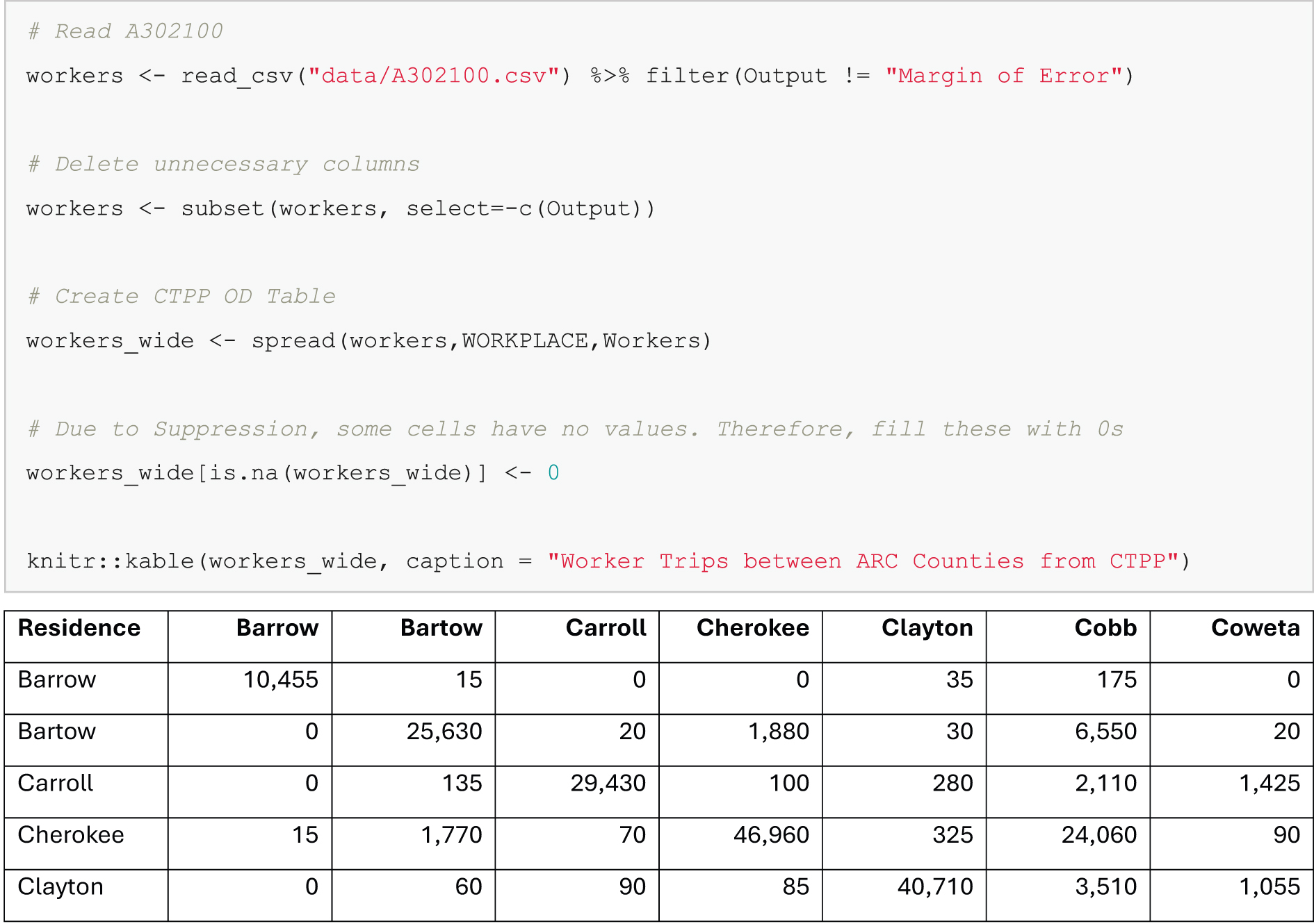
Using R code, she then tweaks the resulting dataset (Figure 16.2) to provide information that will allow her to compare to the MPOʼs travel demand model.
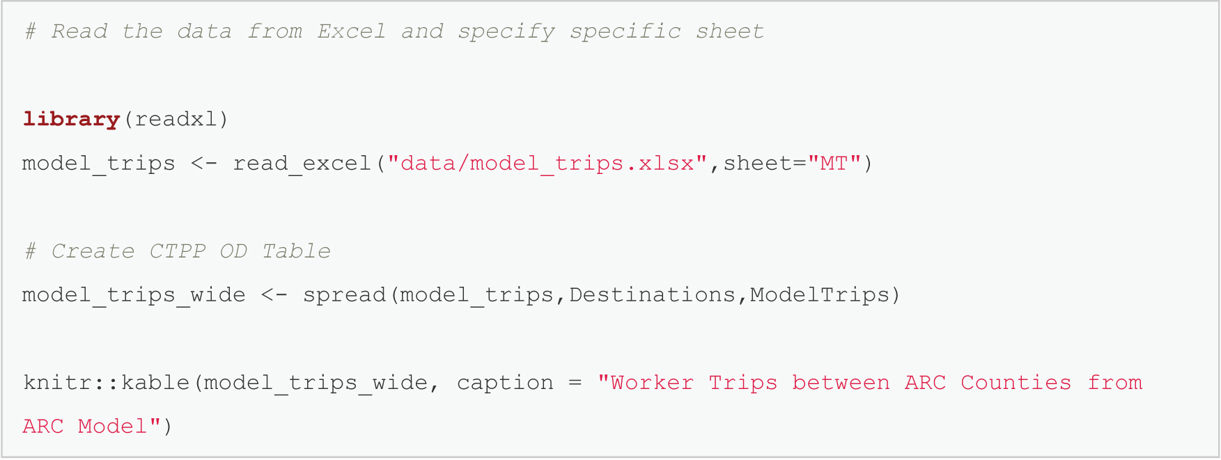
Mary also uses R code to read the model-derived flows (Figure 16.3). The resulting table is shown as Table 16.1.
Finally, before Mary starts validating the model, she produces a chord diagram (Figure 16.4) to compare the differences in county-to-county flows between the MPOʼs travel demand model and the CTPP (Figure 16.5). This information provides her with an understanding of the calibration and validation tweaks she needs to do to match the model flows to the CTPP flows.
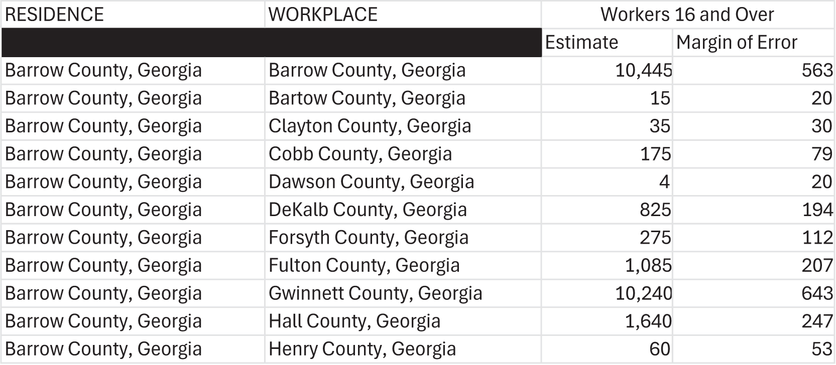
Source: ACTS.
Long Description.
The table has 4 columns and 11 rows. The column headers include Residence, Workplace, Estimated Workers 16 and Over, Margin of Error for Workers 16 and Over. Row 1: Barrow County, Georgia; Barrow County, Georgia; 10,445; 563. Row 2: Barrow County, Georgia; Bartow County, Georgia; 15; 20. Row 3: Barrow County, Georgia; Clayton County, Georgia; 35; 30. Row 4: Barrow County, Georgia; Cobb County, Georgia; 175; 79. Row 5: Barrow County, Georgia; Dawson County, Georgia; 4; 20. Row 6: Barrow County, Georgia; DeKalb County, Georgia; 825; 194. Row 7: Barrow County, Georgia; Forsyth County, Georgia; 275; 112. Row 8: Barrow County, Georgia; Fulton County, Georgia; 1,085; 207. Row 9: Barrow County, Georgia; Gwinnett County, Georgia; 10,240; 643. Row 10: Barrow County, Georgia; Hall County, Georgia; 1,640; 247. Row 11: Barrow County, Georgia; Henry County, Georgia; 60; 53.
Note: An electronic version of the R code used in the scenarios described in this report is available on the National Academies Press website (nap.nationalacademies.org) in the Resources section of the catalog page for NCHRP Research Report 1108: Census Data Field Guide for Transportation Applications.
Long Description.
This graphic shows R code at the top and the resulting table below. The R code reads as follows:
# Read A302100
workers <- read_c s v("data/A302100.c s v") %>% filter(Output != "Margin of Error")
# Delete unnecessary columns
workers <- subset(workers, select=-c(Output))
# Create CTPPOD Table
workers_wide <- spread(workers,WORKPLACE,Workers)
# Due to Suppression, some cells have no values. Therefore, fill these with 0s
workers_wide[i s.n a(workers_wide)] <- 0
k n i t r::kable(workers_wide, caption = "Worker Trips between ARC Counties from CTPP")
The table shown below the R code has 8 columns and 5 rows. The columns are Residence, Barrow, Bartow, Carroll, Cherokee, Clayton, Cobb, and Coweta. Row details are as follows. The table shown below the R code has 8 columns and 5 rows. The columns are Residence, Barrow, Bartow, Carroll, Cherokee, Clayton, Cobb, and Coweta. Row details are as follows. Row 1: Barrow; 10,455; 15; 0; 0; 35; 175; 0. Row 2: Bartow; 0; 25,630; 20; 1,880; 30; 6,550; 20. Row 3: Carroll; 0; 135; 29,430; 100; 280; 2,110; 1,425. Row 4: Cherokee; 15; 1,770; 70; 46,960; 325; 24,060; 90. Row 5: Clayton; 0; 60; 90; 85; 40,710; 3,510; 1,055.
Note: An electronic version of the R code used in the scenarios described in this report is available on the National Academies Press website (nap.nationalacademies.org) in the Resources section of the catalog page for NCHRP Research Report 1108: Census Data Field Guide for Transportation Applications.
Long Description.
# Read the data from Excel and specify specific sheet
library(read x l)
model_trips <- read_excel("data/model_trips.x l s x",sheet="M T")
# Create CTPPOD Table
model_trips_wide <- spread(model_trips,Destinations,ModelTrips)
k n i t r::kable(model_trips_wide, caption = "Worker Trips between ARC Counties from ARC Model")
Source: ACTS.
Long Description.
The table has 9 columns and 21 rows. The column headers include Origins, Barrow, Bartow, Carroll, Cherokee, Clayton, Cobb, Coweta and Dawson. Row 1: Barrow; 13,517; 2; 0; 37; 72; 306; 0; 41. Row 2: Bartow; 0; 28,528; 107; 3,045; 70; 9,968; 2; 14. Row 3: Carroll; 0; 145; 35,803; 50; 499; 2,666; 1,800; 0. Row 4: Cherokee; 24; 2,914; 37; 45,525; 464; 29,158; 4; 356. Row 5: Clayton; 4; 7; 64; 60; 51,278; 4,348; 604; 0. Row 6: Cobb; 18; 3,566; 644; 9,131; 5,923; 229,846; 230; 68. Row 7: Coweta; 0; 4; 2,053; 11; 4,123; 1,800; 33,095; 0. Row 8: Dawson; 17; 25; 0; 512; 3; 290; 0; 4,411. Row 9: DeKalb; 92; 62; 38; 261; 16,696; 15,337; 157; 12. Row 10: Douglas; 1; 196; 2,881; 138; 2,660; 10,853; 916; 0. Row 11: Fayette; 0; 1; 211; 10; 6,908; 1,933; 2,738; 0. Row 12: Forsyth; 222; 151; 0; 3,041; 208; 4,044; 1; 2,502. Row 13: Fulton; 103; 281; 402; 2,711; 25,255; 33,995; 1,321; 190. Row 14: Gwinnett; 4,082; 46; 9; 1,122; 3,959; 10,988; 29; 365. Row 15: Hall; 872; 3; 0; 338; 53; 489; 0; 1,254. Row 16: Henry; 47; 2; 27; 22; 15,855; 2,324; 375; 0. Row 17: Newton; 169; 1; 1; 1; 1,841; 549; 27; 2. Row 18: Paulding; 0; 2,704; 2,918; 1,495; 1,036; 23,944; 309; 1. Row 19: Rockdale; 65; 0; 4; 18; 2,260; 953; 25; 1. Row 20: Spalding; 0; 0; 12; 1; 2,194; 218; 451; 0. Row 21: Walton; 1,772; 0; 0; 24; 483; 370; 1; 8.
Note: An electronic version of the R code used in the scenarios described in this report is available on the National Academies Press website (nap.nationalacademies.org) in the Resources section of the catalog page for NCHRP Research Report 1108: Census Data Field Guide for Transportation Applications.
Long Description.
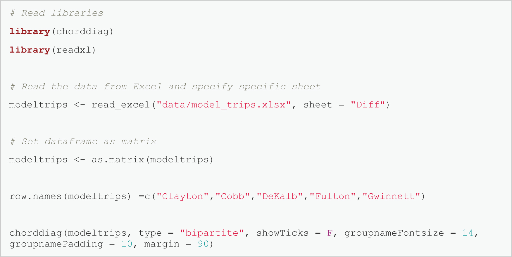
# Read libraries
library(chorddiag)
library(read x l)
# Read the data from Excel and specify specific sheet
modeltrips <- read_excel("data/model_trips.x l s x", sheet = "Diff")
# Set dataframe as matrix
modeltrips <- a s.matrix(modeltrips)
row.names(modeltrips) =c("Clayton","Cobb","DeKalb","Fulton","Gwinnett")
chorddiag(modeltrips, type = "bipartite", showTicks = F, groupnameFontsize = 14, groupnamePadding = 10, margin = 90)
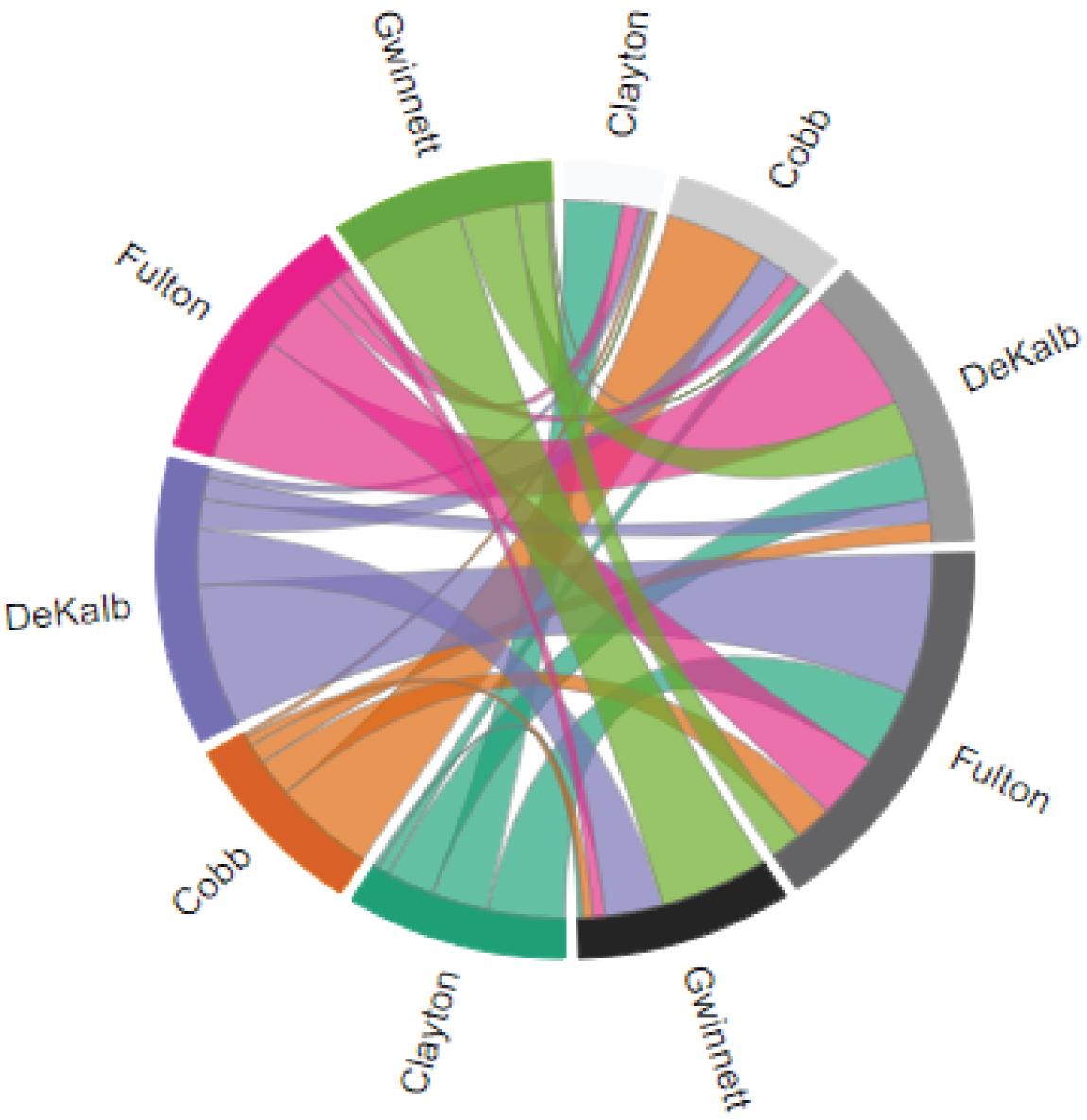
Long Description.
The diagram is a circular chord plot showing differences in trip flows between Clayton, Cobb, DeKalb, Fulton, and Gwinnett counties. Each county is represented twice around the circle, once as an origin and once as a destination. Curved bands connect the counties, representing the magnitude and direction of differences between model-based flows and CTPP data. Thicker bands indicate larger differences. The colors help distinguish counties, and the placement around the circle allows visual comparison of flow mismatches between origin-destination pairs.


