Census Data Field Guide for Transportation Applications (2025)
Chapter: 12 Scenario: Travel Survey Weighting

CHAPTER 12
Scenario: Travel Survey Weighting
12.1 Overview
This scenario, in which CTPP data are used with household survey data to weight a travel survey to represent the population, shows how to weight survey data using a spreadsheet application. Also provided is an understanding of using alternative methods when data are not available. To ensure that the demonstrated analyses are realistic, the fictional region and survey appearing in the scenario are based on actual counties and an actual statewide household survey. A spreadsheet that contains several worksheets related to the weighting of travel survey data in this scenario, can be accessed on the National Academies Press website (nap.nationalacademies.org) by searching for NCHRP Research Report 1108: Census Data Field Guide for Transportation Applications and navigating to “Resources.”
12.2 Background
The Four Seasons Metropolitan Planning Organization (FSMPO) is the transportation planning agency for a mid-sized, four-county region in the center of a Midwestern state. Winter County is the central county with the largest city in the region, a major university, and several large employment centers. Spring County and Summer County are traditional suburban counties, and Autumn County is largely rural.
David, a newly hired transportation planner at FSMPO, had been asked by Donna, the Executive Director, to assemble, process, and analyze available data to support the agencyʼs effort to update its travel demand and to develop a transportation demand profile. David was told that the most recent household travel survey that included the FSMPO region was the state DOT Statewide Travel Survey that was performed in 2016 and 2017. While the survey included more than 11,000 households, the study area was the entire state and only a portion of the survey consisted of FSMPO households. To use the data from the survey, David would need to compare the weighted survey results for the FSMPO households to the CTPP results and re-weight the survey results as needed based on the collected survey data and the census estimates.
Fred, the state DOT household survey manager provided David with the survey data (and documentation), which consisted of the following:
- A household file, with one record per household and variables related to the households, as a whole;
- A person file, with one record per person in the interviewed households and variables at the person level;
- A vehicle file, with one record per vehicle in the surveyed households and vehicle-related variables; and
- A trip file, with one record per reported trip made by the surveyed persons in the surveyed households and data variables related to the trips.
The files were related to each other through common household and person key variables. The household file and person file each contained weighting variables that enable data users to properly expand the survey to statewide and regional control totals based on available census data. The survey weights correct for the deliberate oversampling of some respondent groups that the survey design called for, as well as some of the unexpected biases in the collected data.
Vanessa, the agencyʼs demand modeling manager asked David to begin the analysis by making sure the weighted survey data accurately reflected the regionʼs distribution of households along the variable dimensions commonly used in various components of the travel demand forecasting model. So, David first focused on the household file that Fred provided. (The household file can be accessed via the worksheet called “HHSurvey_State” in the travel survey weighting spreadsheet.)
12.3 Analysis
Davidʼs first step was to filter the household records to only those that pertain to households in the FSMPO region. Of the 11,675 households in the survey database, a total of 1,470 were in the FSMPO region. Winter County had 1,157 households; Summer County had 143 households; Spring County had 92 households; and Autumn County had 78 households.
David obtained the survey codebook and identified the variables in the household file that would be important to compare with census estimates and that could be used for re-weighting the survey data for the FSMPO region. David learned that the household size, workers in the household, and household vehicles variables were very important to Vanessaʼs trip generation and tour generation modeling. In addition, Donna suggested that it would be desirable to analyze the effects of household composition, such as the number of children present in the households and household income, on travel behavior.
David produced pivot tables for these household file variables and then, based on these results, developed recoded versions of several of the variables:
- Actual household sizes were recorded in the survey, so a small number of records had higher numbers of household members. David added a recoded variable that grouped all households with four or more members into a single 4-or-more-person category.
- Similarly, household workers were capped at 3-or-more workers, and household vehicles were capped at 3-or-more vehicles.
- A variable indicating the presence of children in the household (no children, 1 child, 2-or-more children) was created based on the survey fileʼs household size and variables about adults in the household.
- The household income categories were collapsed into a smaller number of categories that matched categories that some CTPP tables use to report income. Because the survey was completed in 2016 and 2017, the income levels reported in the survey were similar on an inflation basis to the year 2016 income levels in the CTPP data, so David did not feel the need to re-calculate the income category limits. This is commonly not the case and often makes the comparison of survey data incomes to CTPP incomes quite difficult.
- David needed to impute missing values in the survey data for the household tenure variable (whether the households own or rent their homes or have other arrangements to be in their homes) and for household income.
To impute missing values, David grouped households based on variables with full information and then randomly matched records with missing variables to other similar households. This
simplified “hot-deck” approach was implemented in a spreadsheet application by producing multivariable pivot tables and then applying the random number generator to select a matching record from which to copy the missing value. (The household file, filtered to the FSMPO region and including the new and recoded variables is shown on the “HHSurvey_FSMPO” worksheet in the travel survey weighting spreadsheet. The new variables are highlighted in yellow.)
David then queried the survey variables of interest using pivot tables. Ideally, David would have liked to perform separate analyses for each of the four counties in the region, but he recognized that the sample sizes of Summer, Spring, and Autumn Counties, individually, were leading to small numbers of records (or zero records) in specific rarer categories. Having few records in specific categories increases the likelihood that weights will be unstable and less reliable. As a result, David decided to conduct his analyses on Winter County as one geographic unit and a second geographic unit made up of the three periphery counties grouped together. This meant there were 1,157 Winter County households and 313 periphery counties households.
David then obtained CTPP data for the two county-level geographic areas (Winter County and the three combined periphery counties). Using the ACTS programʼs web-based data extraction tool, David downloaded several residence-based tables.
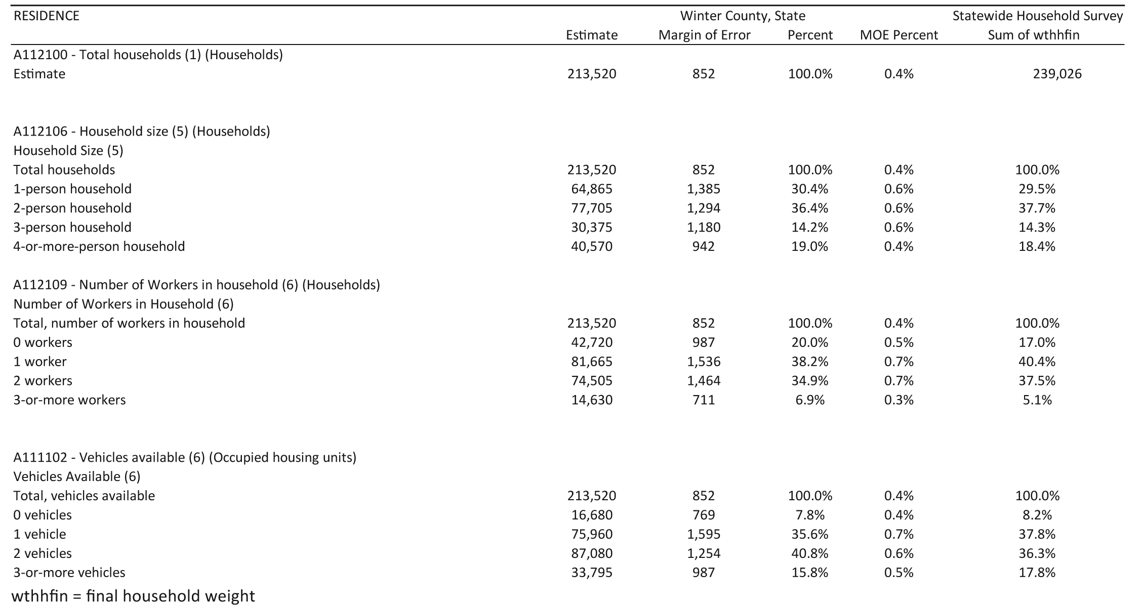
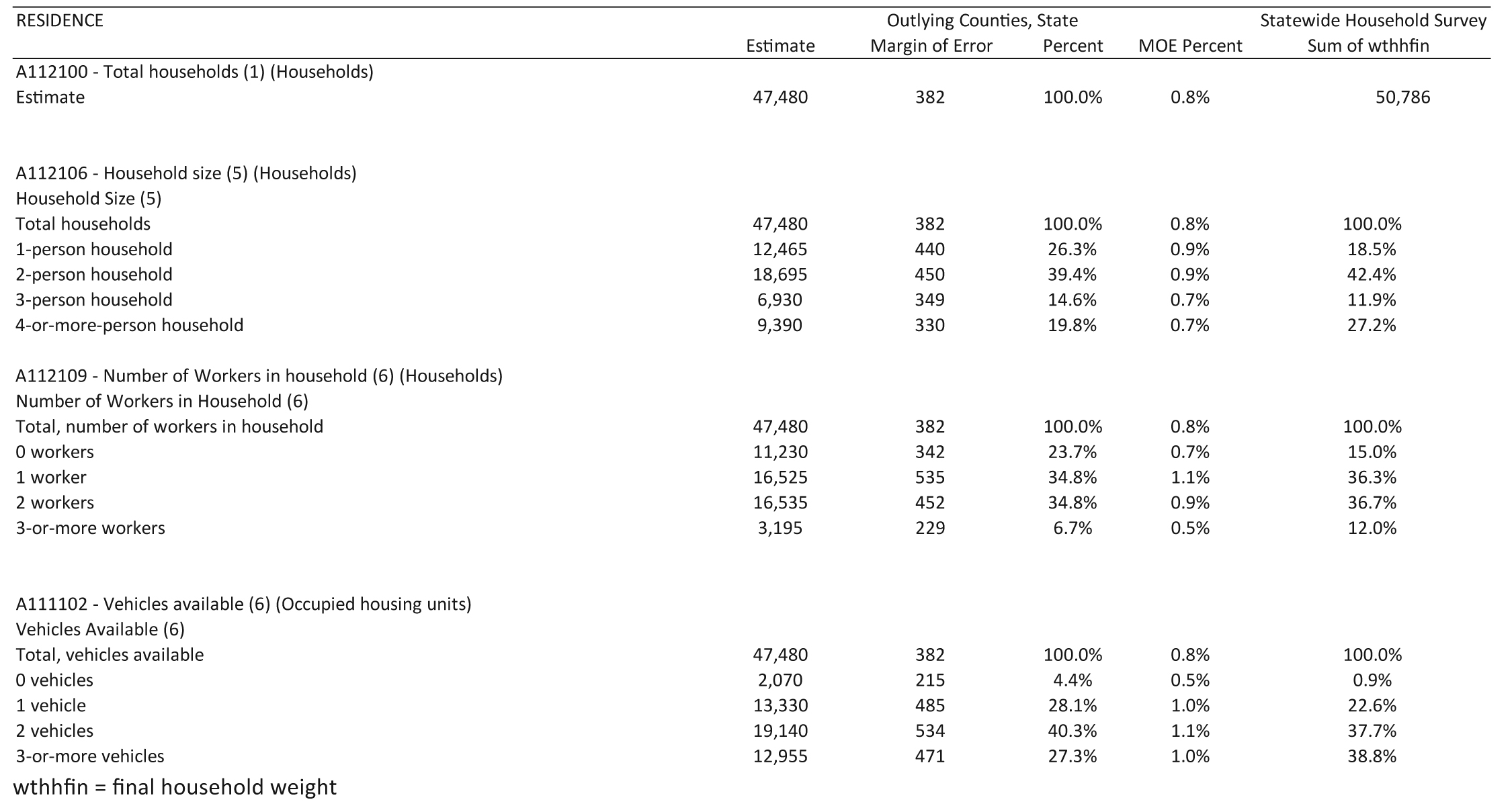
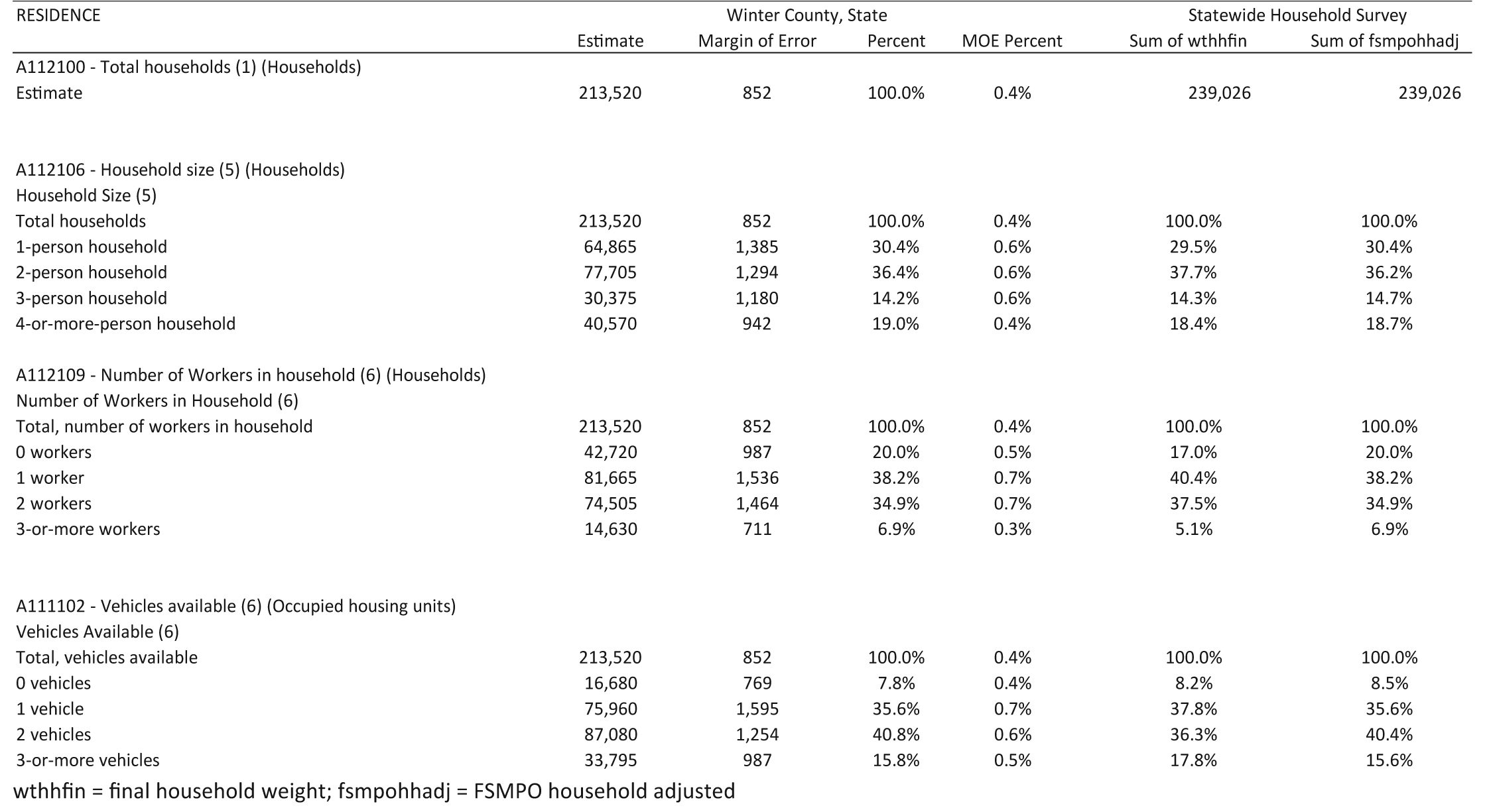
Figure 12.1 and Figure 12.2 compare the CTPP estimates and the weighted survey results for total households, households by household size, households by number of workers, and households by vehicles available for Winter County and the three grouped counties. (The tables shown in Figures 12.1 and 12.2 can also be accessed via the “Comparison” worksheet of the travel survey weighting spreadsheet).
The first thing that David noted was that the overall total number of households differed between the weighted survey results and the CTPP estimates. The CTPP estimate for Winter County is 213,520 households plus or minus 852 households. The weighted sum of households
Long Description.
The table has 6 columns and 16 rows. The first column is titled Residence. Under the heading Winter County, State, are four columns: estimate, margin of error, percent, and margin of error percent. The sixth column, sum of wthh fin (final household weight), is under the heading Statewide Household Survey . Row details are as follows. Rows 1. A112100 Total households 1 Households: Estimate 213,520; Margin of error 852; Percent 100.0; Margin of error percent 0.4; Statewide household survey sum of wthh fin 239,026. Rows 2 through 6 are under the heading A112106 Household size 5 Households; Household size 5. Row 2. Total households: Estimate 213,520; Margin of error 852; Percent 100.0; Margin of error percent 0.4; Statewide household survey sum of wthh fin 100.0 percent. Row 3. 1-person household: Estimate 64,865; Margin of error 1,385; Percent 30.4; Margin of error percent 0.6; Statewide household survey sum of wthh fin 29.5 percent. Row 4. 2-person household: Estimate 77,705; Margin of error 1,294; Percent 36.4; Margin of error percent 0.6; Statewide household survey sum of wthh fin 37.7 percent. Row 5. 3-person household: Estimate 30,375; Margin of error 1,180; Percent 14.2; Margin of error percent 0.6; Statewide household survey sum of wthh fin 14.3 percent. Row 6. 4-or-more person household: Estimate 40,570; Margin of error 942; Percent 19.0; Margin of error percent 0.4; Statewide household survey sum of wthh fin 18.4 percent. Rows 7 through 11 are under the heading of A112109 Number of workers in household 6 Households; Number of workers in household, 6. Row 7. Total, number of workers in household: Estimate 213,520; Margin of error 852; Percent 100.0; Margin of error percent 0.4; Statewide household survey sum of wthh fin 100.0 percent. Row 8. 0 workers: Estimate 42,720; Margin of error 987; Percent 20.0; Margin of error percent 0.5; Statewide household survey sum of wthh fin 17.0 percent. Row 9. 1 worker: Estimate 81,665; Margin of error 1,536; Percent 38.2; Margin of error percent 0.7; Statewide household survey sum of wthh fin 40.4 percent. Row 10. 2 workers: Estimate 74,505; Margin of error 1,464; Percent 34.9; Margin of error percent 0.7; Statewide household survey sum of wthh fin 37.5 percent. Row 11. 3-or-more workers: Estimate 14,630; Margin of error 711; Percent 6.9; Margin of error percent 0.3; Statewide household survey sum of wthh fin 5.1 percent. Rows 12 through 16 are under the heading of A111102 Vehicles available 6 Occupied housing units; Vehicles available 6. Row 12. Total vehicles available: Estimate 213,520; Margin of error 852; Percent 100.0; Margin of error percent 0.4; Statewide household survey sum of wthh fin 100.0 percent. Row 13. 0 vehicles: Estimate 16,860; Margin of error 769; Percent 7.8; Margin of error percent 0.4; Statewide household survey sum of wthh fin 8.2 percent. Row 14. 1 vehicle: Estimate 75,960; Margin of error 1,595; Percent 35.6; Margin of error percent 0.7; Statewide household survey sum of wthh fin 37.8 percent. Row 15. 2 vehicles: Estimate 87,080; Margin of error 1,254; Percent 40.8; Margin of error percent 0.6; Statewide household survey sum of wthh fin 36.3 percent. Row 16. 3-or-more vehicles: Estimate 33,795; Margin of error 987; Percent 15.8; Margin of error percent 0.5; Statewide household survey sum of wthh fin 17.8 percent.
Long Description.
The table has 6 columns and 16 rows. The first column is Residence. Under the heading Outlying Counties, State, there are four columns: Estimate, Margin of error, Percent, and Margin of error percent. The sixth column, sum of wthh fin (final household weight), is under the heading Statewide Household Survey . Row details are as follows. Row 1. A112100 Total households 1 Households; Estimate: Estimate 47,480; Margin of error 382; Percent 100.0; Margin of error percent 0.8; Statewide household survey sum of wthh fin 50,786. Rows 2 through 6 are subcatgories of A112106 Household size 5 Households, Household size 5. Row 2. Total households: Estimate 47,480; Margin of error 382; Percent 100.0; Margin of error percent 0.8; Statewide household survey sum of wthh fin 100.0 percent. Row 3. 1-person household: Estimate 12,465; Margin of error 440; Percent 26.3; Margin of error percent 0.9; Statewide household survey sum of wthh fin 18.5 percent. Row 4. 2-person household: Estimate 18,695; Margin of error 450; Percent 39.4; Margin of error percent 0.9; Statewide household survey sum of wthh fin 42.4 percent. Row 5. 3-person household: Estimate 6,930; Margin of error 349; Percent 14.6; Margin of error percent 0.7; Statewide household survey sum of wthh fin 11.9 percent. Row 6. 4-or-more-person household: Estimate 9,390; Margin of error 330; Percent 19.8; Margin of error percent 0.7; Statewide household survey sum of wthh fin 27.2 percent. Rows 7 through 11 are subcategories of A112109 Number of workers in household 6 Households; Number of workers in household 6. Row 7. Total number of workers in household: Estimate 47,480; Margin of error 382; Percent 100.0; Margin of error percent 0.8; Statewide household surveysum of wthh fin 100.0 percent. Row 8. 0 workers: Estimate 11,230; Margin of error 342; Percent 23.7; Margin of error percent 0.7; Statewide household survey sum of wthh fin 15.0 percent. Row 9. 1 worker: Estimate 16,525; Margin of error 535; Percent 34.8; Margin of error percent 1.1; Statewide household survey sum of wthh fin 36.3 percent. Row 10. 2 workers; Estimate 16,535; Margin of error 452; Percent 34.8; Margin of error percent 0.9; Statewide household survey sum of wthh fin 36.7 percent. Row 11. 3-or-more workers: Estimate 3,195; Margin of error 229; Percent 6.7; Margin of error percent 0.5; Statewide household survey sum of w t h h fin 12.0 percent. Rows 12 through 16 are under the heading of A111102 Vehicles available 6 Occupied housing units; Vehicles available 6. Row 12. Total vehicles available: Estimate 47,480; Margin of error 382; Percent 100.0; Margin of error percent 0.8; Statewide household survey sum of w t h h fin 100.0 percent. Row 13. 0 vehicles: Estimate 2,070; Margin of error 215; Percent 4.4; Margin of error percent 0.5; Statewide household survey sum of w t h h fin 0.9 percent. Row 14. 1 vehicle: Estimate 13,330; Margin of error 485; Percent 28.1; Margin of error percent 1.0; Statewide household survey sum of w t h h fin 22.6 percent. Row 15. 2 vehicles: Estimate 19,140; Margin of error 534; Percent 40.3; Margin of error percent 1.1; Statewide household survey sum of w t h h fin 37.7 percent. Row 16. 3-or-more vehicles: Estimate 12,955; Margin of error 471; Percent 27.3; Margin of error percent 1.0; Statewide household survey sum of wthh fin 38.8 percent.
from the travel survey for Winter County is 239,026 (Figure 12.1). The periphery counties vary in this way as well (47,480 plus or minus 382 versus 50,786) (Figure 12.2). The CTPP household estimates are based on the 2016 population estimates developed by the Census Bureau in 2017 when the 5-year ACS data tables were developed. The travel survey household estimates reflect 2017 census estimates, but they were controlled only at larger regions of the state. They were not controlled at the county level or the MPO region level. David decided he would rather weight the data to the 2016 estimates that CTPP uses, so all the remaining comparisons of survey and census estimates were made using percentages, rather than direct estimates.
On a percentage basis, the estimates of households by household size for Winter County match fairly well between the CTPP data and the survey. One-person households comprise 30.4 percent plus or minus 0.6 percent of total households in CTPP and 29.5 percent in the household survey. Two-person households are 36.4 percent plus or minus 0.6 percent in the CTPP and 37.7 percent in the survey. Three-person households are 14.2 percent plus or minus 0.6 percent versus 14.3 percent. Four-or-more person households are 19.0 percent plus or minus 0.4 percent versus 18.4 percent. For Winter County, the categories of number of workers in household and vehicles available vary slightly more between the CTPP data and the survey than the household size categories but are still reasonably similar.
The comparisons for the combined periphery counties are not as good as they are for Winter County. For instance, while the CTPP estimates indicate that 19.8 percent plus or minus 0.7 percent of households have four or more people, the survey estimates that 27.2 percent of households are this size. More significant differences like this one can be seen in the estimates for number of workers in household and vehicles available.
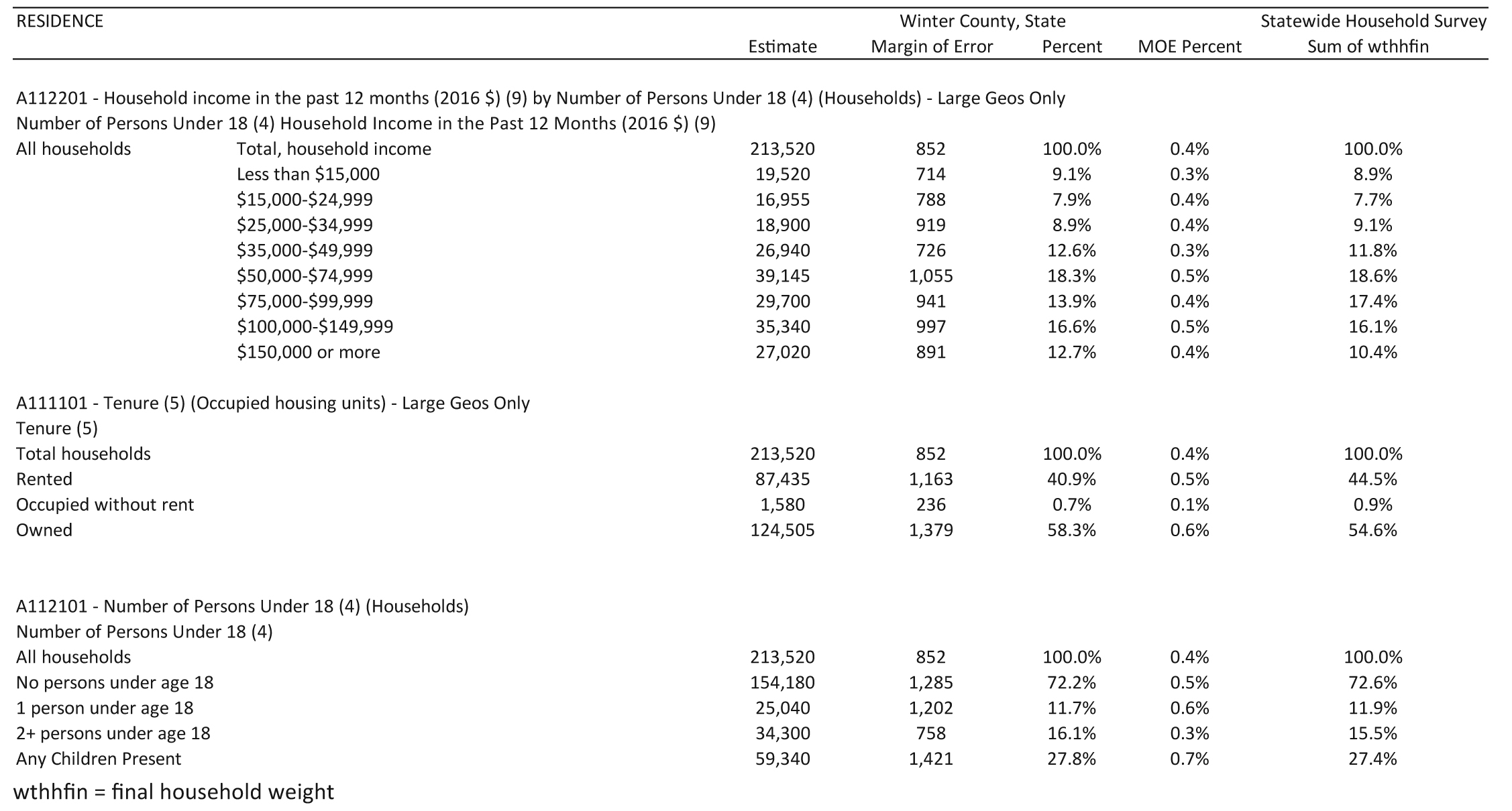
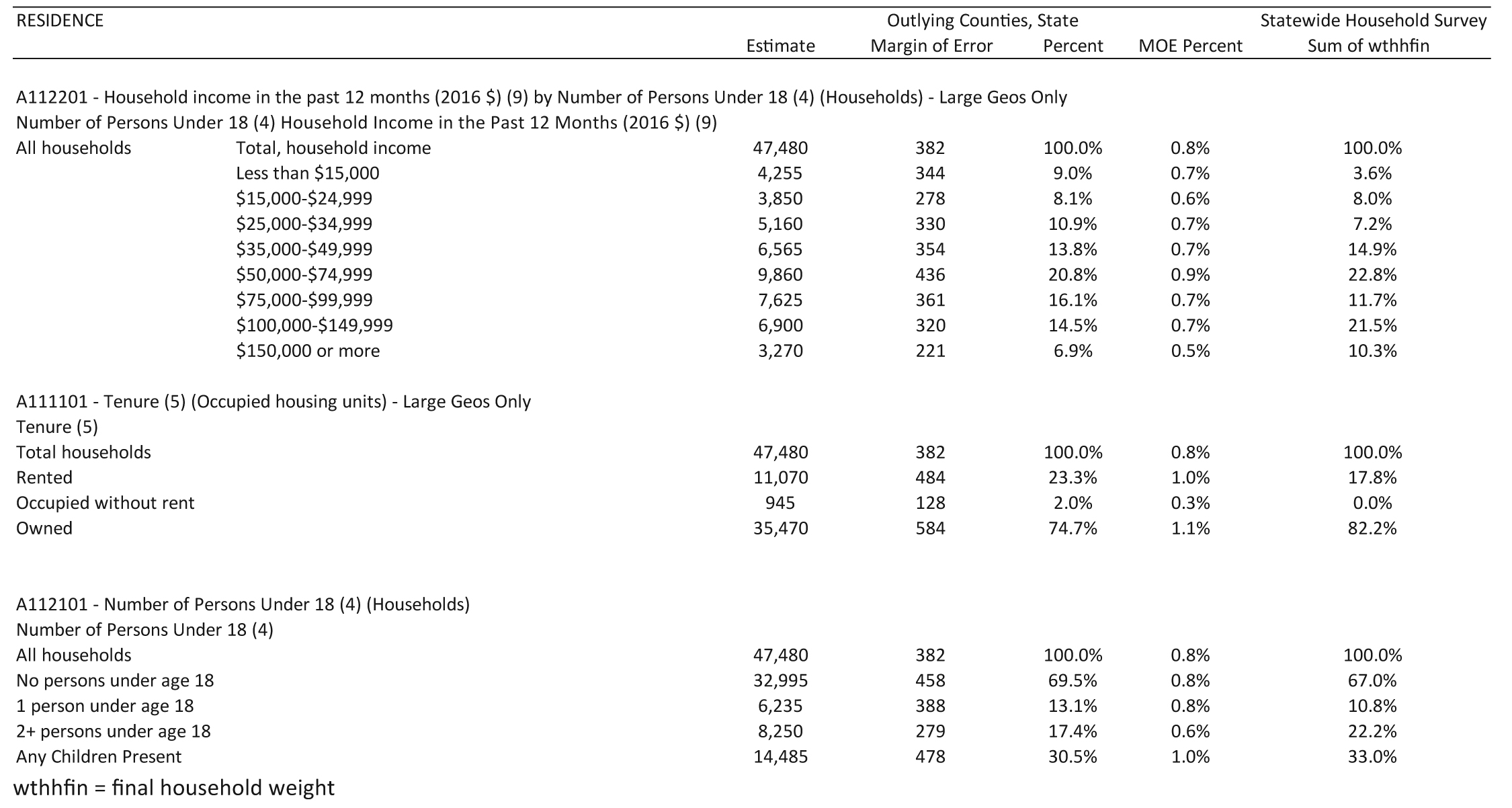
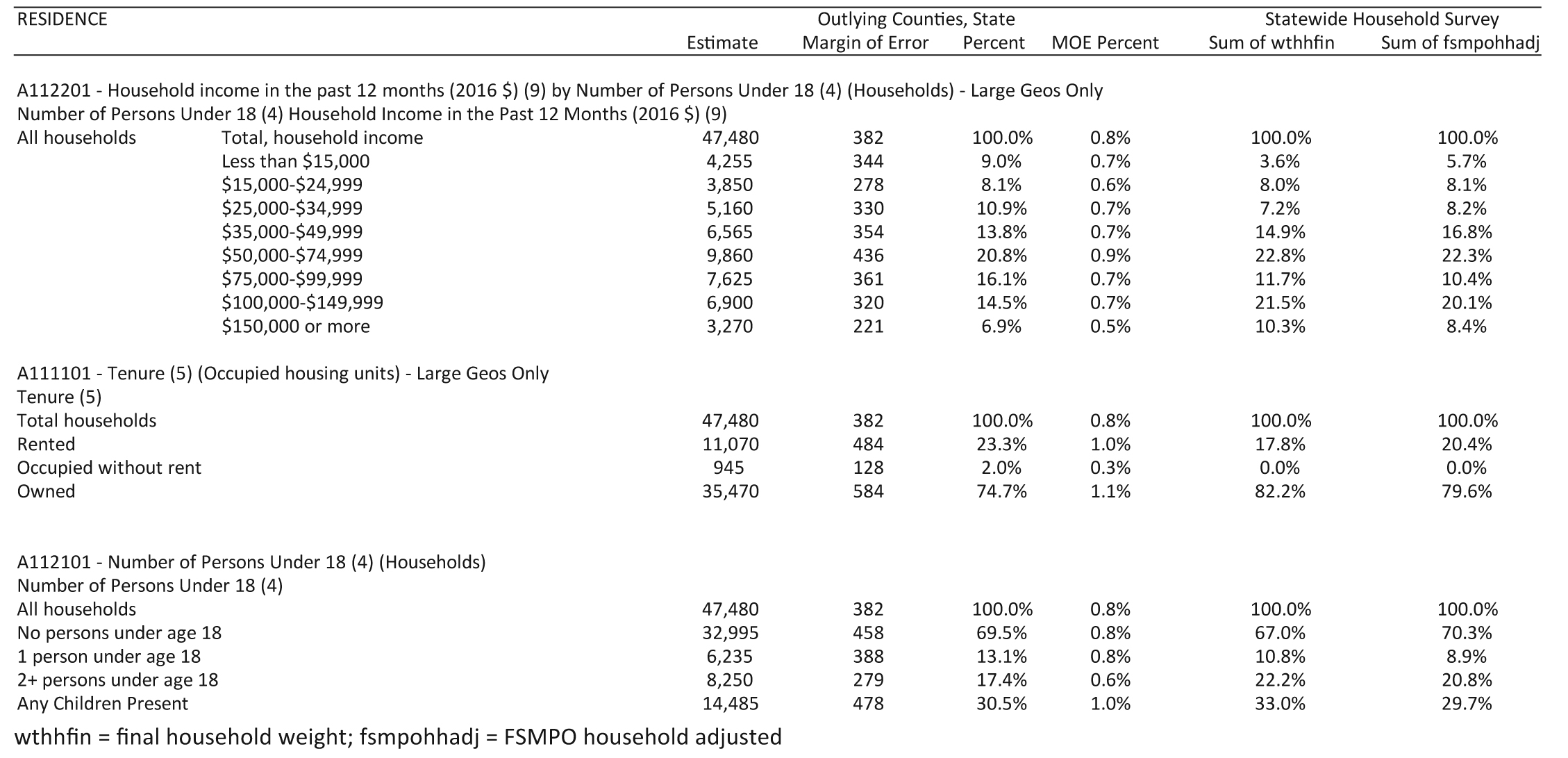
Figure 12.3 and Figure 12.4 show similar comparisons (and similar results) for the two county groups for other household variables. The survey estimates generally follow the same pattern as
Long Description.
The table has 6 columns and 18 rows.The first column is residence. Under the heading Winter County, State, are four columns: estimate, margin of error, percent, and margin of error percent. The sixth column, sum of wthh fin (final household weight), is under the heading Statewide Household Survey. Row details are as follows. Rows 1through 9 are under the heading A112201 Household income in the past 12 months 2016 dollars 9 by Number of Persons Under 18 (4) Households Large geos only; Number of Persons Under 18 (4) Household Income in the Past 12 Months (2016 $) (9); All households. Row 1.Total household income: Estimate 213,520; Margin of error 852; Percent 100.0; Margin of error percent 0.4; Statewide household survey sum of wthh fin 100.0 percent. Row 2. Less than 15,000 dollars: Estimate 19,520; Margin of error 714; Percent 9.1; Margin of error percent 0.3; Statewide household survey sum of wthh fin 8.9 percent. Row 3. 15,000 to 24,999 dollars: Estimate 16,955; Margin of error 788; Percent 7.9; Margin of error percent 0.4; Statewide household survey sum of wthh fin 7.7 percent. Row 4. 25,000 to 34,999 dollars: Estimate 18,900; Margin of error 919; Percent 8.9; Margin of error percent 0.4; Statewide household survey sum of wthh fin 9.1 percent. Row 5. 35,000 to 49,999 dollars: Estimate 26,940; Margin of error 726; Percent 12.6; Margin of error percent 0.3; Statewide household survey sum of wthh fin 11.8 percent. Row 6. 50,000 to 74,999 dollars: Estimate 39,145; Margin of error 1,055; Percent 18.3; Margin of error percent 0.5; Statewide household survey sum of wthh fin 18.6 percent. Row 7. 75,000 to 99,999 dollars: Estimate 29,700; Margin of error 941; Percent 13.9; Margin of error percent 0.4; Statewide household survey sum of wthh fin 17.4 percent. Row 8. 100,000 to 149,999 dollars: Estimate 35,340; Margin of error 997; Percent 16.6; Margin of error percent 0.5; Statewide household survey sum of wthh fin 16.1 percent. Row 9. 150,000 or more: Estimate 27,020; Margin of error 891; Percent 12.7; Margin of error percent 0.4; Statewide household survey sum of wthh fin 10.4 percent. Rows 10 through 13 are under the heading A111101 Tenure 5 Occupied housing units Large geos only; Tenure 5. Row 10. Total households: Estimate 213,520; Margin of error 852; Percent 100.0; Margin of error percent 0.4; Statewide household survey sum of wthh fin 100.0 percent. Row 11. Rented: Estimate 87,435; Margin of error 1,163; Percent 40.9; Margin of error percent 0.5; Statewide household survey sum of wthh fin 44.5 percent. Row 12. Category same as row 10; Occupied without rent: Estimate 1,580; Margin of error 236; Percent 0.7; Margin of error percent 0.1; Statewide household survey sum of wthh fin 0.9 percent. Row 13. Owned: Estimate 124,505; Margin of error 1,379; Percent 58.3; Margin of error percent 0.6; Statewide household survey sum of wthh fin 54.6 percent. Rows 14 through 18 are under the heading A112101 Number of Persons Under 18 (4) Households; Number of Persons Under 18, 4. Row 14. All households: Estimate 213,520; Margin of error 852; Percent 100.0; Margin of error percent 0.4; Statewide household survey sum of wthh fin 100.0 percent. Row 15. No persons under age 18: Estimate 154,180; Margin of error 1,285; Percent 72.2; Margin of error percent 0.5; Statewide household survey sum of wthh fin 72.6 percent. Row 16. 1 person under age 18: Estimate 25,040; Margin of error 1,202; Percent 11.7; Margin of error percent 0.6; Statewide household survey sum of wthh fin 11.9 percent. Row 17. 2 or more persons under age 18: Estimate 34,300; Margin of error 758; Percent 16.1; Margin of error percent 0.3; Statewide household survey sum of wthh fin 15.5 percent. Row 18. Any children present: Estimate 59,340; Margin of error 1,421; Percent 27.8; Margin of error percent 0.7; Statewide household survey sum of wthh fin 27.4 percent.
Long Description.
The table has 6 columns and 18 rows. The first column is residence. Under the heading Outlying Counties, State, are four columns: estimate, margin of error, percent, and margin of error percent. The sixth column, sum of wthh fin (final household weight), is under the heading Statewide Household Survey.Row details are as follows. Rows 1 through 9 are under the heading A112201 Household income in the past 12 months 2016 dollars 9 by Number of Persons Under 18 (4) Households Large geos only; Number of Persons Under 18 (4) Household Income in the Past 12 Months (2016 $) (9) All households. Row 1.Total household income: Estimate 47,480; Margin of error 382; Percent 100.0; Margin of error percent 0.8; Statewide household survey sum of wthh fin 100.0 percent. Row 2. Less than 15,000 dollars: Estimate 4,255; Margin of error 344; Percent 9.0; Margin of error percent 0.7; Statewide household survey sum of wthh fin 3.6 percent. Row 3. 15,000 to 24,999 dollars: Estimate 3,850; Margin of error 278; Percent 8.1; Margin of error percent 0.6; Statewide household survey sum of wthh fin 8.0 percent. Row 4. 25,000 to 34,999 dollars: Estimate 5,160; Margin of error 330; Percent 10.9; Margin of error percent 0.7; Statewide household survey sum of wthh fin 7.2 percent. Row 5. 35,000 to 49,999 dollars: Estimate 6,565; Margin of error 354; Percent 13.8; Margin of error percent 0.7; Statewide household survey sum of wthh fin 14.9 percent. Row 6. 50,000 to 74,999 dollars: Estimate 9,860; Margin of error 436; Percent 20.8; Margin of error percent 0.9; Statewide household survey sum of wthh fin 22.8 percent. Row 7. 75,000 to 99,999 dollars: Estimate 7,625; Margin of error 361; Percent 16.1; Margin of error percent 0.7; Statewide household survey sum of wthh fin 11.7 percent. Row 8. 100,000 to 149,999 dollars: Estimate 6,900; Margin of error 320; Percent 14.5; Margin of error percent 0.7; Statewide household survey sum of wthh fin 21.5 percent. Row 9. 150,000 dollars or more; Estimate 3,270; Margin of error 221; Percent 6.9; Margin of error percent 0.5; Statewide household survey sum of wthh fin 10.3 percent. Rows 10 through 13 are under the heading A111101 Tenure 5 Occupied housing units Large geos only; Tenure 5. Row 10. Total households: Estimate 47,480; Margin of error 382; Percent 100.0; Margin of error percent 0.8; Statewide household survey sum of wthh fin 100.0 percent. Row 11. Rented: Estimate 11,070; Margin of error 484; Percent 23.3; Margin of error percent 1.0; Statewide household survey sum of wthh fin 17.8 percent. Row 12. Occupied without rent: Estimate 945; Margin of error 128; Percent 2.0; Margin of error percent 0.3; Statewide household survey sum of wthh fin 0.0 percent. Row 13. Owned: Estimate 35,470; Margin of error 584; Percent 74.7; Margin of error percent 1.1; Statewide household survey sum of wthh fin 82.2 percent. Rows 14 through 18 are under the heading A112101 Number of Persons Under 18 (4) Households; Number of Persons Under 18, 4. Row 14. All households: Estimate 47,480; Margin of error 382; Percent 100.0; Margin of error percent 0.8; Statewide household survey sum of wthh fin 100.0 percent. Row 15. No persons under age 18: Estimate 32,995; Margin of error 458; Percent 69.5; Margin of error percent 0.8; Statewide household survey sum of wthh fin 67.0 percent. Row 16. 1 person under age 18; Estimate 6,235; Margin of error 388; Percent 13.1; Margin of error percent 0.8; Statewide household survey sum of wthh fin 10.8 percent. Row 17. 2 or more persons under age 18: Estimate 8,250; Margin of error 279; Percent 17.4; Margin of error percent 0.6; Statewide household survey sum of wthh fin 22.2 percent. Row 18. Any children present: Estimate 14,485; Margin of error 478; Percent 30.5; Margin of error percent 1.0; Statewide household survey sum of wthh fin 33.0 percent.
the CTPP data, but there are some meaningful differences. As with the first set of comparisons, the Winter County estimates of the two sources are more closely aligned than the periphery county estimates. (The tables shown in Figures 12.3 and 12.4 can also be accessed via the “Comparison” worksheet of the travel survey weighting spreadsheet.)
David concluded that to get the most out of the household travel survey results, he should develop new weights based on these key variables: household size, number of workers in household, vehicle available, household income, tenure, and persons under age 18.
The challenge that David faced is that when one applies weights to correct for differences along one dimension, the differences along other dimensions can become worse. For instance, when David corrected for differences in the distribution of workers by multiplying the existing weights by the ratio of the CTPP estimate percentages to survey category percentages, the distribution of vehicle availability was much worse.
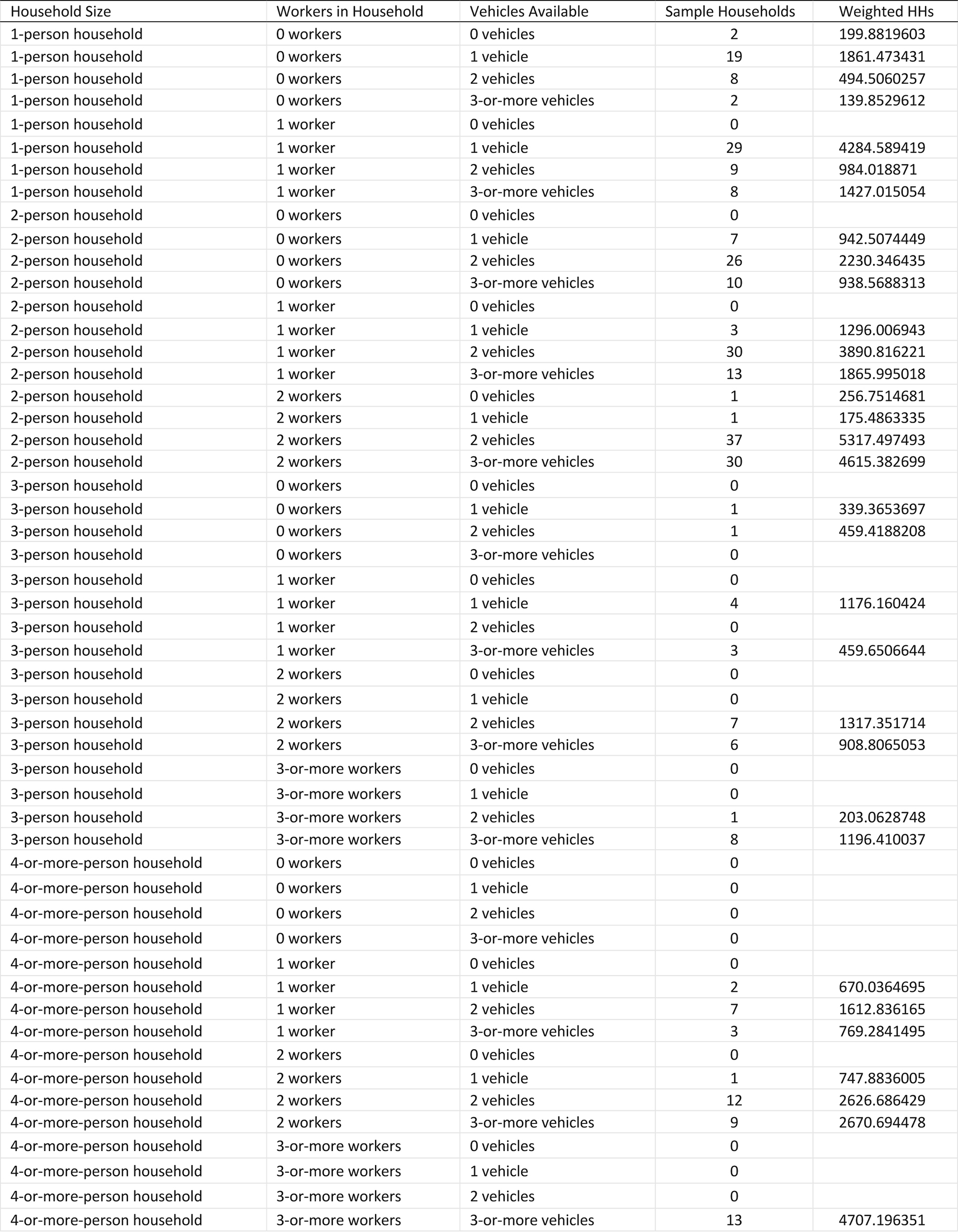
To lessen the impact of this problem, David first turned to the CTPPʼs multidimensional tables. CTPP Table A112305 is a three-way table: household size by number of workers in household by vehicles available. If David could make a similar three-way table of the household survey data, he could simply divide the estimates of each combination of the variables to develop weights that would simultaneously address all three of these variable dimensions.
Unfortunately, the survey data could not support this direct weighting approach because the number of survey records in some of the categories was zero or close to zero, which leads to unstable weights. Figure 12.5 shows the distribution of survey responses for periphery counties for three variables (household size, workers in household, and vehicles available). Many of the variable combinations have no sample households, and many others have only a few.
David concluded he would need to do one or more of the following:
- Combine the categories that are likely to have similar travel behaviors (such as combining all zero-vehicle households, regardless of number of workers or household size).
- Redefine variables to capture travel behavior differences with less-detailed variable combinations.
- Employ iterative proportional fitting to control multiple dimensions.
The first strategy is similar to the geographic combination David employed when he combined the periphery counties. David combined household size and workers categories to reduce the number of cells with very few observations in the table. As an example, for the purpose of weighting, David was willing to combine 3-person households with 4-plus-person households in the periphery counties to a 3-or-more-person definition. Note that this decision does not mean the household size differences between 3- and 4-person households cannot be included in later modeling analyses. The compromise for weighting is used to allow for better descriptive statistics of the population as a whole. The full list of combinations is shown below:
- PA—Periphery Counties, Household Size: 1, Number of Workers in Household: 0
- PB—Periphery Counties, Household Size: 1, Number of Workers in Household: 1
- PC—Periphery Counties, Household Size: 2-4, Number of Workers in Household: 0
- PD—Periphery Counties, Household Size: 2, Number of Workers in Household: 1
- PE—Periphery Counties, Household Size: 2, Number of Workers in Household: 2
- PF—Periphery Counties, Household Size: 3–4+, Number of Workers in Household: 1
- PG—Periphery Counties, Household Size: 3–4+, Number of Workers in Household: 2
- PH—Periphery Counties, Household Size: 3–4+, Number of Workers in Household: 3+
- WA—Winter County, Household Size: 1, Number of Workers in Household: 0
- WB—Winter County, Household Size: 1, Number of Workers in Household: 1
- WC—Winter County, Household Size: 2–4, Number of Workers in Household: 0
Long Description.
The table has 5 columns and 52 rows. The columns include Household Size, Workers in Household, Vehicles Available, Sample Households, and Weighted H Hs. Row details are as follows: Row 1: 1-person household, 0 workers, 0 vehicles, 2, 199.8819603. Row 2: 1-person household, 0 workers, 1 vehicle, 19, 1861.473431. Row 3: 1-person household, 0 workers, 2 vehicles, 8, 494.5060257. Row 4: 1-person household, 0 workers, 3-or-more vehicles, 2, 139.8529612. Row 5: 1-person household, 1 worker, 0 vehicles, 0, blank. Row 6: 1-person household, 1 worker, 1 vehicle, 29, 4284.589419. Row 7: 1-person household, 1 worker, 2 vehicles, 9, 984.018871. Row 8: 1-person household,1 worker, 3-or-more vehicles, 8, 1427.015054. Row 9: 2-person household, 0 workers, 0 vehicles, 0, blank. Row 10: 2-person household, 0 workers, 1 vehicle, 7, 942.5074449. Row 11: 2-person household, 0 workers, 2 vehicle,s 26, 2230.346435. Row 12: 2-person household, 0 workers, 3-or-more vehicles, 10, 938.5688313. Row 13: 2-person household, 1 worker, 0 vehicles, 0, blank. Row 14: 2-person household, 1 worker, 1 vehicle, 3, 1296.006943. Row 15: 2-person household, 1 worker, 2 vehicles, 30, 3890.816221. Row 16: 2-person household, 1 worker, 3-or-more vehicles, 13, 1865.995018. Row 17: 2-person household, 2 workers, 0 vehicles, 1, 256.7514681. Row 18: 2-person household, 2 workers, 1 vehicle, 1, 175.4863335. Row 19: 2-person household, 2 workers, 2 vehicles, 37, 5317.497493. Row 20: 2-person household, 2 workers, 3-or-more vehicles, 30, 4615.382699. Row 21: 3-person household, 0 workers, 0 vehicles, 0, blank. Row 22: 3-person household, 0 workers, 1 vehicle, 1, 339.3653697. Row 23: 3-person household, 0 workers, 2 vehicles, 1, 459.4188208. Row 24: 3-person household, 0 workers, 3-or-more vehicles, 0, blank. Row 25: 3-person household, 1 worker, 0 vehicles, 0, blank. Row 26: 3-person household, 1 worker, 1 vehicle, 4, 1176.160424. Row 27: 3-person household, 1 worker, 2 vehicles, 0, blank. Row 28: 3-person household, 1 worker, 3-or-more vehicles, 3, 459.6506644. Row 29: 3-person household, 2 workers, 0 vehicles, 0, blank. Row 30: 3-person household, 2 workers, 1 vehicle, 0, blank. Row 31: 3-person household, 2 workers, 2 vehicles, 7, 1317.351714. Row 32: 3-person household, 2 workers, 3-or-more vehicles, 6, 908.8065053. Row 33: 3-person household, 3-or-more workers, 0 vehicles, 0, blank. Row 34: 3-person household, 3-or-more workers, 1 vehicle, 0, blank. Row 35: 3-person household, 3-or-more workers, 2 vehicles, 1, 203.0628748. Row 36: 3-person household, 3-or-more workers, 3-or-more vehicles, 8, 1196.410037. Row 37: 4-or-more-person household, 0 workers, 0 vehicles, 0, blank. Row 38: 4-or-more-person household, 0 workers, 1 vehicle, 0, blank. Row 39: 4-or-more-person household, 0 workers, 2 vehicles, 0, blank. Row 40: 4-or-more-person household, 0 workers, 3-or-more vehicles, 0, blank. Row 41: 4-or-more-person household, 1 worker, 0 vehicles, 0, blank. Row 42: 4-or-more-person household, 1 worker, 1 vehicle, 2, 670.0364695. Row 43: 4-or-more-person household, 1 worker, 2 vehicles, 7, 1612.836165. Row 44: 4-or-more-person household, 1 worker, 3-or-more vehicles, 3, 769.2841495. Row 45: 4-or-more-person household, 2 workers, 0 vehicles, 0, blank. Row 46: 4-or-more-person household, 2 workers, 1 vehicle, 1, 747.8836005. Row 47: 4-or-more-person household, 2 workers, 2 vehicles, 12, 2626.686429. Row 48: 4-or-more-person household, 2 workers, 3-or-more vehicles, 9,2670.694478. Row 49: 4-or-more-person household, 3-or-more workers, 0 vehicles, 0, blank. Row 50: 4-or-more-person household, 3-or-more workers, 1 vehicle, 0, blank. Row 51: 4-or-more-person household, 3-or-more workers, 2 vehicles, 0, blank. Row 52: 4-or-more-person household, 3-or-more workers, 3-or-more vehicles, 13, 4707.196351.
- WD—Winter County, Household Size: 2, Number of Workers in Household: 1
- WE—Winter County, Household Size: 2, Number of Workers in Household: 2
- WF—Winter County, Household Size: 3, Number of Workers in Household: 1
- WG—Winter County, Household Size: 3, Number of Workers in Household: 2
- WH—Winter County, Household Size: 3, Number of Workers: 3
- WI—Winter County, Household Size: 4+, Number of Workers: 1
- WJ—Winter County, Household Size: 4+, Number of Workers: 2
- WK—Winter County, Household Size: 4+, Number of Workers: 3+
The second approach David employed was to redefine the variables being used. Rather than relying on individual vehicle availability categories for each combination of household size, number of workers in household, and county grouping, David created a regionwide measure of vehicle availability and sufficiency based on the number of adults in a household and the number of vehicles available to the household. The measure had six categories:
- Vd0—Zero-vehicle households
- Vd1—One vehicle, 2 or more adults
- Ve1—One vehicle, 1 adult
- Vd2—Two or more vehicles, More adults than vehicles
- Ve2—Two or more vehicles, Same number of adults as vehicles
- Vs2—Two or more vehicles, More vehicles than adults
The modified household size/number of workers categorization and the vehicle availability and sufficiency categorization are included in the “HHSurvey_FSMPO” worksheet of the travel survey weighting spreadsheet in the columns that are shaded green.
Iterative proportional fitting (IPF) is a mathematical method for iteratively factoring cross-classified data to match multiple marginal total targets while maintaining as much of the cross-classification as possible. The method is usually credited to Deming and Stefan (1940), but there are probably earlier examples of its usage, and it is referred to by many other names:
- Transportation planners and modelers often refer to this method as the Fratar method, after Thomas Fratar, who introduced it to the field in an early Cleveland Transportation Study.
- Survey researchers often call the method “raking.”
- Economists often refer to it as the “RAS algorithm.”
- Computer scientists have called it “matrix scaling.”
- Others call it “biproportional fitting.”
The method consists of the following steps:
- The input is a multidimensional table that includes the relationships between the different cells in the table and separate target marginal totals.
- The algorithm factors the table along the first dimension so that the summed table elements satisfy the first target marginal total.
- Then, the resulting table is factored along the next dimension so that the summed table elements satisfy the next target marginal total.
- The algorithm repeats the process over and over until the table rows and columns converge on all the marginal targets within an acceptable allowance.
There are R, SAS, and Python modules for applying IPF, and many practitioners have developed Excel VBA routines. In this scenarioʼs workbook in the travel survey weighting spreadsheet, the method is applied using basic Excel without any macros or scripting.
David summarized the CTPP table data to obtain the target marginal total for the modified household size/number of workers in household categories and the target marginal total for the
modified vehicle availability and sufficiency categories. Then he tabulated the weighted survey data to obtain the two-dimensional seed table. The table and row and column target totals were copied into the top of the “Factoring” worksheet (in the travel survey weighting spreadsheet) and then the raking process was completed. The resulting factored table is used as a lookup table to add adjusted weights to the “HHSurvey_FSMPO” worksheet (see columns that are shaded blue). The results of the application of the adjusted weights to the survey data are summarized in Figures 12.6 through 12.9.
Because the full combination of household size, number of workers in household, and vehicle availability and sufficiency did not provide a sufficient sample, David could not directly apply fully corrective weight adjustments. Nevertheless, the weighted survey results were improved by the measures that David took. David could continue the weighting process by bringing more variables into the IPF before finalizing the FSMPO weights.
Long Description.
The table has 7 columns and 16 rows. The first column is residence. Under the heading Winter County, State, there are four columns: estimate, margin of error, percent, and margin of error percent. Under the heading Statewide Household Survey, there are two columns: sum of wthh fin (final household weight) and sum of fsmpohh adj (FSMPO household adjusted). Row details are as follows. Row 1. A112100 Total households 1 Households; Estimate: Estimate 213,520; Margin of error 852; Percent 100.0; Margin of error percent 0.4; Statewide household survey sum of wthh fin 239,026; Statewide household survey sum of fsmpohh adj 239,026. Rows 2 through 6 are under the heading A112106 Household size 5 Households; Household size 5. Row 2. Total households: Estimate 213,520; Margin of error 852; Percent 100.0; Margin of error percent 0.4; Statewide household survey sum of wthh fin 100.0 percent; Statewide household survey sum of fsmpohh adj 100.0 percent. Row 3. 1-person household: Estimate 64,865; Margin of error 1,385; Percent 30.4; Margin of error percent 0.6; Statewide household survey sum of wthh fin 29.5 percent; Statewide household survey sum of fsmpohh adj 30.4 percent. Row 4. 2- person household: Estimate 77,705; Margin of error 1,294; Percent 36.4; Margin of error percent 0.6; Statewide household survey sum of wthh fin 37.7 percent; Statewide household survey sum of fsmpohh adj 36.2 percent. Row 5. 3-person household: Estimate 30,375; Margin of error 1,180; Percent 14.2; Margin of error percent 0.6; Statewide household survey sum of wthh fin 14.3 percent; Statewide household survey sum of fsmpohh adj 14.7 percent. Row 6. Category same as row 2; 4 or more person household: Estimate 40,570; Margin of error 942; Percent 19.0; Margin of error percent 0.4; Statewide household survey sum of wthh fin 18.4; Statewide household survey sum of fsmpohh adj 18.7. Rows 7 through 11 are under the heading A112109 Number of workers in household 6 Households; Number of workers in household 6. Row 7. Total number of workers in household: Estimate 213,520; Margin of error 852; Percent 100.0; Margin of error percent 0.4; Statewide household survey sum of wthh fin 100.0 percent; Statewide household survey sum of fsmpohh adj 100.0 percent. Row 8. 0 workers; Estimate 42,720; Margin of error 987; Percent 20.0; Margin of error percent 0.5; Statewide household survey sum of wthh fin 17.0 percent; Statewide household survey sum of fsmpohh adj 20.0 percent. Row 9. 1 worker: Estimate 81,665; Margin of error 1,536; Percent 38.2; Margin of error percent 0.7; Statewide household survey sum of wthh fin 40.4 percent; Statewide household survey sum of fsmpohh adj 38.2 percent. Row 10. 2 workers: Estimate 74,505; Margin of error 1,464; Percent 34.9; Margin of error percent 0.7; Statewide household survey sum of wthh fin 37.5 percent; Statewide household survey sum of fsmpohh adj 34.9 percent. Row 11. 3 or more workers: Estimate 14,630; Margin of error 711; Percent 6.9; Margin of error percent 0.3; Statewide household survey sum of wthhfin 5.1 percent; Statewide household survey sum of fsmpohh adj 6.9 percent. Rows 12 through 16 are under the heading A111102 Vehicles available 6 Occupied housing units; Vehicles available 6. Row 12. Total vehicles available: Estimate 213,520; Margin of error 852; Percent 100.0; Margin of error percent 0.4; Statewide household survey sum of wthh fin 100.0 percent; Statewide household survey sum of fsmpohh adj 100.0 percent. Row 13. 0 vehicles: Estimate 16,860; Margin of error 769; Percent 7.8; Margin of error percent 0.4; Statewide household survey sum of wthh fin 8.2 percent; Statewide household survey sum of fsmpohh adj 8.5 percent. Row 14. 1 vehicle: Estimate 75,960; Margin of error 1,595; Percent 35.6; Margin of error percent 0.7; Statewide household survey sum of wthh fin 37.8 percent; Statewide household survey sum of fsmpohh adj 35.6 percent. Row 15. 2 vehicles: Estimate 87,080; Margin of error 1,254; Percent 40.8; Margin of error percent 0.6; Statewide household survey sum of wthh fin 36.3 percent; Statewide household survey sum of fsmpohh adj 40.4 percent. Row 16. 3 or more vehicles: Estimate 33,795; Margin of error 987; Percent 15.8; Margin of error percent 0.5; Statewide household survey sum of wthh fin 17.8 percent; Statewide household survey sum of fsmpohh adj 15.6 percent.

Long Description.
The table has 7 columns and 16 rows. The first coumn is residence. Under the heading Outlying Counties, State, there are four columns: estimate, margin of error, percent, and margin of error percent. Under the heading Statewide Household Survey, there are two columns: sum of wthh fin (final household weight) and sum of fsmpohh adj (FSMPO household adjusted). Row details are as follows. Row 1. Category A112100 Total households 1 Households; Estimate: Estimate 47,480; Margin of error 382; Percent 100.0; Margin of error percent 0.8; Statewide household survey sum of wthh fin 50,786; Statewide household survey sum of fsmpohh adj 50,786. Rows 2 through 6 are under the heading A112106 Household size 5 Households; Household size 5. Row 2. Total households: Estimate 47,480; Margin of error 382; Percent 100.0; Margin of error percent 0.8; Statewide household survey sum of wthh fin 100.0 percent; Statewide household survey sum of fsmpohh adj 100.0 percent. Row 3. 1-person household: Estimate 12,465; Margin of error 440; Percent 26.3; Margin of error percent 0.9; Statewide household survey sum of wthh fin 18.5 percent; Statewide household survey sum of fsmpohh adj 26.3 percent. Row 4. 2-person household: Estimate 18,695; Margin of error 450; Percent 39.4; Margin of error percent 0.9; Statewide household survey sum of wthh fin 42.4 percent; Statewide household survey sum of fsmpohh adjj 38.7 percent. Row 5. 3-person household: Estimate 6,930; Margin of error 349; Percent 14.6; Margin of error percent 0.7; Statewide household survey sum of wthh fin 11.9 percent; Statewide household survey sum of fsmpohh adj 11.6 percent. Row 6. 4-or more person household; Estimate 9,390; Margin of error 330; Percent 19.8; Margin of error percent 0.7; Statewide household survey sum of wthh fin 27.2 percent; Statewide household survey sum of fsmpohh adj 23.4 percent. Rows 7 through 11 are under the heading A112109 Number of workers in household 6 Households; Number of workers in household 6. Row 7. Total number of workers in household: Estimate 47,480; Margin of error 382; Percent 100.0; Margin of error percent 0.8; Statewide household survey sum of wthh fin 100.0 percent; Statewide household survey sum of fsmpohh adj 100.0 percent. Row 8. 0 workers: Estimate 11,230; Margin of error 342; Percent 23.7; Margin of error percent 0.7; Statewide household survey sum of wthh fin 15.0 percent; Statewide household survey sum of fsmpohh adj 23.6 percent. Row 9. 1 worker: Estimate 16,525; Margin of error 535; Percent 34.8; Margin of error percent 1.1; Statewide household survey sum of wthh fin 36.3 percent; Statewide household survey sum of fsmpohh adj 34.8 percent. Row 10. 2 workers: Estimate 16,535; Margin of error 452; Percent 34.8; Margin of error percent 0.9; Statewide household survey sum of wthh fin 36.7 percent; Statewide household survey sum of fsmpohh adj 34.8 percent. Row 11. 3-or-more workers: Estimate 3,195; Margin of error 229; Percent 6.7; Margin of error percent 0.5; Statewide household survey sum of wthh fin 12.0 percent; Statewide household survey sum of fsmpohh adj percent 6.7. Rows 12 through 16 are under the heading A111102 Vehicles available 6; Occupied housing units; Vehicles available 6. Row 12. Total vehicles available: Estimate 47,480; Margin of error 382; Percent 100.0; Margin of error percent 0.8; Statewide household survey sum of wthh fin 100.0 percent; Statewide household survey sum of fsmpohh adj 100.0 percent. Row 13. 0 vehicles: Estimate 2,070; Margin of error 215; Percent 4.4; Margin of error percent 0.5; Statewide household survey sum of wthh fin 0.9 percent; Statewide household survey sum of fsmpohh adj 1.4 percent. Row 14. 1 vehicle: Estimate 13,330; Margin of error 485; Percent 28.1; Margin of error percent 1.0; Statewide household survey sum of wthh fin 22.6 percent; Statewide household survey sum of fsmpohh adj 28.1 percent. Row 15. 2 vehicles: Estimate 19,140; Margin of error 534; Percent 40.3; Margin of error percent 1.1; Statewide household survey sum of wthh fin 37.7 percent; Statewide household survey sum of fsmpohh adj 42.2 percent. Row 16. 3-or-more vehicles: Estimate 12,955; Margin of error 471; Percent 27.3; Margin of error percent 1.0; Statewide household survey sum of wthh fin 38.8 percent; Statewide household survey sum of fsmpohh adj 28.3 percent.

Long Description.
The table has 7 columns and 18 rows. The first column is residence. Under the heading Winter County, State, there are four columns: estimate, margin of error, percent, and margin of error percent. Under the heading Statewide Household Survey, there are two columns: sum of wthh fin (final household weight) and sum of fsmpohh adj (FSMPO household adjusted). Row details are as follows. Rows 1 through 9 are under the heading A112201 Household income in the past 12 months 2016 dollars 9 by Number of Persons Under 18 4 Households, Large geos only; Number of PersonsUnder 18 (4) Household Income in the Past 12 Months (2016 $) (9); All households.Row 1. Total household income: Estimate 213,520; Margin of error 852; Percent 100.0; Margin of error percent 0.4; Statewide household survey sum of wthh fin 100.0 percent; Statewide household survey sum of fsmpohh adj 100.0 percent. Row 2. Less than 15,000 dollars: Estimate 19,520; Margin of error 714; Percent 9.1; Margin of error percent 0.3; Statewide household survey sum of wthh fin 8.9 percent; Statewide household survey sum of fsmpohh adj 9.3 percent. Row 3. 15,000 to 24,999 dollars: Estimate 16,955; Margin of error 788; Percent 7.9; Margin of error percent 0.4; Statewide household survey sum of wthh fin 7.7 percent; Statewide household survey sum of fsmpohh adj 7.5 percent. Row 4. 25,000 to 34,999 dollars: Estimate 18,900; Margin of error 919; Percent 8.9; Margin of error percent 0.4; Statewide household survey sum of wthh fin 9.1 percent; Statewide household survey sum of fsmpohh adj 9.3 percent. Row 5. 35,000 to 49,999 dollars: Estimate 26,940; Margin of error 726; Percent 12.6; Margin of error percent 0.3; Statewide household survey sum of wthh fin 11.8 percent; Statewide household survey sum of fsmpohh adj 12.1 percent. Row 6. 50,000 to 74,999 dollars: Estimate 39,145; Margin of error 1,055; Percent 18.3; Margin of error percent 0.5; Statewide household survey sum of wthh fin 18.6 percent; Statewide household survey sum of fsmpohh adj 18.5 percent. Row 7. 75,000 to 99,999 dollars: Estimate 29,700; Margin of error 941; Percent 13.9; Margin of error percent 0.4; Statewide household survey sum of wthh fin 17.4 percent; Statewide household survey sum of fsmpohh adj 17.1 percent. Row 8. 100,000 to 149,999 dollars: Estimate 35,340; Margin of error 997; Percent 16.6; Margin of error percent 0.5; Statewide household survey sum of wthh fin 16.1 percent; Statewide household survey sum of fsmpohh adj 16.2 percent. Row 9. 150,000 dollars or more; Estimate 27,020; Margin of error 891; Percent 12.7; Margin of error percent 0.4; Statewide household survey sum of wthh fin 10.4 percent; Statewide household survey sum of fsmpohh adj 10.0 percent. Rows 10 through 13 are under the heading A111101 Tenure 5 Occupied housing units, Large geos only; Tenure 5. Row 10. Total households: Estimate 213,520; Margin of error 852; Percent 100.0; Margin of error percent 0.4; Statewide household survey sum of wthh fin 100.0 percent; Statewide household survey sum of fsmpohh adj 100.0 percent. Row 11. Rented: Estimate 87,435; Margin of error 1,163; Percent 40.9; Margin of error percent 0.5; Statewide household survey sum of wthh fin 44.5 percent; Statewide household survey sum of fsmpohh adj 43.6 percent. Row 12. Occupied without rent: Estimate 1,580; Margin of error 236; Percent 0.7; Margin of error percent 0.1; Statewide household survey sum of wthh fin 0.9 percent; Statewide household survey sum of fsmpohh adj 0.8 percent. Row 13. Owned: Estimate 124,505; Margin of error 1,379; Percent 58.3; Margin of error percent 0.6; Statewide household survey sum of wthh fin 54.6 percent; Statewide household survey sum of fsmpohh adj 55.6 percent. Rows 14 through 18 are under the heading A112101 Number of Persons Under 18 (4) Households; Number of Persons Under 18, 4. Row 14. All households: Estimate 213,520; Margin of error 852; Percent 100.0; Margin of error percent 0.4; Statewide household survey sum of wthh fin 100.0 percent; Statewide household survey sum of fsmpohh adj 100.0 percent. Row 15. No persons under age 18: Estimate 154,180; Margin of error 1,285; Percent 72.2; Margin of error percent 0.5; Statewide household survey sum of wthh fin 72.6 percent; Statewide household survey sum of fsmpohh adj 73.2 percent. Row 16. 1 person under age 18: Estimate 25,040; Margin of error 1,202; Percent 11.7; Margin of error percent 0.6; Statewide household survey sum of wthh fin 11.9 percent; Statewide household survey sum of fsmpohh adj 11.8 percent. Row 17. 2 or more persons under age 18: Estimate 34,300; Margin of error 758; Percent 16.1; Margin of error percent 0.3; Statewide household survey sum of wthh fin 15.5 percent; Statewide household survey sum of fsmpohh adj 15.0 percent. Row 18. Any children present: Estimate 59,340; Margin of error 1,421; Percent 27.8; Margin of error percent 0.7; Statewide household survey sum of wthh fin 27.4 percent; Statewide household survey sum of fsmpohh adj 26.8 percent.
Long Description.
The table has 7 columns and 18 rows.The first coumn is residence. Under the heading Outlying Counties, State, there are four columns: estimate, margin of error, percent, and margin of error percent. Under the heading Statewide Household Survey, there are two columns: sum of wthh fin (final household weight) and sum of fsmpohh adj (FSMPO household adjusted). Row details are as follows. Rows 1 through 9 are under the heading A112201 Household income in the past 12 months 2016 dollars 9 by Number of Persons Under 18 (4) Households Large geos only; Description Number of Persons Under 18 (4) Household Income in the Past 12 Months (2016 $) (9)All households. Row 1. Total household income: Estimate 47,480; Margin of error 382; Percent 100.0; Margin of error percent 0.8; Statewide household survey sum of wthh fin 100.0 percent; Statewide household survey sum of fsmpohh adj 100.0 percent. Row 2. Less than 15,000 dollars: Estimate 4,255; Margin of error 344; Percent 9.0; Margin of error percent 0.7; Statewide household survey sum of wthh fin 3.6 percent; Statewide household survey sum of fsmpohh adj 5.7 percent. Row 3. 15,000 to 24,999 dollars: Estimate 3,850; Margin of error 278; Percent 8.1; Margin of error percent 0.6; Statewide household survey sum of wthh fin 8.0 percent; Statewide household survey sum of fsmpohh adj 8.1 percent. Row 4. 25,000 to 34,999 dollars: Estimate 5,160; Margin of error 330; Percent 10.9; Margin of error percent 0.7; Statewide household survey sum of wthh fin 7.2 percent; Statewide household survey sum of fsmpohh adj 8.2 percent. Row 5. 35,000 to 49,999 dollars: Estimate 6,565; Margin of error 354; Percent 13.8; Margin of error percent 0.7; Statewide household survey sum of wthh fin 14.9 percent; Statewide household survey sum of fsmpohh adj 16.8 percent. Row 6. 50,000 to 74,999 dollars: Estimate 9,860; Margin of error 436; Percent 20.8; Margin of error percent 0.9; Statewide household survey sum of wthh fin 22.8 percent; Statewide household survey sum of fsmpohh adj 22.3 percent. Row 7. 75,000 to 99,999 dollars: Estimate 7,625; Margin of error 361; Percent 16.1; Margin of error percent 0.7; Statewide household survey sum of wthh fin 11.7 percent; Statewide household survey sum of fsmpohh adj 10.4 percent. Row 8. 100,000 to 149,999 dollars: Estimate 6,900; Margin of error 320; Percent 14.5; Margin of error percent 0.7; Statewide household survey sum of wthh fin 21.5 percent; Statewide household survey sum of fsmpohh adj 20.1 percent. Row 9. 150,000 dollars or more: Estimate 3,270; Margin of error 221; Percent 6.9; Margin of error percent 0.5; Statewide household survey sum of wthh fin 10.3 percent; Statewide household survey sum of fsmpohh adj 8.4 percent. Rows 10 through 13 are under the heading A111101 Tenure 5 Occupied housing units, Large geos only; Tenure 5. Row 10. Total households: Estimate 47,480; Margin of error 382; Percent 100.0; Margin of error percent 0.8; Statewide household survey sum of wthh fin 100.0 percent; Statewide household survey sum of fsmpohh adj 100.0 percent. Row 11. Rented: Estimate 11,070; Margin of error 484; Percent 23.3; Margin of error percent 1.0; Statewide household survey sum of wthh fin 17.8 percent; Statewide household survey sum of fsmpohh adj 20.4 percent . Row 12. Occupied without rent: Estimate 945; Margin of error 128; Percent 2.0; Margin of error percent 0.3; Statewide household survey sum of wthh fin 0.0 percent; Statewide household survey sum of fsmpohh adj 0.0 percent. Row 13. Owned: Estimate 35,470; Margin of error 584; Percent 74.7; Margin of error percent 1.1; Statewide household survey sum of wthh fin 82.2 percent; Statewide household survey sum of fsmpohh adj 79.6 percent. Rows 14 through 18 are under the heading A112101 Number of Persons Under 18 (4) Households; Number of Persons Under 18 (4). Row 14. All households: Estimate 47,480; Margin of error 382; Percent 100.0; Margin of error percent 0.8; Statewide household survey sum of wthh fin 100.0 percent; Statewide household survey sum of fsmpohh adj 100.0 percent. Row 15. No persons under age 18: Estimate 32,995; Margin of error 458; Percent 69.5; Margin of error percent 0.8; Statewide household survey sum of wthh fin 67.0 percent; Statewide household survey sum of fsmpohh adj 70.3 percent. Row 16. 1 person under age 18: Estimate 6,235; Margin of error 388; Percent 13.1; Margin of error percent 0.8; Statewide household survey sum of wthh fin 10.8 percent; Statewide household survey sum of fsmpohh adj 8.9 percent. Row 17. 2 or more persons under age 18: Estimate 8,250; Margin of error 279; Percent 17.4; Margin of error percent 0.6; Statewide household survey sum of wthh fin 22.2 percent; Statewide household survey sum of fsmpohh adj 20.8 percent. Row 18. Any children present: Estimate 14,485; Margin of error 478; Percent 30.5; Margin of error percent 1.0; Statewide household survey sum of wthh fin 33.0 percent; Statewide household survey sum of fsmpohh adj 29.7 percent.


