Census Data Field Guide for Transportation Applications (2025)
Chapter: 8 Uses of Census Data

CHAPTER 8
Uses of Census Data
An efficient and well-performing transportation system contributes significantly to the nationʼs economy facilitating the movement of people and goods. In recent years, emerging trends that have rapidly transformed the transportation field include:
- Autonomous vehicles (passenger and freight),
- Pervasive connectivity (vehicle to vehicle, vehicle to infrastructure, and person to infrastructure),
- Micromobility (shared bikes and shared scooters),
- Sensing technologies (such as cameras, speed monitors, and air quality sensors),
- Mobile applications (for facilitating mobility and multimodal travel), and
- Data (large streams of data, analytics, and visualization).
The changes brought about by technology and the smartphone revolution have had important impacts on online shopping. Together with the emergence of TNCs, technology and smartphones have changed the way people live, work, shop, and play with profound implications for transportation investment, policy, and operational decisions. One example of this change is the decrease in the proportion of licensed drivers among the 55-and-under age cohort in 2014 as compared to 1983 (Sivak and Schoettle 2016).
These changes in travel behavior need to be measured accurately to ensure that policy decisions happen in a data-driven context. However, collecting data on travel behavior is also becoming more challenging and is hampered by low survey response rates and high rates of survey attrition. Therefore, it is critical to integrate different sources of travel behavior data to provide estimates in a consistent, reliable, and sustainable manner.
An FHWA report on data availability and gaps related to our understanding of travel behavior highlights the need for data fusion techniques to overcome these gaps (Tawfik and Zohdy 2017). Census data, even in this age of big data, offer tremendous value and insights to help overcome the gaps in data availability identified by FHWA. The various data products released by the Census Bureau and its extensions provide information and insights that will help in making data-driven policy decisions to address changes in travel behavior.
Transportation agencies are facing significant challenges in preparing for and responding to changes in travel behavior because of increasing financial and technical constraints. Additionally, upcoming changes in how the Census Bureau currently releases data and its plans to incorporate differential privacy in data releases underscore the need for transportation analysts to better understand how to use Census Bureau data, understand the implications of data suppression, and assess how skewed results can prevent meaningful analysis. All these changes call for the development of a resource that is practical and relevant and encourages both new entrants to the profession and experienced professionals to use various census data products and apply them to solve transportation problems.
This research effort was motivated by the need to develop resources that will help a wide range of agencies including FHWA, state DOTs, transit operators, and MPOs. These resources can be used to evaluate the strengths and weaknesses of census data products and provide advice on how to best use these data in their own right or in conjunction with other data sources.
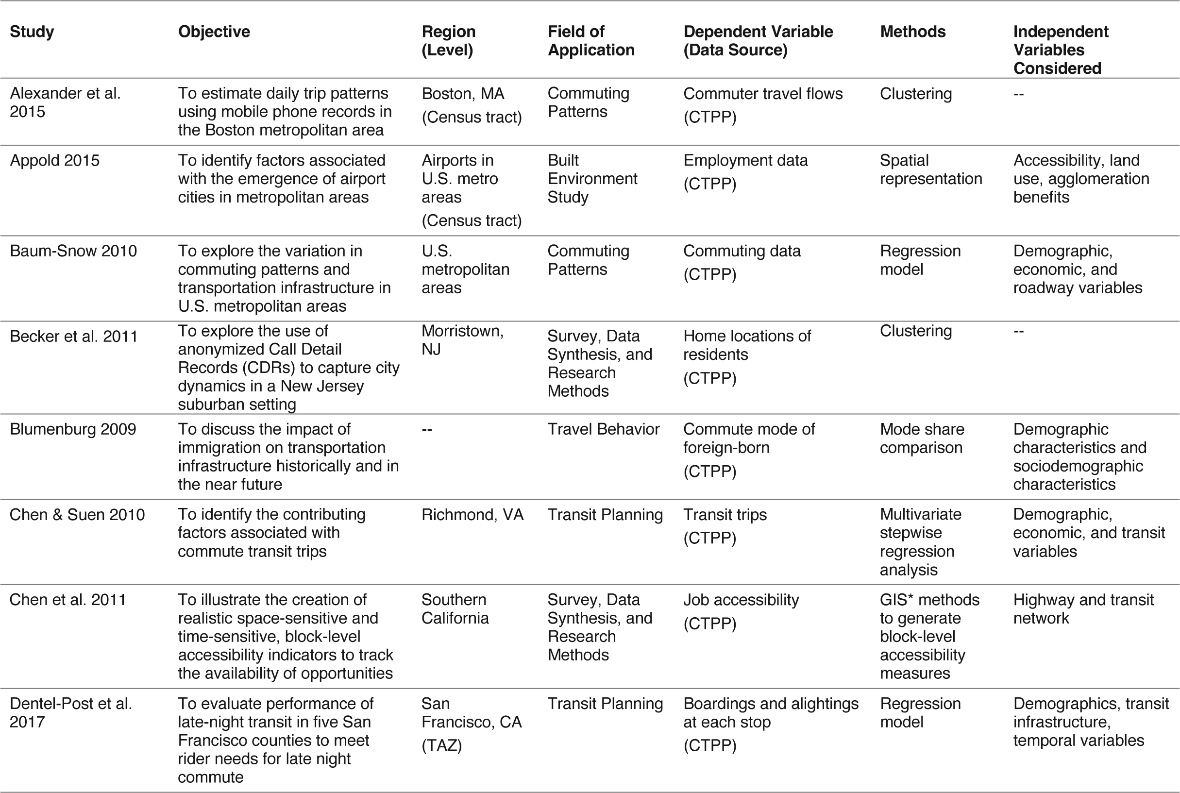
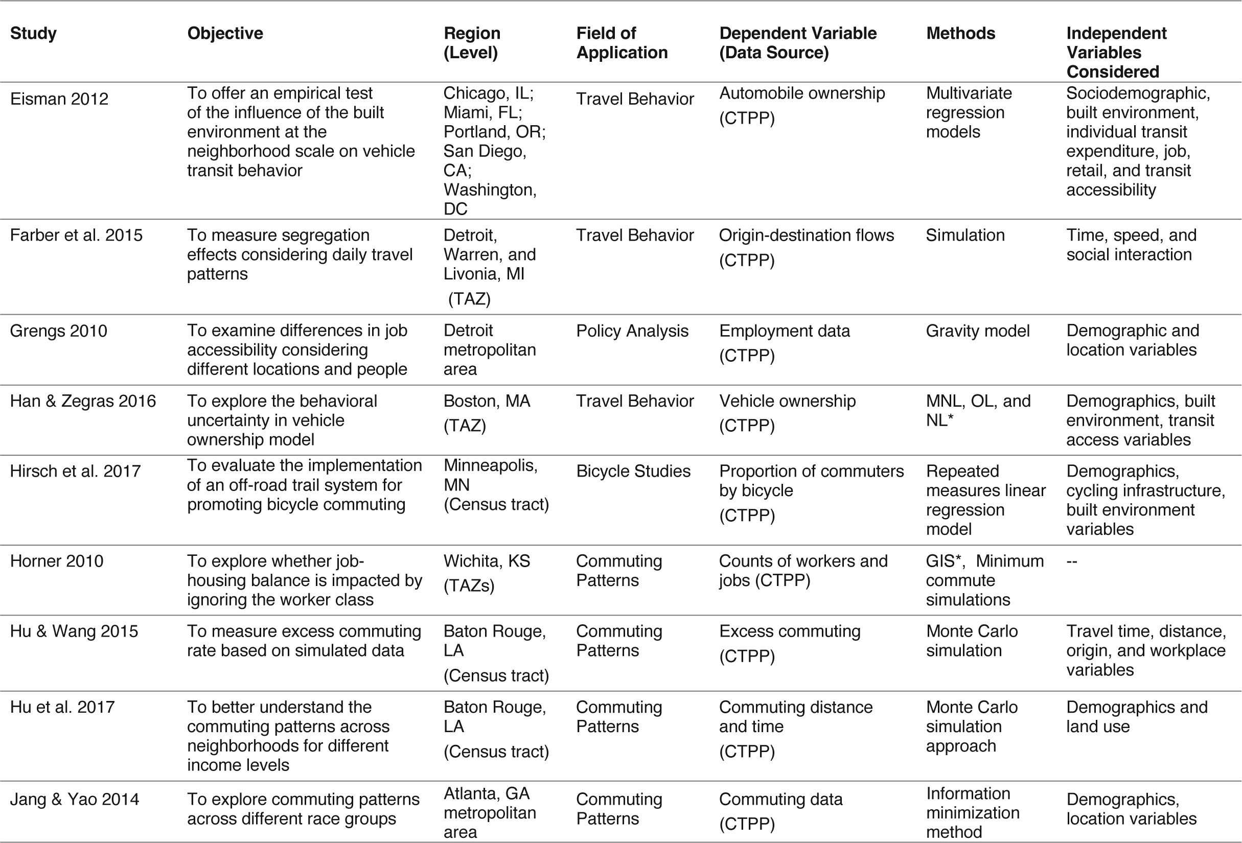
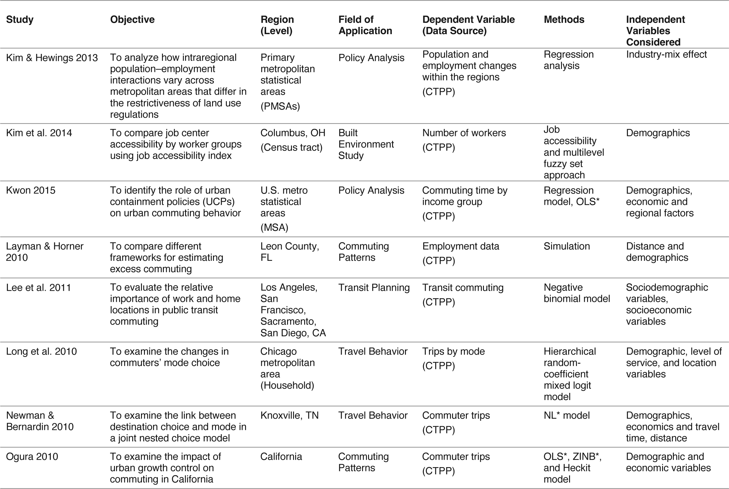
To support the overall objective of the research effort, the research team reviewed how census data products have been applied in various areas of transportation. The literature review examines the application of various census data sources for transportation applications including the AASHTO CTPP, the ACS, the LEHD program, and the PUMS and PUMA. A preliminary review of transportation applications of these census data revealed a large number of studies over the last several decades. To present a review that would be practical and relevant for future transportation agency use, the research team limited its review to papers or reports published since 2010. “The CTPP Workplace Data for Transportation Planning: A Systematic Review” provides an exhaustive review of studies prior to 2010 (Seo et al. 2017).
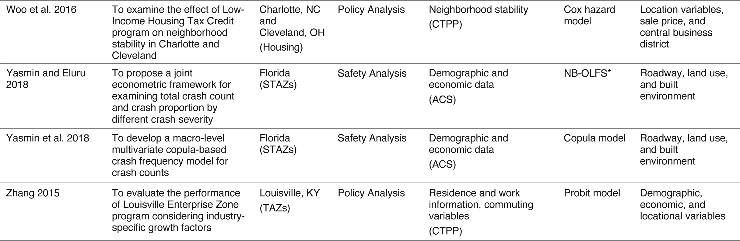
The research team organized its review of census-related studies into two study types. The first type of study employs census-related data sources as the primary data source and the primary variable of interest of the study is compiled using a census-related data source. The second type of study employs census-related data sources as a secondary data source to augment analysis of research-driven data compiled from other sources. In this second type of study, the breadth of research areas covered is wider than in the first type of study. Specifically, researchers rely on CTPP or ACS data to generate buffer- or neighborhood-level information to model various transportation-system-related variables. For example, ACTS variables, such as commuting mode share and/or median household income at a census tract level, are employed to analyze transportation safety variables such as crash frequency (see Yasmin et al. 2018, Yasmin and Eluru 2018).
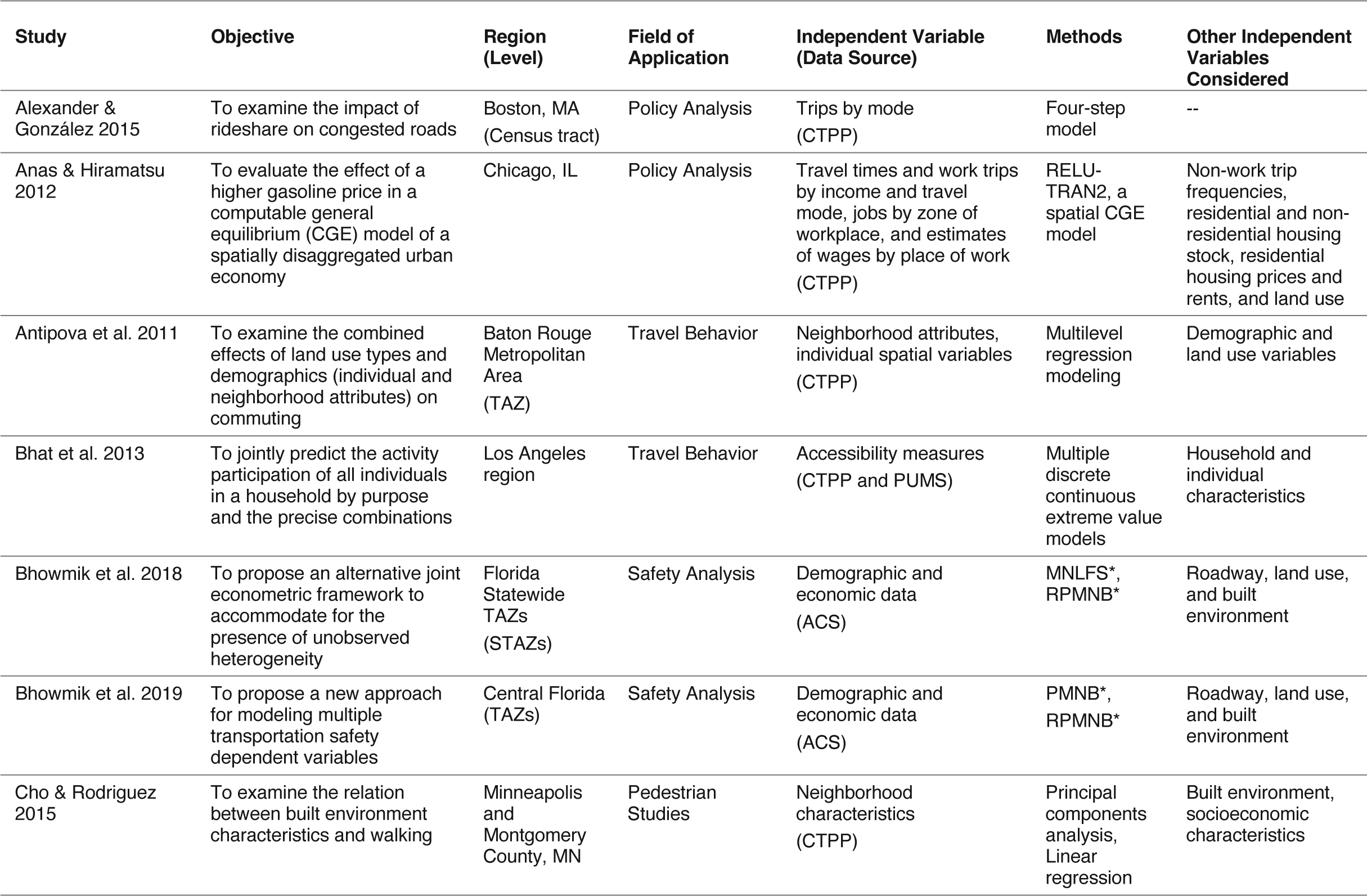
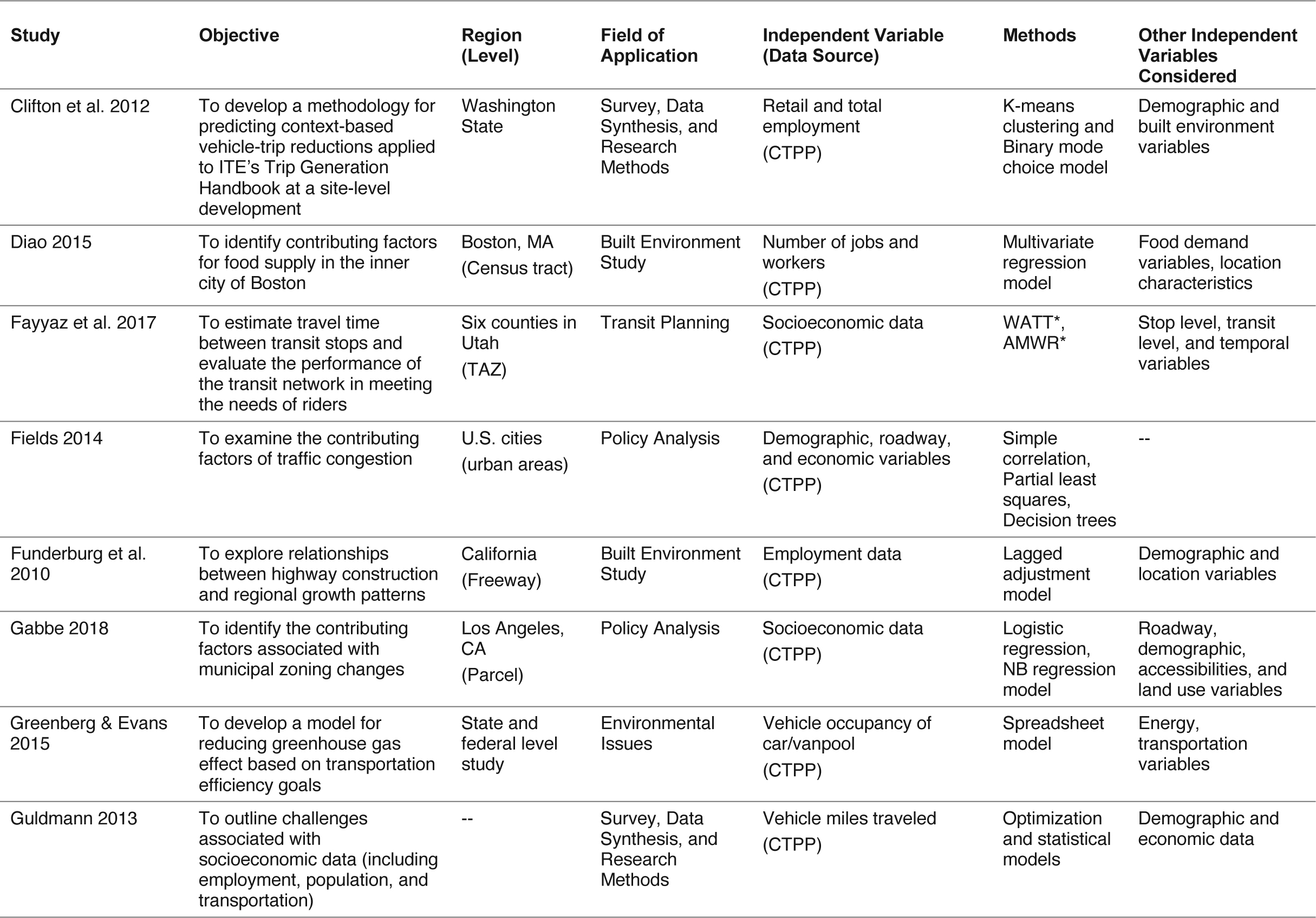
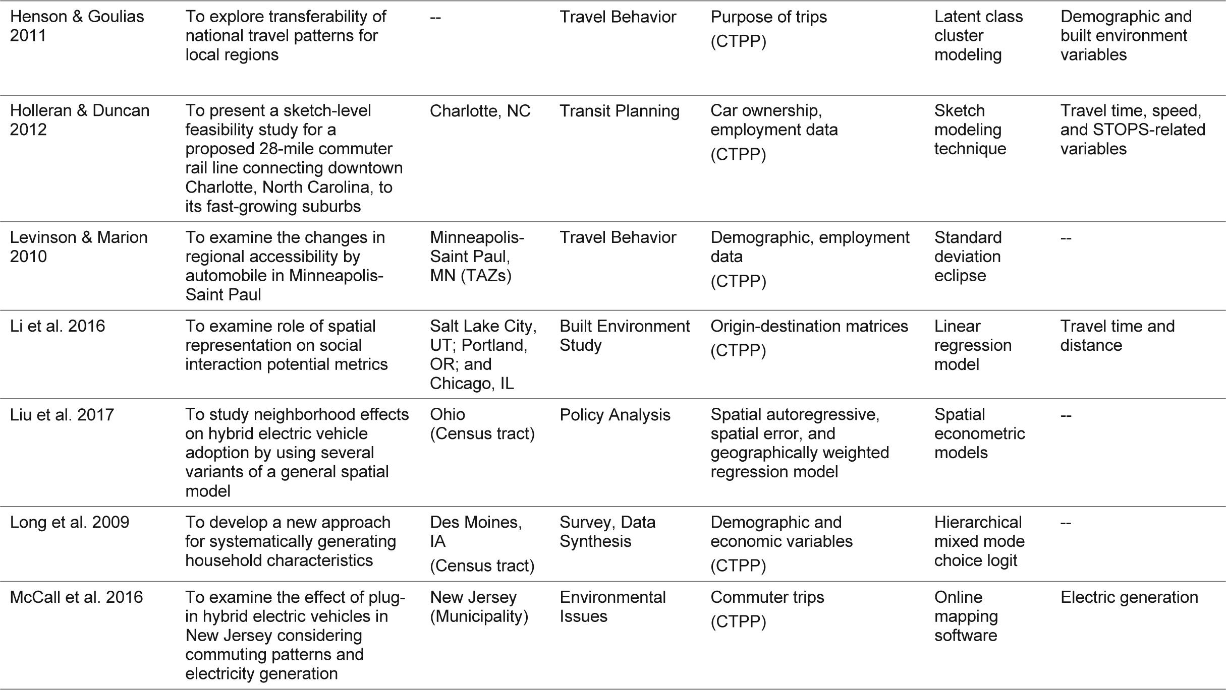
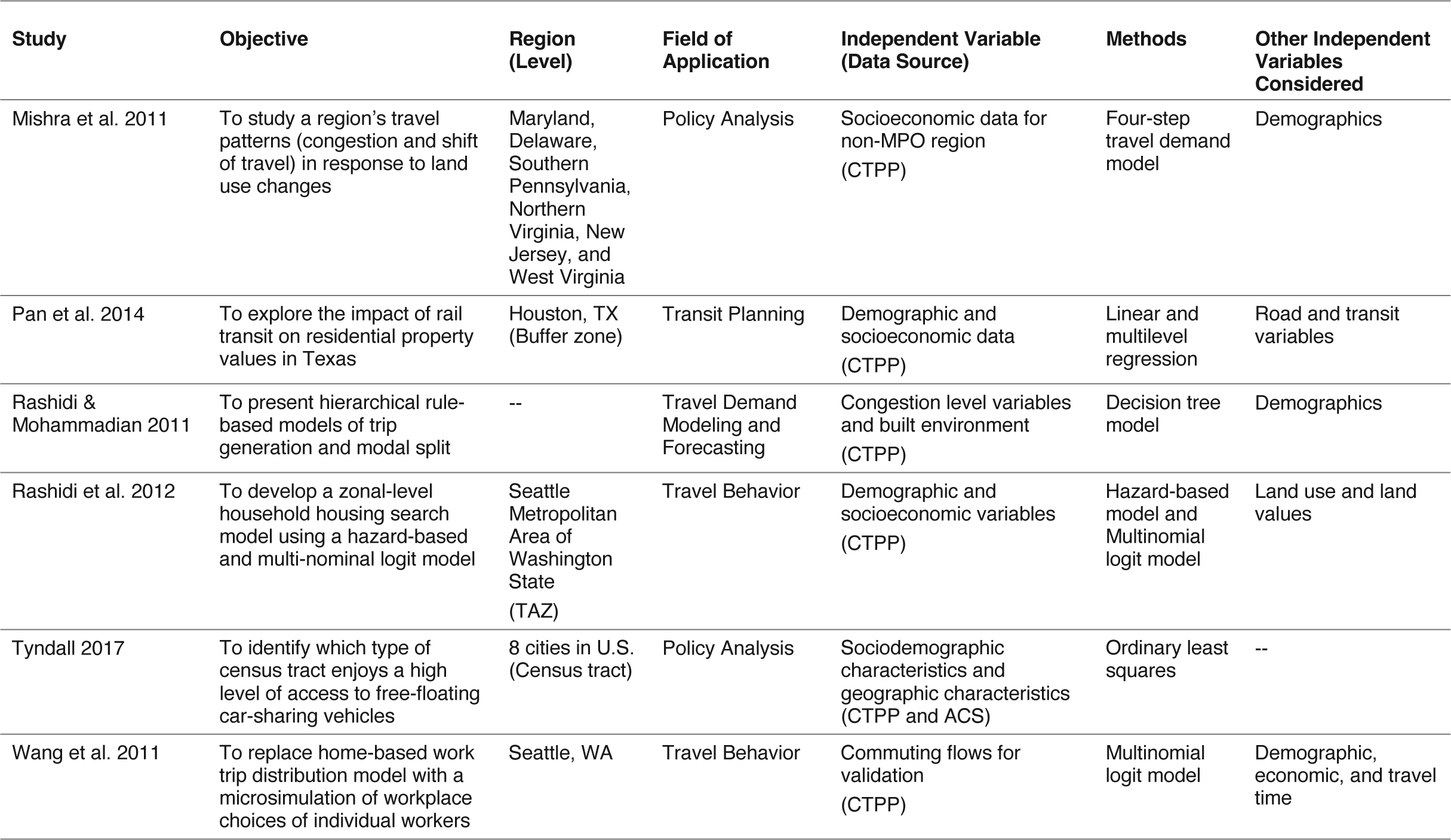
Table 8.1 and Table 8.2 provide a summary of the studies considering census-related data for transportation applications. The tables provide information on the study objectives, the spatial resolution of the analysis, the transportation field of application, the dependent variable of interest (and the data source employed), the research methodology used, and the various independent variables considered. These two tables document examples from the recent literature that provide interesting findings in a wide range of census data uses: by geography, by topic area of interest, by the dependent variable used, and by the research method applied.
8.1 Spatial Resolution
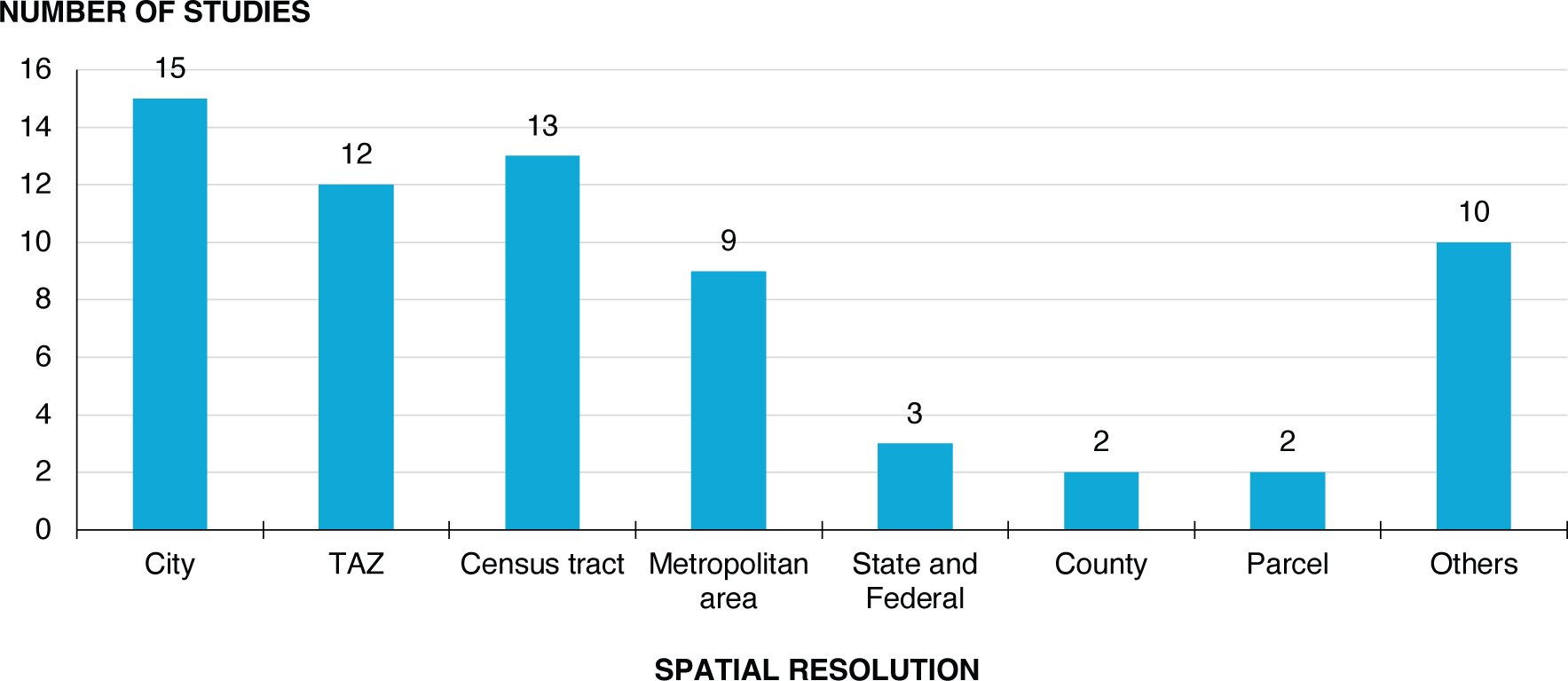
The spatial resolution adopted in research that uses census-related data is influenced by the research objectives. The research efforts that are summarized in Tables 8.1 and 8.2 adopted various levels of spatial resolution for their analyses to be consistent with the broad range of spatial resolution at which census data are available. Census data are available at levels of spatial resolution including state, county, city, MSA, tract, PUMA code based on the 2010 census, TAD, and TAZ.
A summary of the distribution of spatial resolution usage in the studies (a few state and national level studies are categorized “State and Federal”) is presented in Figure 8.1. City, census tract, and TAZ were the three most commonly adopted levels of spatial resolution.
8.2 Topic Area
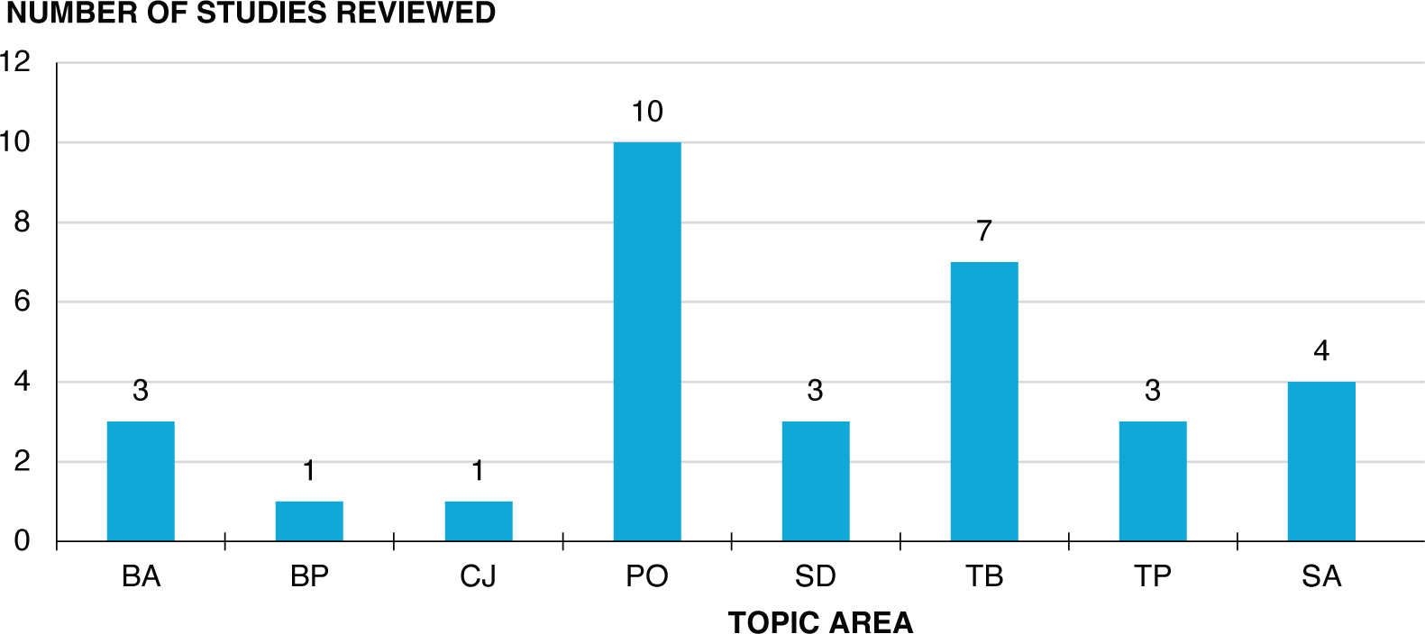
Census-related data sources have been widely employed across various topic areas of transportation. Figure 8.2 and Figure 8.3 provide an overview of the distribution of these topic areas in the literature review across the two types of studies. The first type of study is most often conducted in the fields of commuting patterns and travel behavior. The second type of study is undertaken most commonly in the research fields of policy analysis and travel behavior.
(continued on next page)
(continued on next page)
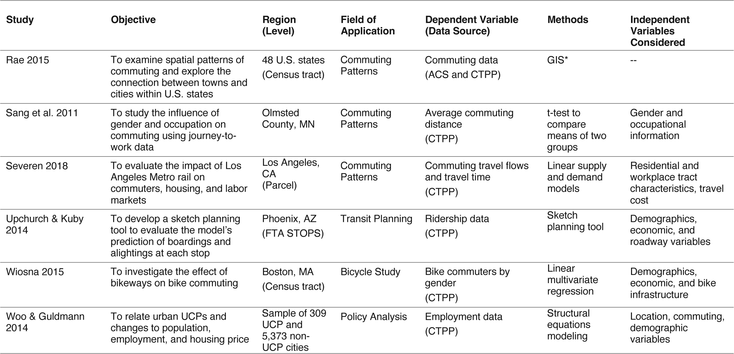
*MNL = multinomial logit, OL = ordered logit, NL = nested logit; OLS = Ordinary least square, GIS = Geographical information system, ZINB = Zero inflated negative binomial model
Long Description.
The table has 7 columns and 31 rows. The columns include the study citation, objective, region (level), field of application, dependent variable (data source), methods, and independent variables considered. Row details are as follows. Row 1. Alexander et al. (2015); To estimate daily trip patterns using mobile phone records in the Boston metropolitan area; Boston, MA (Census tract); Commuting Patterns; Commuter travel flows (CTPP); Clustering, no data. Row 2. Appold 2015; To identify factors associated with the emergence of airport cities in metropolitan areas; Airports in U.S. metro areas (Census tract); Built Environment Study; Employment data (CTPP); Spatial representation; Accessibility, land use, agglomeration benefits. Row 3. Baum-Snow 2010; To explore the variation in commuting patterns and transportation infrastructure in U.S. metropolitan areas; U.S. metropolitan areas; Commuting Patterns; Commuting data (CTPP); Regression model; Demographic, economic, and roadway variables. Row 4. Becker et al. 2011. To explore the use of anonymized Call Detail Records (CDRs) to capture city dynamics in a New Jersey suburban setting; Morristown, NJ; Survey, Data Synthesis, and Research Methods; Home locations of residents (CTPP); Clustering; no data. Row 5. Blumenburg 2009; To discuss the impact of immigration on transportation infrastructure historically and in the near future; no data; Travel Behavior; Commute mode of foreign-born (CTPP); Mode share comparison; Demographic characteristics and sociodemographic characteristics. Row 6. Chen and Suen 2010; To identify the contributing factors associated with commute transit trips; Richmond, VA; Transit Planning; Transit trips (CTPP); Multivariate stepwise regression analysis; Demographic, economic, and transit variables. Row 7. Chen et al. 2011; To illustrate the creation of realistic space-sensitive and time-sensitive, block-level accessibility indicators to track the availability of opportunities; Southern California; Survey, Data Synthesis, and Research Methods; Job accessibility (CTPP); GIS (note cue: star) methods to generate block-level accessibility measures; Highway and transit network. Row 8. Dentel-Post et al. 2017; To evaluate performance of late-night transit in five San Francisco counties to meet rider needs for late night commute. San Francisco, CA (TAZ); Transit Planning; Boardings and alightings at each stop (CTPP); Regression model; Demographics, transit infrastructure, temporal variables. Row 9. Eisman 2012; To offer an empirical test of the influence of the built environment at the neighborhood scale on vehicle transit behavior; Chicago, IL; Miami, FL; Portland, OR; San Diego, CA; Washington, DC; Travel Behavior; Automobile ownership (CTPP); Multivariate regression models; Sociodemographic, built environment, individual transit expenditure, job, retail, and transit accessibility. Row 10. Farber et al. 2015; To measure segregation effects considering daily travel patterns; Detroit, Warren, and Livonia, MI (TAZ); Travel Behavior; Origin-destination flows (CTPP); Simulation; Time, speed, and social interaction. Row 11. Grengs 2010 ; To examine differences in job accessibility considering different locations and people; Detroit metropolitan area; Policy Analysis; Employment data; (CTPP); Gravity model; Demographic and location variables. Row 12. Han & Zegras 2016; To explore the behavioral uncertainty in vehicle ownership model; Boston, MA (TAZ); Travel Behavior; Vehicle ownership (CTPP); MNL, OL, and NL (note cue: star); Demographics, built environment, transit access variables. Row 13. Hirsch et al. 2017; To evaluate the implementation of an off-road trail system for promoting bicycle commuting; Minneapolis, MN (Census tract); Bicycle Studies; Proportion of commuters by bicycle (CTPP); Repeated measures linear regression model; Demographics, cycling infrastructure, built environment variables. Row 14. Horner 2010; To explore whether job-housing balance is impacted by ignoring the worker class; Wichita, KS (TAZs); Commuting Patterns; Counts of workers and jobs (CTPP); G I S (note cue: star), Minimum commute simulations; no data. Row 15. Hu and Wang 2015; To measure excess commuting rate based on simulated data; Baton Rouge, LA (Census tract); Commuting Patterns; Excess commuting (CTPP); Monte Carlo simulation; Travel time, distance, origin, and workplace variables. Row 16. Hu et al. 2017; To better understand the commuting patterns across neighborhoods for different income levels; Baton Rouge, LA (Census tract); Commuting Patterns; Commuting distance and time (CTPP); Monte Carlo simulation approach; Demographics and land use. Row 17. Jang and Yao 2014; To explore commuting patterns across different race groups; Atlanta, GA metropolitan area; Commuting Patterns; Commuting data (CTPP); Information minimization method; Demographics, location variables. Row 18. Kim and Hewings 2013; To analyze how intraregional population–employment interactions vary across metropolitan areas that differ in the restrictiveness of land use regulations; Primary metropolitan statistical areas (PMSAs); Policy Analysis; Population and employment changes within the regions (CTPP); Regression analysis; Industry-mix effect. Row 19. Kim et al. 2014; To compare job center accessibility by worker groups using job accessibility index; Columbus, OH (Census tract); Built Environment Study; Number of workers (CTPP); Job accessibility and multilevel fuzzy set approach; Demographics. Row 20. Kwon 2015; To identify the role of urban containment policies (UCPs) on urban commuting behavior; U.S. metro statistical areas (MSA); Policy Analysis; Commuting time by income group (CTPP); Regression model, OLS (note cue: star); Demographics, economic and regional factors. Row 21. Layman & Horner 2010; To compare different frameworks for estimating excess commuting; Leon County, FL; Commuting Patterns; Employment data (CTPP); Simulation; Distance and demographics. Row 22. Lee et al. 2011; To evaluate the relative importance of work and home locations in public transit commuting; Los Angeles, San Francisco, Sacramento, San Diego, C A; Transit Planning; Transit commuting (CTPP); Negative binomial model; Sociodemographic variables, socioeconomic variables. Row 23. Long et al. 2010; To examine the changes in commuters’ mode choice; Chicago metropolitan area (Household); Travel Behavior; Trips by mode (CTPP); Hierarchical random-coefficient mixed logit model; Demographic, level of service, and location variables. Row 24. Newman and Bernardin 2010; To examine the link between destination choice and mode in a joint nested choice model; Knoxville, TN; Travel Behavior; Commuter trips (CTPP); NL(note cue: star) model; Demographics, economics and travel time, distance. Row 25. Ogura 2010 ; To examine the impact of urban growth control on commuting in California; California; Commuting Patterns; Commuter trips (CTPP); OLS (star note cue), ZINB (star note cue), and Heckit model; Demographic and economic variables. Row 26. Rae 2015; To examine spatial patterns of commuting and explore the connection between towns and cities within U.S. states; 48 U.S. states (Census tract); Commuting Patterns; Commuting data (ACS and CTPP) GIS (star note cue); no data. Row 27. Sang et al. 2011; To study the influence of gender and occupation on commuting using journey-to-work data; Olmsted County, MN; Commuting Patterns; Average commuting distance (CTPP); t-test to compare means of two groups; Gender and occupational information. Row 28. Severen 2018; To evaluate the impact of Los Angeles Metro rail on commuters, housing, and labor markets; Los Angeles, CA (Parcel); Commuting Patterns; Commuting travel flows and travel time (CTPP); Linear supply and demand models; Residential and workplace tract characteristics, travel cost. Row 29. Upchurch and Kuby 2014; To develop a sketch planning tool to evaluate the model’s prediction of boardings and alightings at each stop; Phoenix, AZ (FTA STOPS); Transit Planning; Ridership data (CTPP); Sketch planning tool; Demographics, economic, and roadway variables. Row 30. Wiosna 2015; To investigate the effect of bikeways on bike commuting; Boston, MA (Census tract); Bicycle Study; Bike commuters by gender (CTPP); Linear multivariate regression; Demographics, economic, and bike infrastructure. Row 31. Woo and Guldmann 2014; To relate urban UCPs and changes to population, employment, and housing price; Sample of 309 UCP and 5,373 non-UCP cities; Policy Analysis; Employment data (CTPP); Structural equations modeling; Location, commuting, demographic variables.
(continued on next page)
(continued on next page)
*PMNB = Panel mixed negative binomial model,RPMNB = Random parameter multivariate negative binomial model,NB-OLFS = Negative binomial-ordered logit fractional split model, MNLFS = Multinomial logit fractional split model, WATT = Weighted average travel time, AMWR = Average-to-median WATT ratio, NB = Negative binomial
Long Description.
The table has 7 columns and 33 rows. The columns include the study citation, objective, region (level), field of application, independent variable (data source), methods, and other independent variables considered. Row details are as follows. Row 1: Alexander and González 2015; To examine the impact of rideshare on congested roads; Boston, MA (Census tract); Policy Analysis; Trips by mode (CTPP); Four-step model; no data. Row 2: Anas and Hiramatsu 2012; To evaluate the effect of a higher gasoline price in a computable general equilibrium (CGE) model of a spatially disaggregated urban economy; Chicago, IL; Policy Analysis; Travel times and work trips by income and travel mode, jobs by zone of workplace, and estimates of wages by place of work (CTPP); RELU-TRAN2, a spatial CGE model; Non-work trip frequencies, residential and non-residential housing stock, residential housing prices and rents, and land use. Row 3: Antipova et al. 2011; To examine the combined effects of land use types and demographics (individual and neighborhood attributes) on commuting; Baton Rouge Metropolitan Area (TAZ); Travel Behavior; Neighborhood attributes, individual spatial variables (CTPP); Multilevel regression modeling; Demographic and land use variables. Row 4: Bhat et al. 2013; To jointly predict the activity participation of all individuals in a household by purpose and the precise combinations; Los Angeles region; Travel Behavior; Accessibility measures (CTPP and PUMS); Multiple discrete continuous extreme value models; Household and individual characteristics. Row 5: Bhowmik et al. 2018; To propose an alternative joint econometric framework to accommodate for the presence of unobserved heterogeneity; Florida Statewide TAZs (STAZs); Safety Analysis; Demographic and economic data (ACS); MNLFS (star note cue), RPMNB (star note cue); Roadway, land use, and built environment. Row 6: Bhowmik et al. 2019; To propose a new approach for modeling multiple transportation safety dependent variables; Central Florida (TAZs); Safety Analysis; Demographic and economic data (ACS); PMNB (star note cue), RPMNB (star note cue); Roadway, land use, and built environment. Row 7: Cho and Rodriguez 2015; To examine the relation between built environment characteristics and walking; Minneapolis and Montgomery County, MN; Pedestrian Studies; Neighborhood characteristics (CTPP); Principal components analysis, Linear regression; Built environment, socioeconomic characteristics. Row 8: Clifton et al. 2012; To develop a methodology for predicting context-based vehicle-trip reductions applied to I T E’s Trip Generation Handbook at a site-level development; Washington State; Survey, Data Synthesis, and Research Methods; Retail and total employment (CTPP); K-means clustering and Binary mode choice model; Demographic and built environment variables. Row 9: Diao 2015; To identify contributing factors for food supply in the inner city of Boston; Boston, M A (Census tract); Built Environment Study; Number of jobs and workers (CTPP); Multivariate regression model; Food demand variables, location characteristics. Row 10: Fawaz et al. 2017; To estimate travel time between transit stops and evaluate the performance of the transit network in meeting the needs of riders; Six counties in Utah (TAZ ); Transit Planning; Socioeconomic data (CTPP); WATT (star note cue), AMWR (star note cue); Stop level, transit level, and temporal variables. Row 11: Fields 2014; To examine the contributing factors of traffic congestion; U.S. cities (urban areas); Policy Analysis; Demographic, roadway, and economic variables (CTPP); Simple correlation, Partial least squares, Decision trees; no data. Row 12: Funderburg et al. 2010; To explore relationships between highway construction and regional growth patterns; California (Freeway); Built Environment Study; Employment data (CTPP); Lagged adjustment model; Demographic and location variables. Row 13: Gabbe 2018; To identify the contributing factors associated with municipal zoning changes; Los Angeles, CA (Parcel); Policy Analysis; Socioeconomic data (CTPP); Logistic regression, NB regression model; Roadway, demographic, accessibilities, and land use variables. Row 14: Greenberg and Evans 2015; To develop a model for reducing greenhouse gas effect based on transportation efficiency goals; State and federal level study; Environmental Issues; Vehicle occupancy of car or vanpool (CTPP); Spreadsheet model; Energy, transportation variables. Row 15. Guldmann 2013; To outline challenges associated with socioeconomic data (including employment, population, and transportation); no data; Survey, Data Synthesis, and Research Methods; Vehicle miles traveled (CTPP); Optimization and statistical models; Demographic and economic data. Row 16: Henson and Goulias 2011; To explore transferability of national travel patterns for local regions; no data; Travel Behavior; Purpose of trips (CTPP); Latent class cluster modeling; Demographic and built environment variables. Row 17: Holleran and Duncan 2012; To present a sketch-level feasibility study for a proposed 28-mile commuter rail line connecting downtown Charlotte, North Carolina, to its fast-growing suburbs; Charlotte, NC; Transit Planning; Car ownership, employment data (CTPP); Sketch modeling technique; Travel time, speed, and STOPS-related variables. Row 18: Levinson and Marion 2010; To examine the changes in regional accessibility by automobile in Minneapolis-Saint Paul; Minneapolis-Saint Paul, MN (TAZs); Travel Behavior; Demographic, employment data (CTPP); Standard deviation eclipse; no data. Row 19: Li et al. 2016; To examine the role of spatial representation on social interaction potential metrics; Salt Lake City, UT; Portland, OR; and Chicago, IL; Built Environment Study; Origin-destination matrices (CTPP); Linear regression model; Travel time and distance. Row 20: Liu et al. 2017; To study neighborhood effects on hybrid electric vehicle adoption by using several variants of a general spatial model; Ohio (Census tract); Policy Analysis; Spatial autoregressive, spatial error, and geographically weighted regression model; Spatial econometric models; no data. Row 21: Long et al. 2009; To develop a new approach for systematically generating household characteristics; Des Moines, I A (Census tract); Survey, Data Synthesis; Demographic and economic variables (CTPP); Hierarchical mixed mode choice logit; no data. Row 22: McCall et al. 2016; To examine the effect of plug-in hybrid electric vehicles in New Jersey considering commuting patterns and electricity generation; New Jersey (Municipality); Environmental Issues; Commuter trips (CTPP); Online mapping software; Electric generation. Row 23: Mishra et al. 2011; To study a region’s travel patterns (congestion and shift of travel) in response to land use changes; Maryland, Delaware, Southern Pennsylvania, Northern Virginia, New Jersey, and West Virginia; Policy Analysis; Socioeconomic data for non-MPO region (CTPP); Four-step travel demand model; Demographics. Row 24: Pan et al. 2014; To explore the impact of rail transit on residential property values in Texas; Houston, TX (Buffer zone); Transit Planning; Demographic and socioeconomic data (CTPP); Linear and multilevel regression; Road and transit variables. Row 25: Rashidi and Mohammadian 2011; To present hierarchical rule-based models for trip generation and modal split; no data; Travel Demand Modeling and Forecasting; Congestion level variables and built environment (CTPP); Decision tree model; Demographics. Row 26: Rashidi et al. 2012; To develop a zonal-level household housing search model using a hazard-based and multi-nominal logit model; Seattle Metropolitan Area of Washington State (TAZ ); Travel Behavior; Demographic and socioeconomic variables (CTPP); Hazard-based model and Multinomial logit model; Land use and land values. Row 27: Tyndall 2017; To identify which type of census tract enjoys a high level of access to free-floating car-sharing vehicles; 8 cities in U.S. (Census tract); Policy Analysis; Sociodemographic characteristics and geographic characteristics (CTPP and ACS); Ordinary least squares; no data. Row 28: Wang et al. 2011; To replace home-based work trip distribution model with a microsimulation of workplace choices of individual workers; Seattle, WA; Travel Behavior; Commuting flows for validation (CTPP); Multinomial logit model; Demographic, economic, and travel time. Row 29: Woo et al. 2016; To examine the effect of Low-Income Housing Tax Credit program on neighborhood stability in Charlotte and Cleveland; Charlotte, NC and Cleveland, OH (Housing); Policy Analysis; Neighborhood stability (CTPP); Cox hazard model; Location variables, sale price, and central business district. Row 30: Yasmin and Eluru 2018; To propose a joint econometric framework for examining total crash count and crash proportion by different crash severity; Florida (STAZs); Safety Analysis; Demographic and economic data (ACS); NB-OLFS (star note cue); Roadway, land use, and built environment. Row 31: Yasmin et al. 2018; To develop a macro-level multivariate copula-based crash frequency model for crash counts; Florida (STAZs); Safety Analysis; Demographic and economic data (ACS); Copula model; Roadway, land use, and built environment. Row 32: Yasmin et al. 2018; To develop a macro-level multivariate copula-based crash frequency model for crash counts; State of Florida; Policy Analysis; Demographic and socioeconomic characteristics (ACS); Multivariate copula-based crash frequency model; Land-use characteristics, roadway attributes, and traffic characteristics. Row 33: Zhang 2015; To evaluate the performance of Louisville Enterprise Zone program considering industry-specific growth factors; Louisville, KY (TAZs); Policy Analysis; Residence and work information, commuting variables (CTPP); Probit model; Demographic, economic, and locational variables.
Long Description.
The vertical bar chart presents the number of studies grouped by spatial resolution types. The horizontal axis shows eight categories: City, TAZ, Census tract, Metropolitan area, State and Federal, County, Parcel, and Others. The vertical axis shows the number of studies from 0 to 16. The City category has 15 studies. TAZ has 12. Census tract has 13. Metropolitan area has 9. State and Federal has 3. County and Parcel each have 2 studies. Others has 10. The chart compares how often different spatial scales are used in studies that apply geographic data for analysis.

BA – Built Environment/Accessibility; BP – Bicycle and Pedestrian; CJ – Commuting Patterns/Job-Housing; PO – Policy Analysis; SD – Survey, Data and Research Methods; TB – Travel Behavior Analysis; TP – Transit Planning
Long Description.
The vertical bar chart displays the distribution of topic areas in studies where census data are the primary data source. The horizontal axis lists seven topic area codes: Built Environment and Accessibility; Bicycle and Pedestrian; Commuting Patterns and Job-Housing; Policy Analysis; Survey, Data and Research Methods; Travel Behavior Analysis; and Transit Planning. The vertical axis shows the number of studies reviewed, ranging from 0 to 14. The Commuting Patterns and Job-Housing category has the highest number with 12 studies. Travel Behavior Analysis follows with 7 studies. Policy Analysis and Transit Planning each have 4 studies. Built Environment and Accessibility; Bicycle and Pedestrian; and Survey, Data and Research Methods each have 2 studies. The chart summarizes the distribution of topic areas in studies from the literature review where census data were a primary data source.
BA – Built Environment/Accessibility; BP – Bicycle and Pedestrian; CJ – Commuting Patterns/Job-Housing; PO – Policy Analysis; SD – Survey, Data and Research Methods; TB – Travel Behavior Analysis; TP – Transit Planning; SA – Safety Analysis
Long Description.
The vertical bar chart presents the distribution of topic areas in studies where census data are used as a secondary data source. The horizontal axis lists nine topic area codes: Built Environment and Accessibility; Bicycle and Pedestrian; Commuting Patterns and Job-Housing; Policy Analysis; Survey, Data and Research Methods; Travel Behavior Analysis; Transit Planning; and Safety Analysis. The vertical axis shows the number of studies reviewed, from 0 to 12. Policy Analysis has the highest count with 10 studies. Travel Behavior Analysis follows with 7. Safety Analysis has 4. Built Environment and Accessibility; Survey, Data and Research Methods; and Transit Planning each have 3. Bicycle and Pedestrian and Commuting Patterns and Job-Housing each have 1 study. The chart summarizes the distribution of topic areas in studies from the literature review where census data were a secondary data source.
8.3 Dependent Variable
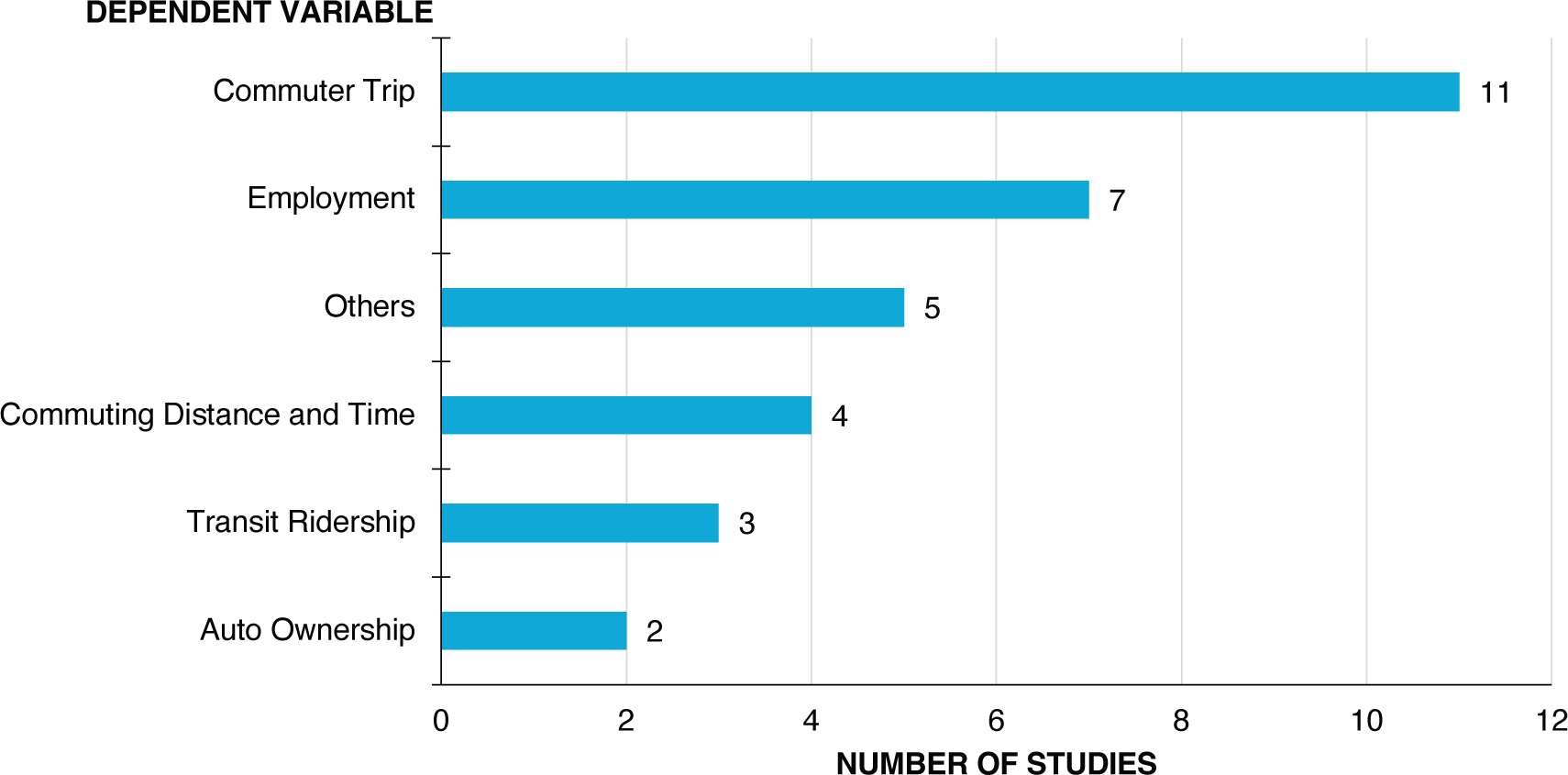
The analysis of census-related data across various topic areas has resulted in the consideration of a host of dependent variable characterizations. These include employment estimates, commute travel distance and time, auto ownership, and transit ridership. The exact formulation of the dependent variable is dependent on the study objectives and the data accessibility at the spatial resolution of interest.
A summary of the adoption of the various dependent variable characterizations across both types of studies considered in the literature review for this research is presented in Figure 8.4, which shows that the commuter trip variable is most often employed in studies using census-related data.
8.4 Research Method
The analysis of various census-related data sources and the corresponding variables of interest involves several methodological approaches. These include regression models (linear regression and linear mixed models), categorical variable analysis models for unordered variables (such as random utility approaches) and for ordered variables (such as ordered logit models), count models (negative binomial and zero-inflated negative binomial model), classification models (such as latent clustering, decision tree, random forest, gradient-boosted tree), hazard-based duration models, GIS-based accessibility measure generation, sketch modeling, and simulation.
A summary of the distribution of the various methods employed in the studies that were included in the literature review for this research is presented in Figure 8.5, which suggests that the most commonly adopted analysis methodology is regression analysis.
Long Description.
A horizontal bar chart presents the number of studies with various dependent variables. The horizontal axis shows the number of studies and ranges from 0 to 12. The vertical axis lists 6 dependent variables: Commuter Trip, Employment, Others, Commuting Distance and Time, Transit Ridership, and Auto Ownership.The dependent variable Commuter Trip was in 11 studies. Employment was in 7. Others was in 5 studies, and Commuting Distance and Time was in 4. Transit Ridership was in 3 studies, and Auto Ownership was in 2.
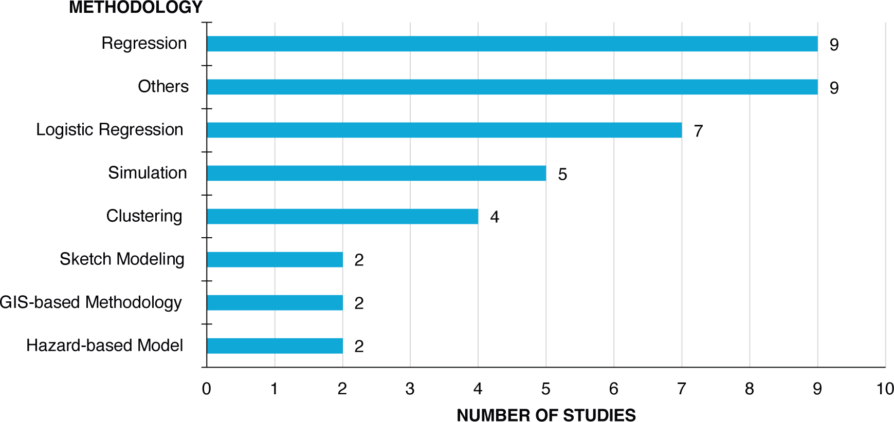
Long Description.
The horizontal bar chart displays the number of studies categorized by the methodology adopted. The horizontal axis ranges from 0 to 10, showing study count. The vertical axis lists eight methodologies: Regression, Others, Logistic Regression, Simulation, Clustering, Sketch Modeling, GIS-based Methodology, and Hazard-based Model. Regression and Others each have 9 studies. Logistic Regression has 7. Simulation has 5. Clustering has 4. Sketch Modeling, GIS-based Methodology, and Hazard-based Model each have 2 studies.


