Census Data Field Guide for Transportation Applications (2025)
Chapter: 18 Scenario: Using Public Use Microdata Sample Data to Understand Changes in Occupation Trends Due to COVID-19

CHAPTER 18
Scenario: Using Public Use Microdata Sample Data to Understand Changes in Occupation Trends Due to COVID-19
18.1 Overview
This scenario illustrates the use of PUMS to understand changes in occupation due to COVID-19. In the scenario, data from the 2019 and 2020 1-year ACS are used with experimental weights to make the comparisons meaningful.
Experimental person and household-level weights were developed to correct for the impact of the COVID-19 pandemic on the 2020 ACS data collection.
“These weights incorporate additional administrative data, including income data from the Internal Revenue Service, benefit data from the Social Security Administration, demographic data from the 2010 census, industry data for the Census Bureauʼs Business Register, and third-party home value data. These data were then incorporated into a two-stage reweighting procedure called entropy balancing. Stage one reweights respondent housing units to control for selection into response. Stage two, an estimation of individual weights to match external population totals, applies constraints to preserve the distribution of housing unit characteristics, the notion of spousal equivalence, external population targets by age, race, sex, and Hispanic origin, and to balance weights within and across months. For more information on the creation of entropy-balanced weights, the reader can review Section 5 of the working paper, Addressing Nonresponse Bias in the American Community Survey During the Pandemic Using Administrative Data” (IPUMS USA website “EXPWTH.” https://usa.ipums.org/usa-action/variables/EXPWTH#description_section).
18.2 Background
Acme Real Estate, a major real estate development company in the United States, wants to understand trends in employment changes due to their impact on the companyʼs commercial real estate holdings. Milo Yossarian, an analyst at Acme, was tasked with evaluating the changes. As a first step, Milo thought that it might be better to compare occupations within industries rather than the individual industries themselves. His reasoning for using occupation rather than industry for his analysis was that any given industry might have multiple occupations. For example, in commercial buildings, office administration personnel and engineers had job flexibility to work from home, while electricians and steel workers, who worked on the job site, did not have such an option yet and needed to be physically present at the job site to ensure that work was done properly. Therefore, Milo turned to the 2019 and 2020 PUMS data to inform his analysis of changes in occupation in the 2-year period.
18.3 Analysis
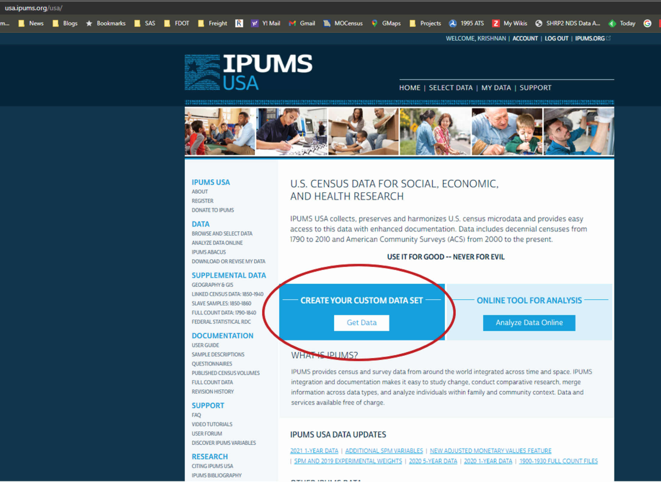
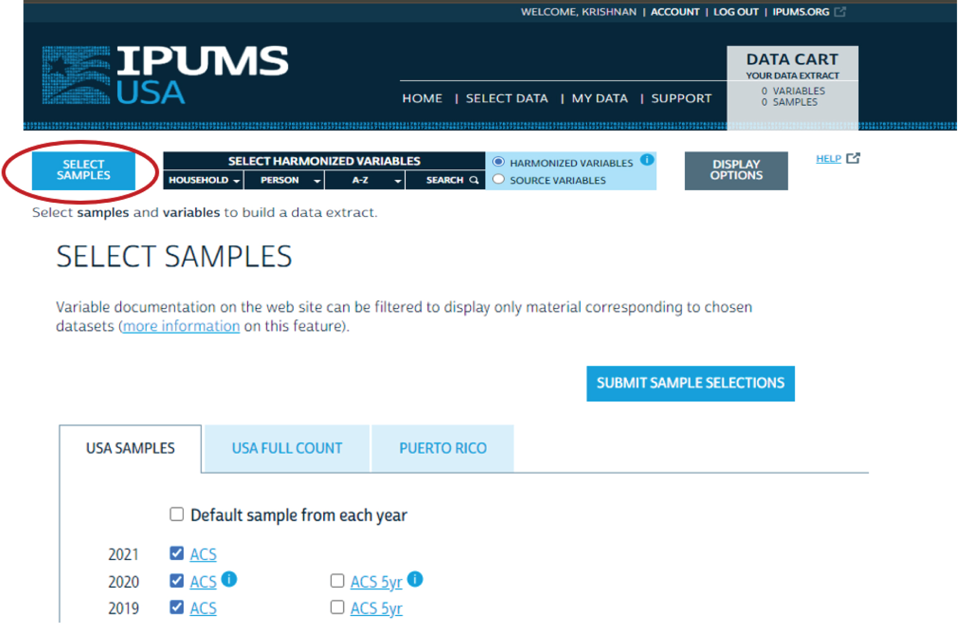
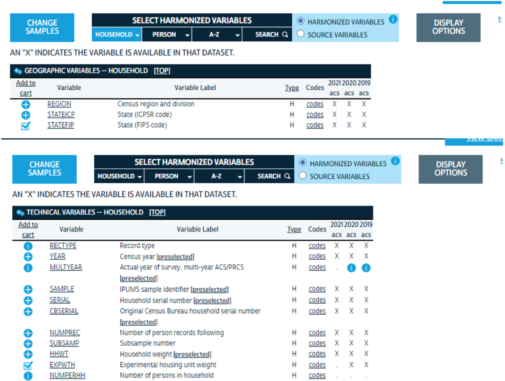
To conduct the analysis, Milo logged into his IPUMS (https://www.ipums.org/) account and created a custom dataset that contained the relevant variables. (Figure 18.1 shows the IPUMS-USA screen for creating a custom dataset.) Milo then selected samples and chose to focus on 2019, 2020, and 2021 (Figure 18.2). Once Milo had selected samples, he selected the variables that he thought were relevant for the analysis. Milo first selected variables from the household file since he wanted to understand the variability by state. He also selected household experimental weights as a variable (Figure 18.3).
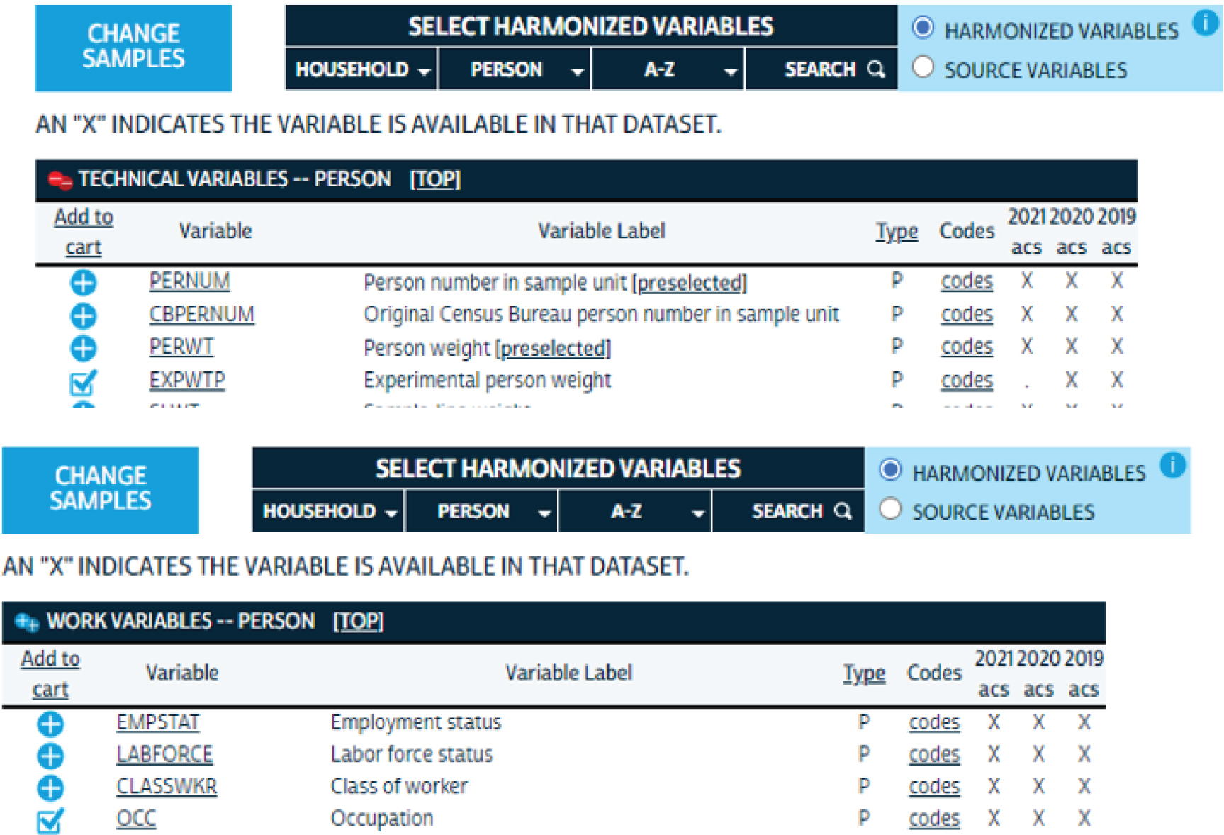
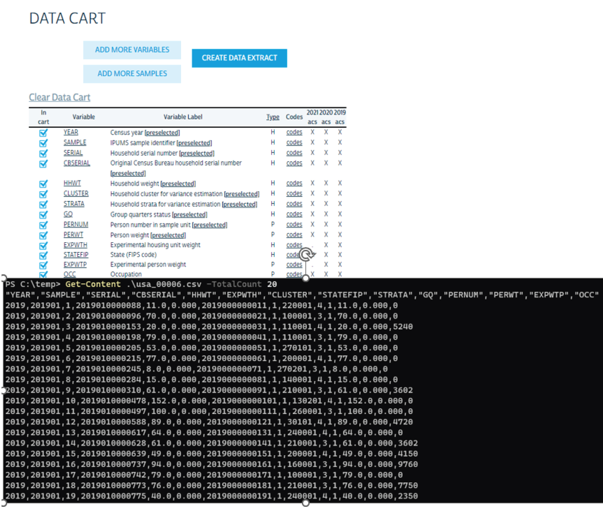
Next, he selected variables from the person file related to occupation and person experimental weights (Figure 18.4). Figure 18.5 shows the final data extract available for download, along with the first 20 rows of the data extract.
After extracting the data, Milo decided to compare different occupations to assess changes between 2019 and 2020 and to determine which occupations experienced the biggest changes.
Source: https://www.ipums.org/.
Long Description.
The screenshot shows the homepage of the IPUMSUSA website. A central, highlighted button labeled Create Your Custom Data Set, Get Data allows users to build tailored datasets. The page highlights IPUMS's support for social, economic, and health research using structured microdata from 1790 to the present. The sidebar on the left links to data selection, documentation, supplemental data, and support tools.
Source: https://www.ipums.org/.
Long Description.
The screenshot from the IPUMSUSA website highlights the Select Samples tab, allowing users to choose data samples from the American Community Survey. 2019, 2020, and 2021 ACS 1-year samples are selected. A button labeled Submit Sample Selections finalizes the choice for further customization. Tabs for USA Samples, USA Full Count, and Puerto Rico are also visible, offering dataset options by geographic coverage.
Source: https://www.ipums.org/.
Long Description.
Sections of the IPUMSUSA interface where users select harmonized household variables from the American Community Survey for 2021, 2020, and 2019. The upper panel lists geographic variables including region, state ICPSR code, and state FIPS code. State FIPS code is selected. The lower panel includes technical variables such as record type, year, sample ID, serial numbers, and weights. Each variable has availability marked with an X for the respective years, and links to view code details. Experimental housing unit weight is selected.
Source: https://www.ipums.org/.
Long Description.
Two panels from the IPUMSUSA variable selection interface. The top panel displays technical person variables such as person number in household, Census Bureau person number, person weight, and experimental person weight. Experimental person weight is selected. The lower panel lists work-related person variables including employment status, labor force status, class of worker, and occupation. Occupation is selected. Availability for the American Community Survey is marked with Xs across 2021, 2020, and 2019, and variable-specific code links are provided for further details.
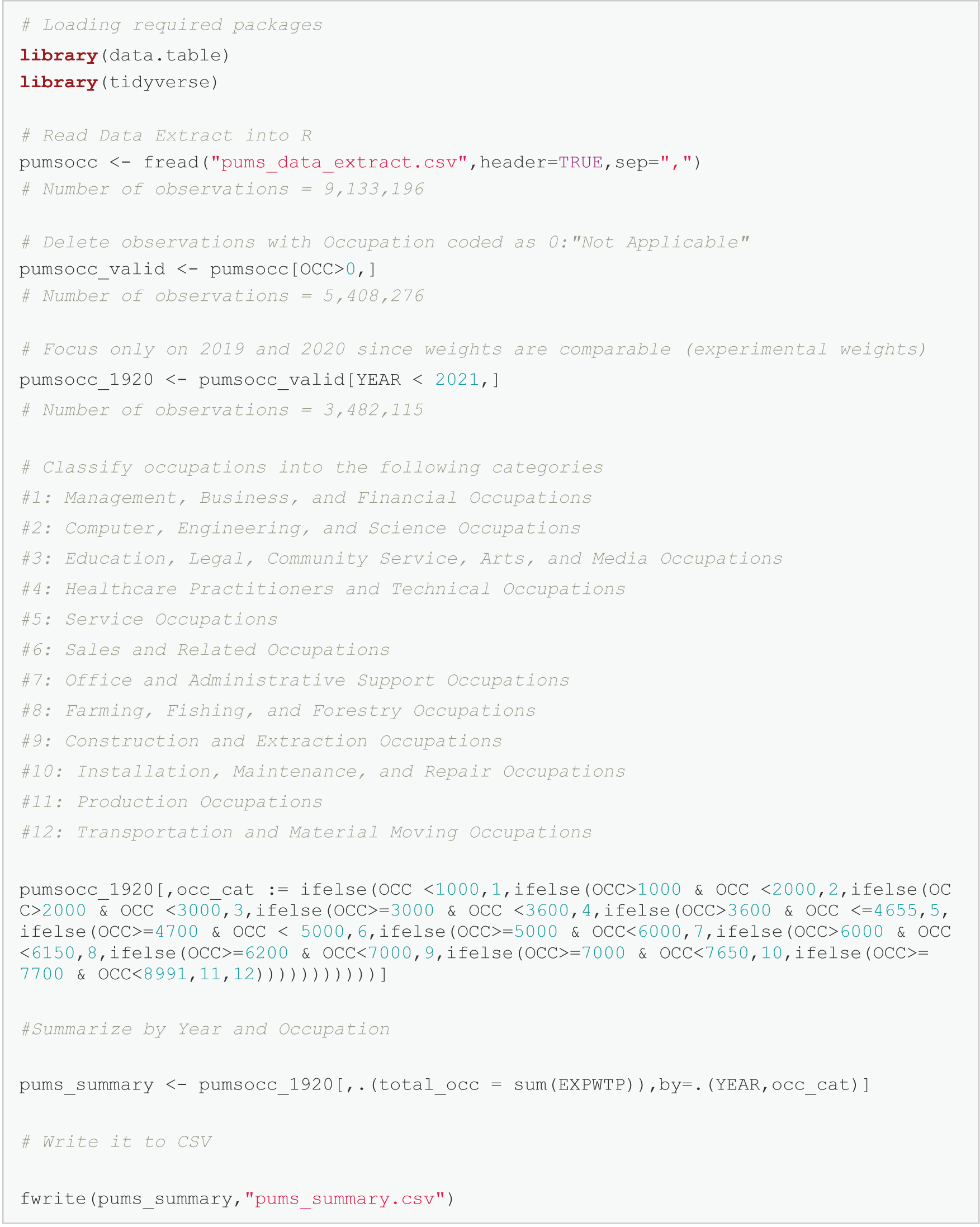
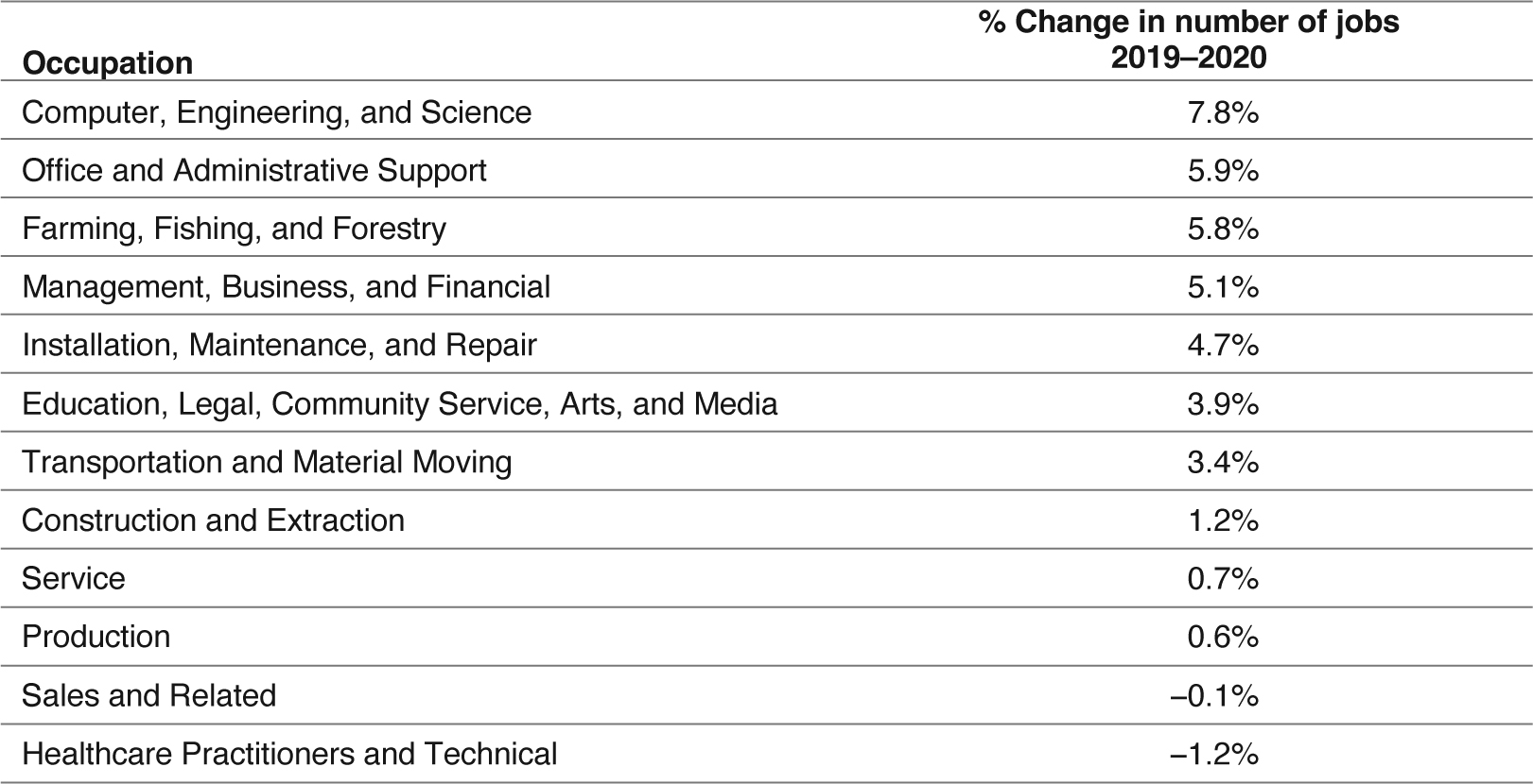
Since there were 530 different occupations, Milo organized them into 12 categories to make the comparisons more meaningful. Figure 18.6 shows the R code that was used to obtain the PUMS data and to group them into the 12 categories. Table 18.1 shows the results of the analysis. While most occupations saw an increase in the number of jobs, the “sales and related” category and the “healthcare practitioners and technical” category lost jobs during this time period, which included the height of the COVID-19 pandemic in 2020. Jobs in production, service, and construction and extraction also showed weaker growth during the same time period.
Given the importance of location in determining real estate decisions, Milo decided to compare the occupational changes between 2019 and 2020 at the state level. While Milo would have preferred more granular PUMS spatial data, this was not feasible given the nature of the PUMS and the PUMA.
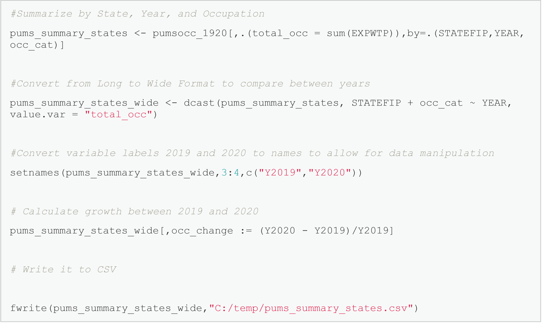
Figure 18.7 shows a continuation of the code shown in Figure 18.6, and the results of the analysis are shown in Table 18.2. Where Table 18.1 shows changes in number of jobs by occupation at the national level, Table 18.2 shows changes in number of jobs by occupation at the state level.
In general, Table 18.2 shows variability in patterns of job growth and job loss patterns across states. Nonetheless, reflecting the overall drop in jobs at the national level, jobs in the healthcare practitioners and technical category decreased across 31 of the 50 states and the District of Columbia, while jobs in the sales and related category decreased in 29 states.
In sectors that exhibited weak job growth at a national level, there was also quite a bit of variability across states. Production jobs decreased in 25 states, service jobs decreased in 21 states, and construction and extraction jobs decreased in 16 states.
Source: https://www.ipums.org/.
Long Description.
The interface shows two panels. The top panel is the IPUMSUSA Data Cart interface listing selected variables across ACS samples from 2019 to 2021, including household identifiers such as: IPUMS sample identifier (SAMPLE), household serial number (SERIAL), and original census bureau household serial number (CBSERIAL); weights such as household weight (HHWT), person weight (PERWT), and experimental housing unit weight (EXPWTP); geographic codes such as state FIPS code (STATE FIP), household cluster for variance estimation (CLUSTER), household strata for variance estimation (STRATA); and person-level variables such as group quarters status (GQ), person number (PERNUM), and occupation (OCC). The bottom panel shows a Power Shell terminal displaying the first 20 rows of a downloaded comma-separated values file named u s a underscore 0 0 0 0 6 dot csv, confirming successful export and structure of the dataset.
Note: An electronic version of the R code used in the scenarios described in this report is available on the National Academies Press website (nap.nationalacademies.org) in the Resources section of the catalog page for NCHRP Research Report 1108: Census Data Field Guide for Transportation Applications.
Long Description.
# Loading required packages
library(data.table)
library(tidyverse)
# Read Data Extract into R
p u m s o c c <- f read("p u m s_data_extract.c s v",header=TRUE,sep=",")
# Number of observations = 9,133,196
# Delete observations with Occupation coded as 0:"Not Applicable"
p u m s o c c_valid <- p u m s o c c[O C C>0,]
# Number of observations = 5,408,276
# Focus only on 2019 and 2020 since weights are comparable (experimental weights)
p u m s o c c_1920 <- p u m s o c c_valid[YEAR < 2021,]
# Number of observations = 3,482,115
# Classify occupations into the following categories
#1: Management, Business, and Financial Occupations
#2: Computer, Engineering, and Science Occupations
#3: Education, Legal, Community Service, Arts, and Media Occupations
#4: Healthcare Practitioners and Technical Occupations
#5: Service Occupations
#6: Sales and Related Occupations
#7: Office and Administrative Support Occupations
#8: Farming, Fishing, and Forestry Occupations
#9: Construction and Extraction Occupations
#10: Installation, Maintenance, and Repair Occupations
#11: Production Occupations
#12: Transportation and Material Moving Occupations
p u m s o c c_1920[,o c c_cat := ifelse(O C C <1000,1,ifelse(O C C>1000 & O C C <2000,2,ifelse(O C C>2000 & O C C <3000,3,ifelse(O C C>=3000 & O C C <3600,4,ifelse(O C C>3600 & O C C <=4655,5,ifelse(O C C>=4700 & O C C < 5000,6,ifelse(O C C>=5000 & O C C <6000,7,ifelse(O C C>6000 & O C C <6150,8,ifelse(O C C>=6200 & O C C <7000,9,ifelse(O C C>=7000 & O C C <7650,10,ifelse(O C C>=7700 & O C C <8991,11,12)))))))))))]
#Summarize by Year and Occupation
p u m s_summary <- p u m s o c c_1920[,.(total_o c c = sum(EXPWTP)),by=.(YEAR,o c c_cat)]
# Write it to CSV
f write(p u m s_summary,"p u m s_summary.c s v")
Long Description.
The table has 2 columns and 12 rows. The column headers read occupation and percentage change in the number of jobs from 2019 to 2020. The row details are as follows. Row 1: Computer, engineering, and science; 7.8 percent. Row 2: Office and administrative support, 5.9 percent. Row 3: Farming, fishing, and forestry, 5.8 percent. Row 4: Management, business, and financial, 5.1 percent. Row 5: Installation, maintenance, and repair, 4.7 percent. Row 6: Education, legal, community service, arts, and media, 3.9 percent. Row 7: Transportation and material moving, 3.4 percent. Row 8: Construction and extraction, 1.2 percent. Row 9: Service, 0.7 percent. Row 10: Production, 0.6 percent. Row 11: Sales and related, negative 0.1 percent. Row 12: Healthcare practitioners and technical, negative 1.2 percent.
Note: An electronic version of the R code used in the scenarios described in this report is available on the National Academies Press website (nap.nationalacademies.org) in the Resources section of the catalog page for NCHRP Research Report 1108: Census Data Field Guide for Transportation Applications.
Long Description.
#Summarize by State, Year, and Occupation
p u m s_summary_states <- p u m s o c c_1920[,.(total_o c c = sum(EXPWTP)),by=.(STATEFIP,YEAR,o c c_cat)]
#Convert from Long to Wide Format to compare between years
p u m s_summary_states_wide <- d cast(p u m s_summary_states, STATEFIP + o c c_cat ~ YEAR, value.v a r = "total_o c c")
#Convert variable labels 2019 and 2020 to names to allow for data manipulation
setnames(p u m s_summary_states_wide,3:4,c("Y2019","Y2020"))
# Calculate growth between 2019 and 2020
p u m s_summary_states_wide[,o c c_change := (Y2020 - Y2019)/Y2019]
# Write it to CSV
f write(p u m s_summary_states_wide,"C:/temp/p u m s_summary_states.c s v")

Long Description.
The table has 13 columns and 50 rows. The columns are the following: state; computer, engineering, and science; construction and extraction; education, legal, community service, arts, and media; farming, fishing, and forestry; healthcare practitioners and technical; installation, maintenance, and repair; management, business, and financial; office and administrative support; production; sales and related; service; and transportation and material moving. Negative values are highlighted. Row details are as follows. Row 1: Alabama, 11.2%, 1.3%, 2.5%, 46.1%, 0.7%, 8.9%, 2.0%, 6.9%,−2.7%, −2.2%, 1.8%, -4.1%. Row 2: Alaska, 7.3%, 19.4%, −13.8%, 57.6%, 20.3%, −0.1%, 16.0%, −11.3%, 14.2%, −17.0%, 13.1%, 10.5%. Row 3: Arizona, 7.8%, −4.4%, 7.5%, −0.3%, 1.3%, 4.9%, 7.6%, 7.0%, 8.4%, 5.1%, 0.7%, 3.6%. Row 4: Arkansas, 34.5%, 8.5%, −5.3%, −0.3%, 12.3%, 11.6%, 5.8%, 7.6%, −4.0%, −0.3%, −0.9%, -4.0%. Row 5: California, 7.6%, -3.4%, 4.3%, -1.6%, -3.2%, 6.6%, 3.8%, 5.7%, 2.5%, -3.6%, 1.1%, 2.8%. Row 6: Colorado, 3.0%, 3.3%, 3.4%, 4.1%, 1.5%, 20.2%, 1.1%, 4.2%, -3.7%, 3.1%, -0.9%, 13.8%. Row 7: Connecticut, 2.4%, 5.8%, 3.0%, 40.5%, -1.0%, 5.6%, 4.1%, 9.2%, 14.6%, -0.1%, -5.5%, 6.3%. Row 8: Delaware, 9.6%, 19.1%, 13.6%, -32.6%, -21.6%, 0.5%, -3.6%, -2.1%, 19.4%, 16.5%, 12.4%, 15.6%. Row 9: Florida, 9.7%, 4.6%, 3.1%, -24.9%, -1.7%, 8.1%, 7.6%, 7.1%, -0.8%, 2.4%, -0.5%, 5.5%. Row 10: Georgia, 12.1%, 5.2%, 0.5%, 6.1%, 3.3%, -6.4%, 6.5%, 6.7%, 1.0%, 1.4%, 2.3%, 0.1%. Row 11: Hawaii, 9.8%, -5.2%, 9.8%, -4.9%, -5.2%, -6.9%, 0.9%, 4.7%, -6.1%, -3.6%, 5.0%, 26.0%. Row 12: Idaho, 24.9%, 16.8%, 0.8%, 22.1%, 12.9%, 22.9%, 8.3%, -8.1%, -7.0%, -9.2%, 7.8%, 8.0%. Row 13: Illinois, -1.4%, -1.3%, 4.8%, 19.8%, -4.2%, 5.6%, 2.9%, 1.9%, 1.1%, -0.8%, -2.0%, 8.4%. Row 14: Indiana, -0.1%, 5.6%, 6.9%, 0.4%, 6.5%, 0.3%, 8.9%, 5.1%, -2.2%, -0.4%, -2.7%, 3.4%. Row 15: Iowa, −3.2%, 6.0%, 0.4%, 11.9%, 6.7%, −1.9%, 5.4%, 3.4%, 9.4%, −0.4%, 2.2%, −2.4%. Row 16: Kansas, 7.3%, 4.9%, 6.2%, 34.1%, −2.7%, 1.6%, 1.9%, 10.4%, −5.5%, −0.3%, 5.4%, −0.5%. Row 17: Kentucky, 1.8%, 0.8%, 0.4%, 6.6%, −5.6%, 3.3%, 0.9%,10.3%, −3.8%, 4.2%, 8.8%, 9.2%. Row 18: Louisiana, 8.1%, 8.3%, 8.4%, −19.4%, −3.4%, −5.8%, 0.5%, 10.1%, −1.7%, 2.7%, −3.0%, 2.4%. Row 19: Maine, −10.7%, 23.2%, 0.3%, 2.1%, −4.4%, −1.1%, 2.6%, 5.1%, 1.8%, 2.7%, −4.3%, 10.7%. Row 20: Maryland, 5.6%, 2.1%, −2.4%, 9.2%, −5.6%, −0.9%, 8.5%, 3.8%, −4.8%, 1.8%, −4.3%, 0.7%. Row 21: Massachusetts, 7.5%, −8.4%, 3.3%, 29.5%, 1.3%, 9.9%, 4.7%, 8.2%, −0.4%, 2.6%, −1.0%, 6.9%. Row 22: Michigan, 9.7%, 2.9%, 6.9%, −14.2%, −1.9%, −1.4%, 4.1%, 7.7%, −1.8%, −1.1%, 3.4%, 3.1%. Row 23: Minnesota, 2.5%, 10.1%, 2.1%, 30.4%, −3.7%, 11.3%, 7.8%, −1.9%, −0.9%, −6.8%, 0.3%, 3.0%. Row 24: Mississippi, 5.4%, 9.6%, 12.2%, 1.4%, −3.0%, 0.0%, 0.2%, 1.5%, 2.5%, −3.5%, 1.3%, −0.9%. Row 25: Missouri, 5.3%, 0.9%, 5.2%, 35.4%, −10.2%, 6.9%, 6.3%, −1.2%, 1.2%, −0.8%, 3.7%, 0.4%. Row 26: Montana, −11.2%, 14.0%, −4.5%, −4.3%, −14.4%, 24.1%, 13.1%, 14.0%, 4.9%, −20.1%, −0.6%, 13.1%. Row 27: Nebraska, 24.3%, −7.5%, 6.5%, 0.8%, −7.5%, 10.2%, 6.4%, 1.5%, 1.0%, −9.8%, −11.0%, 3.9%. Row 28: Nevada, 46.7%, 0.2%, 6.3%, −34.1%, 12.5%, 5.3%, 3.3%, 10.3%, 0.4%, 1.5%, −2.3%, −7.4%. Row 29: New Hampshire, 6.7%, 19.8%, −3.6%, −2.6%, 0.0%, 8.2%, 6.8%, 0.9%, 1.5%, −4.0%, 10.4%, −11.8%. Row 30: New Jersey, 2.6%, −7.1%, 9.3%, −8.4%, 1.9%, −0.2%, 1.9%, −1.2%, 8.0%, 2.4%, −0.8%, 2.8%. Row 31: New Mexico, 4.1%, 11.3%, 1.9%, −17.4%, −4.7%, 3.0%, 2.3%, 9.7%, 9.1%, 7.7%, −2.9%, 6.5%. Row 32: New York, 8.8%, 1.0%, 2.6%, 21.8%, −3.5%, 2.4%, 0.6%, 11.1%, 1.6%, −0.6%, −3.4%, 4.0%. Row 33: North Carolina, 11.8%, −6.8%, 5.5%, 36.7%, −0.6%, −0.4%, 6.8%, 11.8%, −4.9%, 2.9%, 1.1%, 7.1%. Row 34: North Dakota, 15.0%, −21.4%, 8.5%, 10.8%, −9.0%, −4.3%, 3.2%, −0.3%, 7.4%, −9.6%, 12.1%, −9.9%. Row 35: Ohio, 9.5%, 7.0%, 3.9%, −8.6%, −0.7%, 4.7%, 1.5%, 5.7%, −2.1%, −2.2%, 2.6%, 5.7%. Row 36: Oklahoma, 14.7%, 5.9%, 9.0%, −3.7%, −3.5%, 9.2%, 2.7%, 9.6%, −2.5%, 0.9%, 1.7%, −1.3%. Row 37: Oregon, 8.1%, 7.9%, −2.7%, 8.9%, −0.1%, 12.8%, 11.5%, 5.2%, −2.1%, −0.3%, −2.5%, −4.0%. Row 38: Pennsylvania, 5.7%, 8.0%, 6.1%, 11.7%, −4.8%, −4.1%, 6.6%, −0.6%, 4.0%, 1.8%, 6.0%, −2.4%. Row 39: Rhode Island, 1.3%, 13.6%, −0.6%, 79.7%, −6.5%, 14.5%, 5.6%, 12.4%, −12.2%, 11.7%, 3.3%, 14.0%. Row 40: South Carolina, 11.0%, 9.4%, 13.3%, −6.0%, 6.7%, 1.0%, −4.5%, 9.3%, −6.6%, 4.9%, −0.9%, 10.7%. Row 41: South Dakota, −0.8%, −0.7%, −7.5%, 83.0%, 9.5%, 71.6%, −0.1%, 3.2%, −3.5%, −4.6%, 4.4%, 21.2%. Row 42: Tennessee, 14.8%, 6.4%, 5.1%, 20.7%, 2.8%, −5.6%, 7.4%, 7.7%, 1.0%, −5.3%, 2.1%, 9.0%. Row 43: Texas, 10.6%, −3.9%, 3.1%, 5.8%, 1.1%, 11.9%, 9.3%, 10.4%, 2.2%, −0.1%, 2.1%, 2.4%. Row 44: Utah, 18.0%, −7.4%, 1.9%, 39.4%, 3.0%, 5.6%, 0.5%, 12.4%, 5.2%, 7.7%, 2.4%, 0.6%. Row 45: Vermont, −1.6%, 5.8%, 7.3%, −16.4%, −9.3%, 17.7%, −0.3%, 17.1%, −4.5%, −10.9%, 9.0%, 19.8%. Row 46: Virginia, 6.5%, −1.2%, 3.2%, −16.6%, −8.5%, 4.7%, 12.0%, −0.5%, −3.2%, 1.5%, 4.0%, 4.5%. Row 47: Washington, 8.9%, 3.1%, 4.7%, 24.0%, 1.7%, −0.2%, 6.3%, 1.9%, 3.1%, 4.1%, −2.8%, 1.7%. Row 48: West Virginia, 0.4%, −11.2%, 12.7%, −19.0%, −4.5%, 1.4%, 12.2%, 3.4%, −1.3%, −5.1%, −5.0%, 10.3%. Row 49: Wisconsin, 8.2%, −0.7%, −0.9%, 27.1%, 7.8%, 9.0%, 5.9%, 3.4%, 8.3%, −2.5%, 0.2%, −2.4%. Row 50: Wyoming, −13.9%, −23.5%, −8.6%, 58.6%, 4.8%, 41.6%, 15.6%, 3.1%, 27.0%, −2.7%, −5.1%, 13.3%.


