Census Data Field Guide for Transportation Applications (2025)
Chapter: 15 Scenario: Statewide Snapshot of Mean Travel Times

CHAPTER 15
Scenario: Statewide Snapshot of Mean Travel Times
15.1 Overview
This scenario, like the scenario presented in Chapter 14, shows how to download a CTPP table relevant to a particular inquiry and modify the table using R to provide insights into the data.
15.2 Background
Jenny Modeler is a member of the Forecasting and Trends Office at a large state transportation agency, and her supervisor has requested that Jenny provide a county-level estimate of average travel times for commuters.
15.3 Analysis
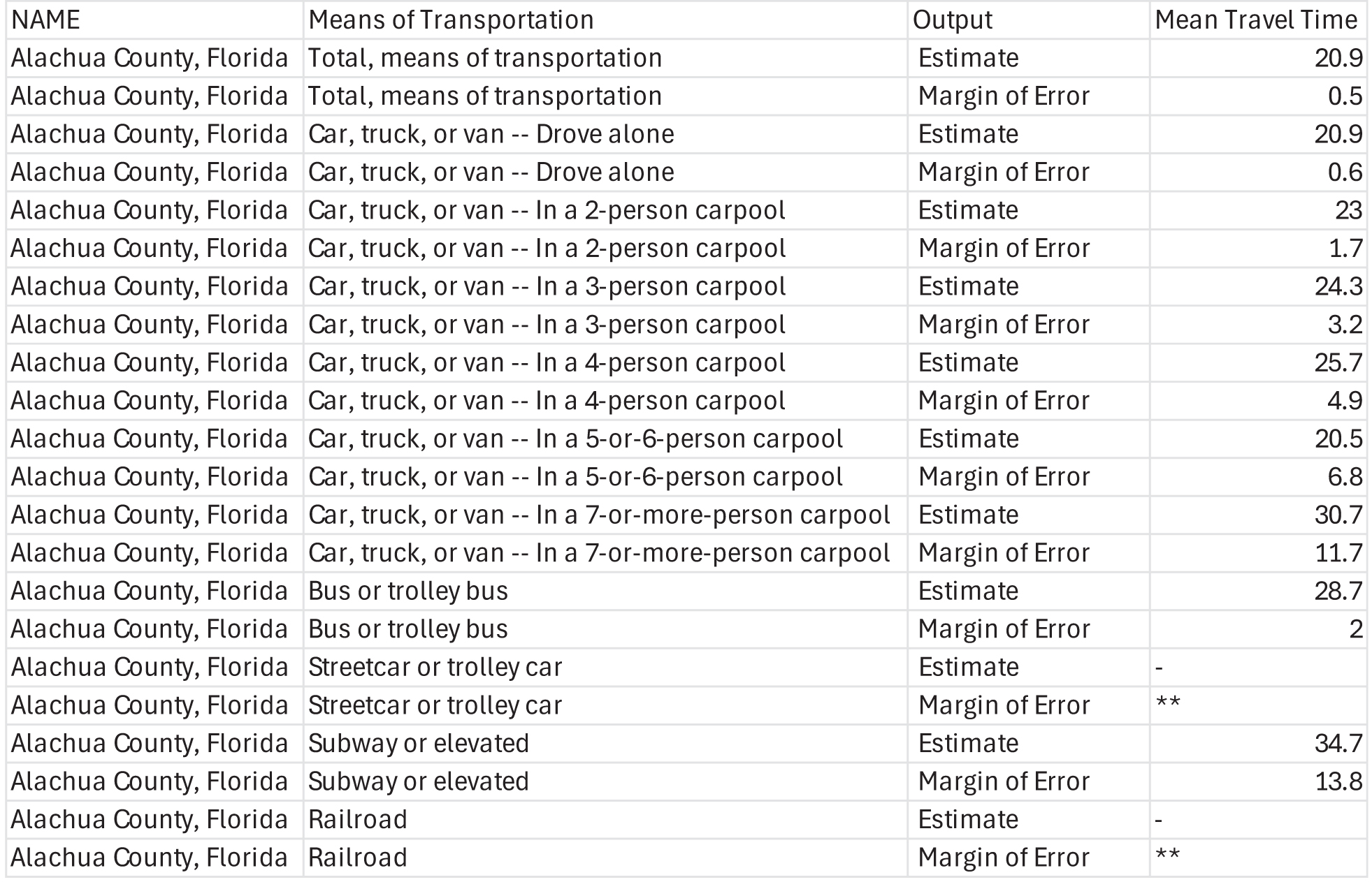
Jenny accesses the ACTS program website, creates a new selection set showing only the stateʼs counties, and downloads Table B106202—Mean Travel time (1) by Means of transportation (18) (Workers 16 years and over who did not work at home). The resulting dataset is shown in Figure 15.1.
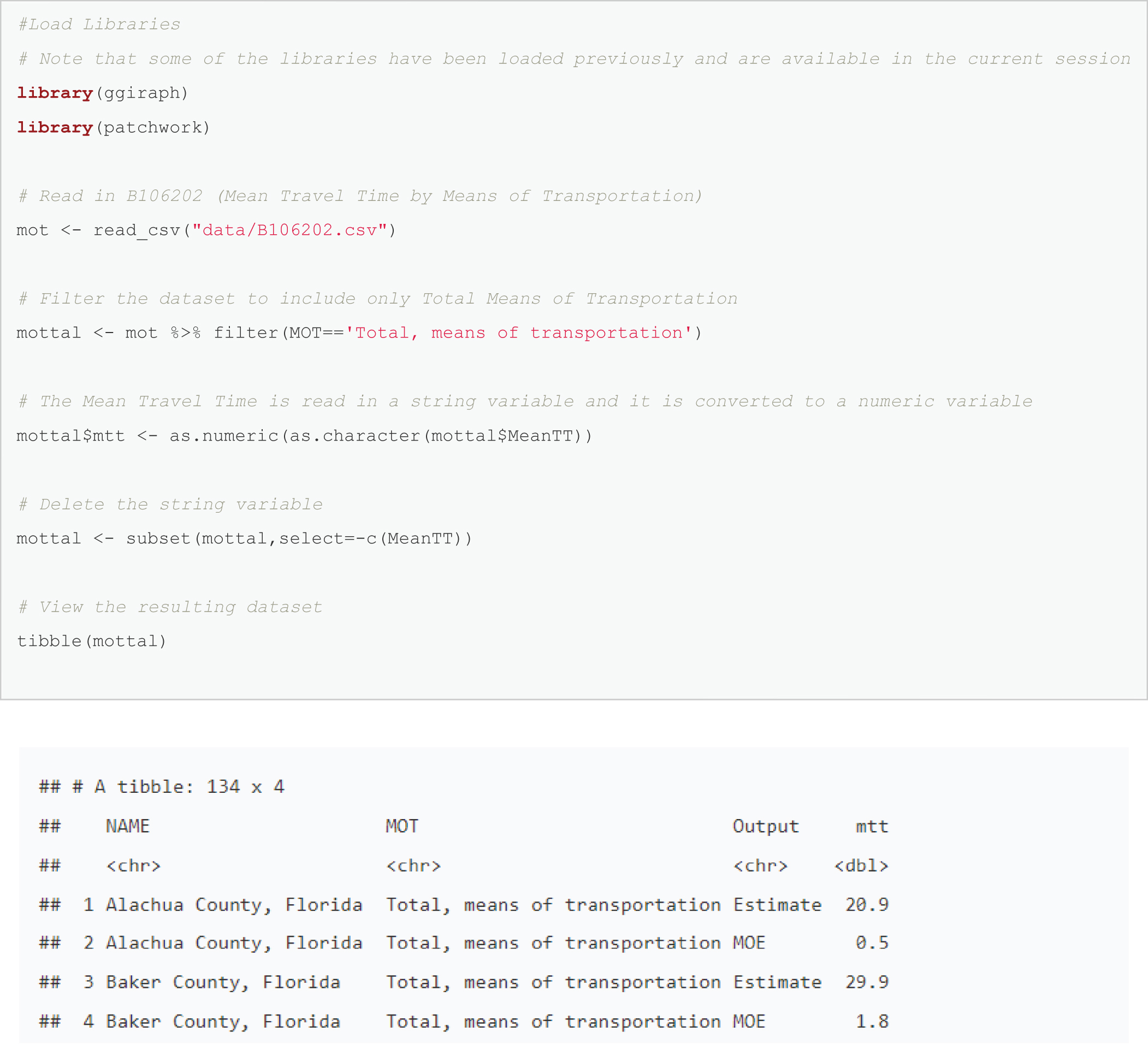
To start, the data needs to be restructured and county geometry needs to be attached to the data. The steps that Jenny undertakes are shown in the code chunk presented in Figure 15.2.
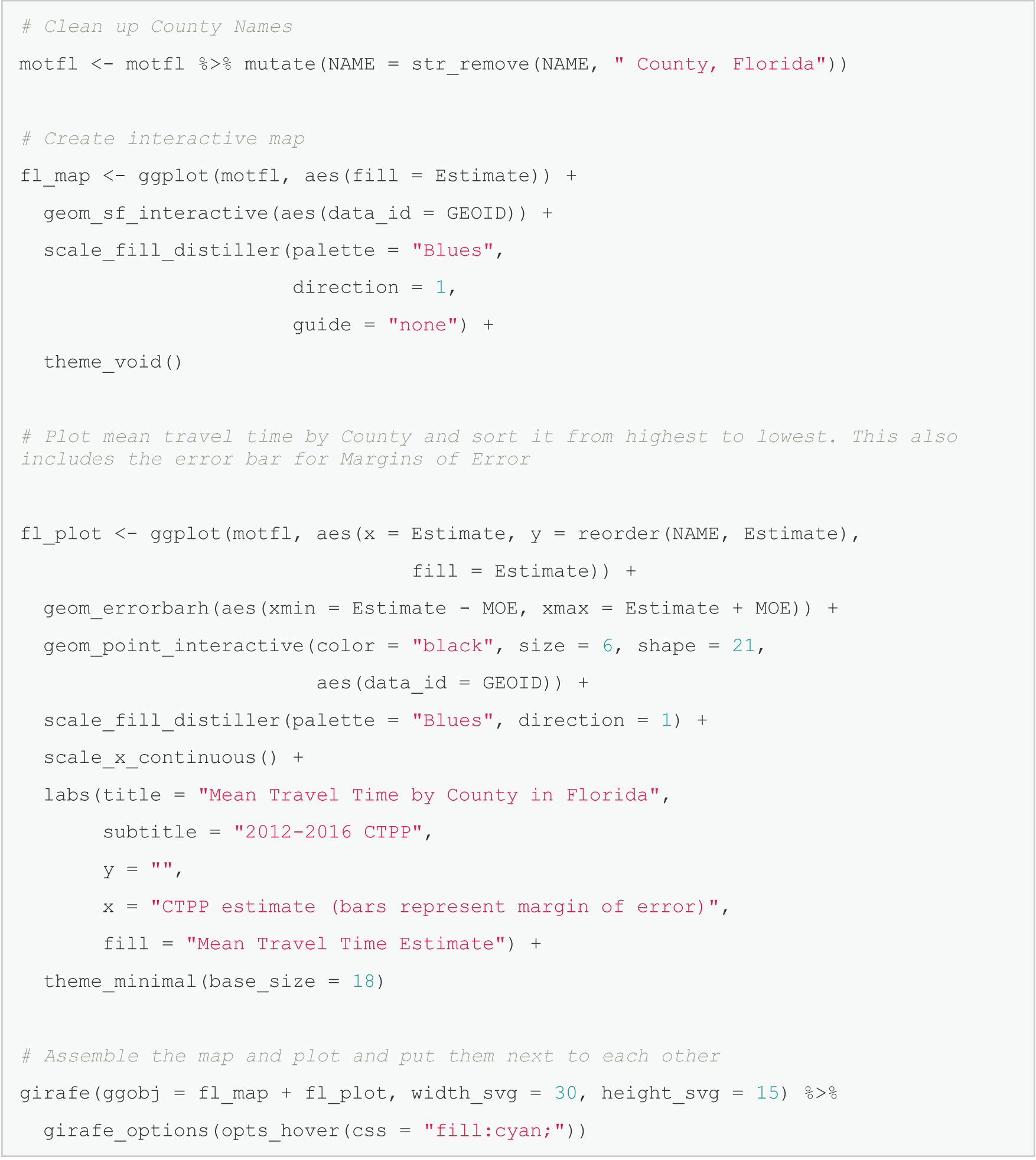
Once Jenny has cleaned up the dataset, it is ready for visualization, as requested by her supervisor. The visual representation of mean travel times by county that Jenny provides allows a user to click on a county and identify total average travel time (Figure 15.3 and Figure 15.4). The R code to create the interactive map was adapted from Analyzing U.S. Census Data: Methods, Maps, and Models in R (Walker n.d.).
Source: ACTS.
Long Description.
The table has 4 columns and 22 rows. The column headers include Name, Means of Transportation, Output, and Mean Travel Time. Row 1: Alachua County, Florida; Total means of transportation; Estimate; 20.9. Row 2: Alachua County, Florida; Total means of transportation; Margin of Error; 0.5. Row 3: Alachua County, Florida; Car, truck, or van, drove alone; Estimate; 20.9. Row 4: Alachua County, Florida; Car, truck, or van, drove alone; Margin of Error; 0.6. Row 5: Alachua County, Florida; Car, truck, or van in a 2-person carpool; Estimate; 23. Row 6: Alachua County, Florida, Car, truck, or van in a 2-person carpool; Margin of Error; 1.7. Row 7: Alachua County, Florida; Car, truck, or van in a 3-person carpool; Estimate; 24.3. Row 8: Alachua County, Florida; Car, truck, or van in a 3-person carpool; Margin of Error; 3.2. Row 9: Alachua County, Florida; Car, truck, or van in a 4-person carpool; Estimate; 25.7. Row 10: Alachua County, Florida; Car, truck, or van in a 4-person carpool; Margin of Error; 4.9. Row 11: Alachua County, Florida; Car, truck, or van in a 5- or 6-person carpool; Estimate; 20.5. Row 12: Alachua County, Florida; Car, truck, or van in a 5- or 6-person carpool; Margin of Error; 6.8. Row 13: Alachua County, Florida; Car, truck, or van in a 7-or-more-person carpool; Estimate; 30.7. Row 14: Alachua County, Florida; Car, truck, or van in a 7-or-more-person carpool; Margin of Error; 11.7. Row 15: Alachua County, Florida; Bus or trolley bus; Estimate; 28.7. Row 16: Alachua County, Florida; Bus or trolley bus; Margin of Error; 2. Row 17: Alachua County, Florida; Streetcar or trolley car; Estimate; dash. Row 18: Alachua County, Florida; Streetcar or trolley car; Margin of Error; double star. Row 19: Alachua County, Florida; Subway or elevated; Estimate; 34.7. Row 20: Alachua County, Florida; Subway or elevated; Margin of Error; 13.8. Row 21: Alachua County, Florida; Railroad; Estimate; dash. Row 22: Alachua County, Florida; Railroad; Margin of Error; double star.
Note: An electronic version of the R code used in the scenarios described in this report is available on the National Academies Press website (nap.nationalacademies.org) in the Resources section of the catalog page for NCHRP Research Report 1108: Census Data Field Guide for Transportation Applications.
Long Description.
There are three chunks of R code. Each is followed by a dataset. The first chunk of R code is as follows:
#Load Libraries
# Note that some of the libraries have been loaded previously and are available in the current session
library(g giraph)
library(patchwork)
# Read in B106202 (Mean Travel Time by Means of Transportation)
m o t <- read_c s v("data/B106202.c s v")
# Filter the dataset to include only Total Means of Transportation
mottal <- m o t %>% filter(MOT=='Total, means of transportation')
# The Mean Travel Time is read in a string variable and it is converted to a numeric variable
mottal$m t t <- a s.numeric(a s.character(mottal$Mean T T))
# Delete the string variable
mottal <- subset(mottal,select=-c(Mean T T))
# View the resulting dataset
tibble(mottal).
In the dataset that follows, there is text at the top that reads A tibble: 134 x 4. Material follows in tabular format with five columns: a number; NAME; MOT; Output; and m t t. The first row under the colum heads is unnumbered but shows <c h r > under NAME, MOT and Output and <d b l > under m t t. The next row shows 1; Alachua County, Florida; Total, means of transportation; Estimate; 20.9 The next row shows 2; Alachua County, Florida; Total, means of transportation; MOE; 0.5. The next row shows 3; Baker County, Florida; Total, means of transportation; Estimate; 29.9. The final row shows 4; Baker County, Florida; Total, means of transportation; MOE; 1.8.
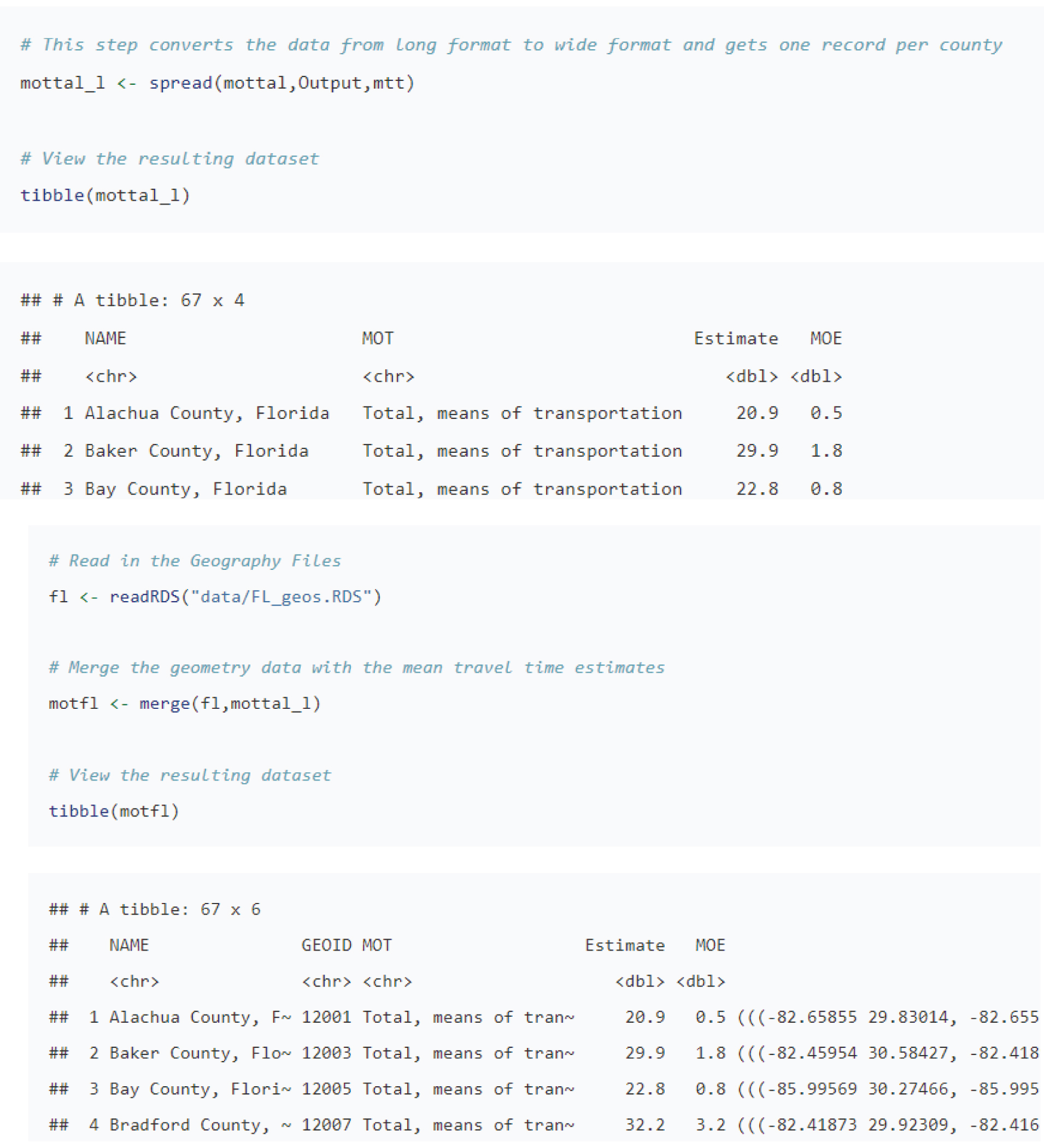
The second chunk of R code is the following:
# This step converts the data from long format to wide format and gets one record per county
mottal_l <- spread(mottal,Output,m t t)
# View the resulting dataset
tibble(mottal_l)
In the dataset that follows, text at the top reads A tibble: 67 x 4. Material in tabular format follows with five columns: number; NAME; MOT; Estimate; and MOE . The first row under the column heads is unnumbered and shows <c h r > under NAME and MOT and <d b l > under estimate and MOE. The second row shows 1, Alachua County, Florida; Total, means of transportation; 20.9; 0.5. The third row shows 2; Baker County, Florida; Total, means of transportation; 29.9; 1.8. The fourth row shows 3; Bay County Forida; Total, means of transportation; 22.8; 0.8.
The third chunk of R code is the following:
# Read in the Geography Files
f l <- readR D S("data/F L_geos.R D S")
# Merge the geometry data with the mean travel time estimates
motfl <- merge(f l,mottal_l)
# View the resulting dataset
tibble(motfl)
In the dataset that follows, text at the top reads A tibble: 67 x 6. Material is in tabular format with seven columns: number or blank; NAME; GEOID; MOT; Estimate; MOE; and and a final, unnamed column. The first row under the column heads is unnumbered and shows <c h r > under NAME, GEOID, and MOT and <d b l > under Estimate and MOE. The second row shows 1, Alachua County, Florida; 12001; Total, means of transportation; 20.9; 0.5; (((- 82.65855 29.83014, -82.655. Third row shows 2; Baker County, Florida; 12003; Total, means of transportation; 29.9; 1.8; (((-82.45954 30.58427, -82.418. The fourth row shows 3; Bay County, Florida; 12005; Total, means of transportation; 22.8; 0.8; (((-85.99569 30.27466, -85.995. The final row shows 4; Bradford County, Florida; 12007; Total, means of transportation; 32.2; 3.2; (((-82.41873 29.92309, -82.416.
Note: An electronic version of the R code used in the scenarios described in this report is available on the National Academies Press website (nap.nationalacademies.org) in the Resources section of the catalog page for NCHRP Research Report 1108: Census Data Field Guide for Transportation Applications.
Long Description.
# Clean up County Names
m o t f l <- m o t f l %>% mutate(NAME = s t r_remove(NAME, " County, Florida"))
# Create interactive map
f l_map <- g g plot(m o t f l, a e s(fill = Estimate)) +
g e o m_s f_interactive(a e s(data_i d = GEOID)) +
scale_fill_distiller(palette = "Blues",
direction = 1,
guide = "none") +
theme_void()
# Plot mean travel time by County and sort it from highest to lowest. This also includes the error bar for Margins of Error
f l_plot <- g g plot(m o t f l, a e s(x = Estimate, y = reorder(NAME, Estimate),
fill = Estimate)) +
g e o m_errorbar h(a e s(xmin = Estimate - MOE, xmax = Estimate + MOE)) +
g e o m_point_interactive(color = "black", size = 6, shape = 21,
a e s(data_i d = GEOID)) +
scale_fill_distiller(palette = "Blues", direction = 1) +
scale_x_continuous() +
labs(title = "Mean Travel Time by County in Florida",
subtitle = "2012-2016 C T P P",
y = "",
x = "C T P P estimate (bars represent margin of error)",
fill = "Mean Travel Time Estimate") +
theme_minimal(base_size = 18)
# Assemble the map and plot and put them next to each other
girafe(g g o b j = f l_map + f l_plot, width_s v g = 30, height_s v g = 15) %>%
girafe_options(opts_hover(c s s = "fill:cyan;"))
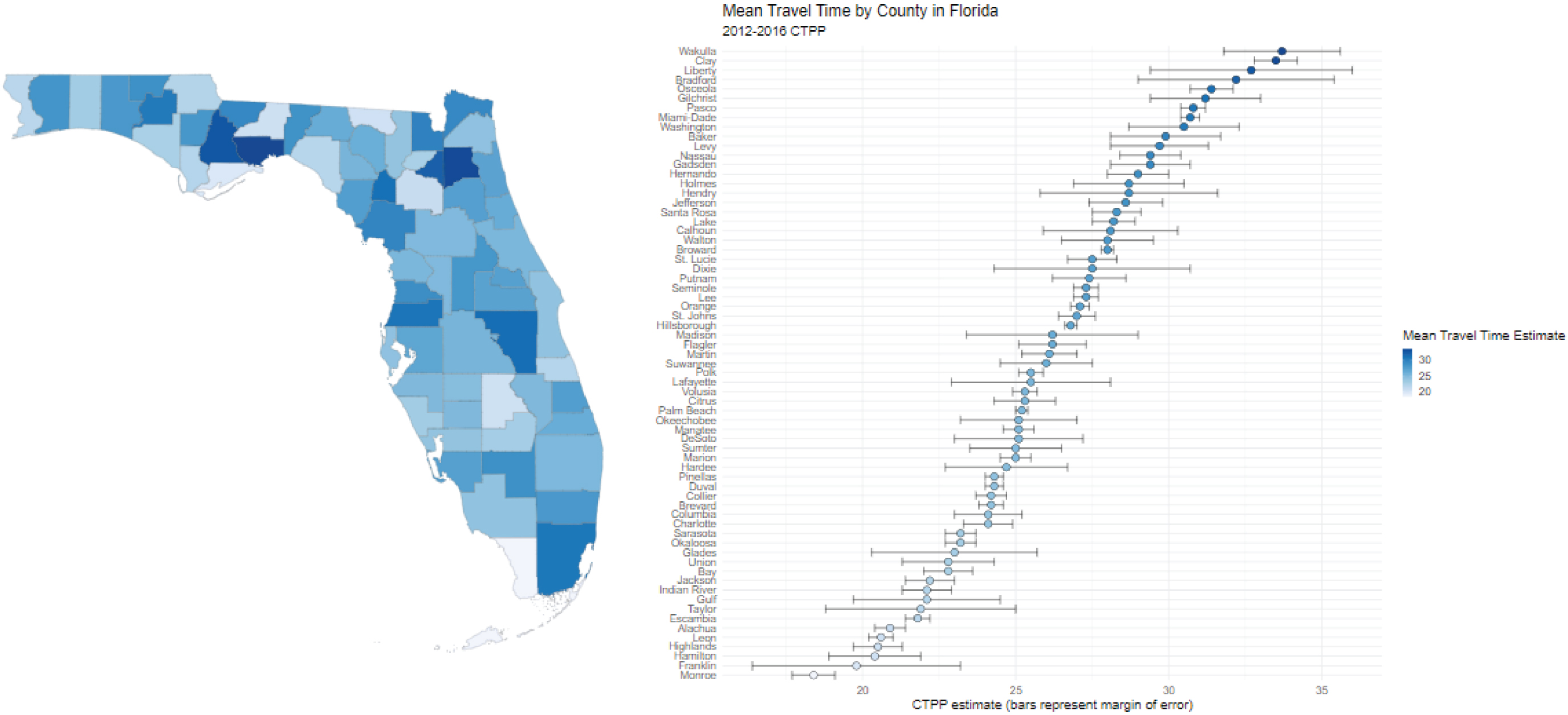
Long Description.
The map and a chart are placed side by side. On the left is a map of Florida with counties shaded based on mean travel time estimates from the 2012 to 2016 CTPP data. On the right is a horizontal dot and error bar chart showing mean travel time by county sorted from lowest to highest. Each dot represents the estimate, and the horizontal line represents the margin of error. Counties are listed vertically along the left axis, and the mean travel time is labeled along the bottom axis. The fill legend on the right shows the range of values used for shading both the map and the plot, with light shades indicating shorter travel times and darker shades indicating longer travel times.


