Constructing Valid Geospatial Tools for Environmental Justice (2024)
Chapter: 6 Indicator Integration
6
Indicator Integration
The White House Council on Environmental Quality (CEQ) Climate and Economic Justice Screening Tool (CEJST) technical documentation states that “disadvantaged communities face numerous challenges because they have been marginalized by society, overburdened by pollution, and underserved by infrastructure and other key services” (CEQ, 2022a, p. 7). This definition drove the committee’s discussion of disadvantaged communities (DACs) and the indicators selected to represent and measure this definition. This definition is also essential when considering CEJST’s approach to integrating the selected indicators into a single composite indicator and, ultimately, the designation of census tracts as part of a disadvantaged community. The process of integrating indicators into a composite indicator includes bringing all indicators onto a common scale, applying weights, and aggregating to a single value. Ideally, the process also includes evaluating the resulting composite indicator in terms of internal robustness, which has been shown to improve decision making and transparency in the integration processes (Freudenberg, 2003; Jacobs, Smith, and Goddard, 2004; Mazziotta and Pareto, 2017; Organisation for Economic Co-operation and Development [OECD] and Joint Research Centre [JRC], 2008; Saisana et al., 2019). Constructing a composite indicator is a widely used strategy for measuring cumulative burden and requires intentional decisions during each step of the process. Chapter 3 provided discussion on the construction of composite indicators. This chapter discusses those process components in the context of CEJST and their effect on the designation of census tracts as disadvantaged communities. The discussion also outlines alternative potential configurations that reflect cumulative impacts.
HOW CEJST INTEGRATES INDICATORS
As described in Chapter 5, CEJST comprises 30 indicators, each falling into one of eight categories of burden. CEJST converts most of the indicators into percentiles,
with a few exceptions that have natural cutoff values, including the presence or absence of abandoned mines, formerly used defense sites, and historic underinvestment in the form of redlining. The methodology then sets the threshold for each indicator at the 90th percentile. For indicators where a high value would be desirable (e.g., income or life expectancy), the values are inverted so that a high percentile value corresponds to a high disadvantage. In the sections below, the major decisions associated with indicator integration are discussed in detail.
BRINGING INDICATORS ONTO A COMMON SCALE
The goal of calculating a composite indicator is to combine different data types and measurements into a single measure or indicator to obtain as complete a picture of a complex, multidimensional phenomenon as possible (Mazziotta and Pareto, 2017). For CEJST, this means combining data on climate change, energy, health, housing, legacy pollution, transportation, water and wastewater, and workforce development. Within each burden category, multiple indicators are used, many of which use different measurement units. A measurement unit is the quantity used by convention to compare or express the quantified properties of specific types of natural, physical, or social phenomena.1 To meaningfully combine the indicators within these categories, they must have a common, scaled measurement unit to enable comparison or aggregation. Scaling refers to the process of transforming numbers such that they have a specific range of values (e.g., 0 to 100). The term “normalization” is used here as a general term for transforming numbers into common units with a common measurement scale for comparison or aggregation. Box 6.1 illustrates the process of normalization using the transportation category in CEJST as and example.
There is no one-size-fits-all rule about the best way to normalize indicators, but rather, there are trade-offs that need to be understood when choosing the most appropriate approach based on the concept being measured and the goal of the tool. There are several widely used normalization approaches in indicator construction, including min-max scaling, ranking, z-score standardization, distance from a reference, and categorical scales (often achieved using the calculation of percentiles). Mazziotta and Pareto (2017), the OECD and JRC (2008), Freudenberg (2003), and Jacobs, Smith, and Goddard (2004) explore these options and their trade-offs in a level of detail beyond the scope of this report.
The CEJST developers elected to employ a percentile approach to normalization and explained its rationale in its technical support document (CEQ, 2022a). The reasons provided include that percentiles (a) allow for identifying the relative burden that each census tract experiences compared to the entire United States and territories and (b) can be interpreted and easily understood by a broad range of users. Given the importance of building transparency, trust, and legitimacy as described in Chapter 3 framework for indicator construction, a normalization approach that is easily understood and inter-
___________________
1See National Institute of Standards and Technology, SI Units at https://www.nist.gov/pml/owm/metric-si/si-units. (accessed January 30, 2024).
BOX 6.1
Illustrating the Process of Normalization
The transportation category of CEJST includes three indicators with different measurement units: diesel particulate matter exposure, transportation barriers, and traffic proximity and volume. Diesel particulate matter exposure is measured in micrograms per cubic meter, while the transportation barriers indicator is calculated from the average relative cost and time spent on transportation relative to all other tracts. Traffic proximity and volume are measured as the number of vehicles on major roads within 500 meters divided by distance in meters. To combine these indicators into a composite, one might try adding or multiplying diesel particular matter exposure, measured in particulate matter per cubic meter (range of 0–1.92), with the traffic proximity and volume indicator, measured as the number of vehicles at major roads divided by distance in meters (range of 0–42,063.59). However, the large range of traffic proximity values would overpower the much lower range of particulate matter values, leading to an unintentional higher weighting of traffic proximity. While each indicator may be a valid measurement of a burden experienced by disadvantaged communities, they cannot be combined in any meaningful way until they have been brought into a common metric with consistent scaling because they are measured in different units and can have vastly different value ranges (Freudenberg, 2003; Mazziotta and Pareto, 2017).
preted can be valuable. The CEJST technical documentation (CEQ, 2022a) features substantial description and justification of how the percentile normalizing approach contributes to those end goals.
However, the CEJST technical documentation (CEQ, 2022a) does acknowledge the disadvantages of using percentiles for normalization. It can be ineffective for indicators that represent measurements that are poorly reflected on a linear scale, such as a bimodal distribution where there is a gap between the “good” and “bad” values of a given indicator. Percentiles can also mask or amplify the magnitude of difference between values. For example, CEJST uses the 90th percentile threshold on the indicator of low median income to determine if a census tract is designated as disadvantaged in the workforce development category. By this logic, a census tract at the 90th percentile is not considered any less disadvantaged than a census tract at the 99th percentile. By contrast, a census tract at the 89th percentile is not considered any more disadvantaged than one at the 0th percentile (i.e., the lowest level of burden). Using percentile normalization and thresholds for designating disadvantaged tracts has two important policy implications. Although the differential degree of burden experienced in tracts in the 89th and 90th percentiles may be slight, the resulting differential access to policy resources may be large. Moreover, the combination of data measurement uncertainties associated with input indicators (e.g., census margin of error) and the aforementioned propensity of
percentile normalization to mask differences in magnitude can diminish the capacity of percentiles to distinguish degrees of disadvantage.
Each normalization technique has strengths and weaknesses, and certain indicators and phenomena may benefit from choosing one approach over another. However, the resulting composite indicator is generally less affected by the choice of normalization algorithm than other decisions in the composite indicator construction process (Freudenberg, 2003; Tate, 2012). The lower influence does not mean that the normalization decision does not matter or that robustness testing around normalization techniques is not valuable. It does mean that if the decisions are considered and well documented, they are less likely to significantly influence the resulting composite indicator than other steps in the construction process.
WEIGHTING INDICATORS
As discussed in Chapter 3, once indicators have been chosen and normalized appropriately, the relative importance of each indicator with respect to other indicators in the final composite indicator needs to be determined. As described in Chapter 5, no explicit weighting is employed in CEJST to designate any single indicator as more influential than another on the resulting determination of a census tract as disadvantaged. No indicator is explicitly designated as more important than any other indicator. (Socioeconomic burden is implicitly more important because the socioeconomic threshold must be met in addition to any other indicator for a community to be designated as disadvantaged.) While explicit weighting is not employed in CEJST, it is important to discuss weighting and its impacts when integrating indicators using aggregation, given alternative aggregation approaches that might be applied by CEQ tools in the future. Decisions related to weighting indicators substantially affect the resulting composite indicator, both in terms of its actual values and its acceptance by technical experts and community members with lived expertise (Freudenberg, 2003; Saisana, Saltelli, and Tarantola, 2005).
Explicit Weighting
The calculation of a composite indicator can employ explicit weighting whereby individual indicators (or subindexes) are weighted during the aggregation process such that some indicators have a larger impact on the resulting composite indicator than others. Unequal weights are intended to reflect the differential importance of factors contributing to a composite measure (e.g., disadvantaged community [DAC] designation in the context of CEJST). The degree of relative importance can be derived from numerous sources, including policy objectives, scientific understanding, statistical methods, participatory approaches, and community preferences. Mathematically, weights are typically applied by simply multiplying an indicator before aggregating it with other weighted indicators, thus increasing or decreasing the relative influence of each indicator on the resulting composite measure. There is an art and a science to creating composite indicators and weighting. The methods applied are rarely clearly
right or wrong but rather a series of trade-offs and value judgments. The stated goal of the indicator and the definition of what is being measured can act as guiding principles when making these decisions, and the validity of the decisions can be tested through analysis and community engagement.
Many composite indicators do not have explicit weights assigned to each indicator (Freudenberg, 2003), and few of the environmental justice tools described in Chapter 4 use an explicit weighting scheme. Whether explicit (i.e., assigned coefficients) or implicit (hidden statistical structure), weighting is always present. Applying equal thresholds for each environmental indicator in CEJST is, in effect, a decision that each indicator equally contributes to disadvantage. Box 6.2 demonstrates how to explore the impacts of explicit weighting using CEJST downloadable data as an example.
Two common approaches for determining appropriate weights are participatory approaches and data-driven weighting approaches. Participatory approaches can be valuable when the goal of the indicator is to reflect the lived experiences of communities as accurately as possible (Mitra et al., 2013). It is important to the process to receive input from subject-matter and community experts on the impact of the chosen indicators on all their outcomes (discussed further in Chapter 7). There are also many data-driven weighting approaches based on the mathematical characteristics of the chosen indicators.
A common data-driven approach is factor analysis (FA) or principal components analysis (PCA) (Freudenberg, 2003; Mazziotta and Pareto, 2017; OECD and JRC, 2008). The OECD manual points out that while PCA and FA can be valuable for dealing with highly correlated indicators, they are not appropriate when the goal is to measure the theoretical importance of the indicators (OECD and JRC, 2008). The details of each of these methods are beyond the scope of this report but are described in Freudenberg (2003), Mazziotta and Pareto (2017), OECD and JRC (2008).
Each weighting approach has advantages and disadvantages, which require considering the trade-offs, particularly in the context of the purpose of creating the composite indicator and how it will be used. A challenge of explicit weighting is reaching a consensus among interested and affected parties and subject-matter and community experts about the weights used.
Implicit Weighting
Whereas explicit weighting represents a value judgment or policy choice about the relative importance of individual indicators, implicit weighting can occur due to the internal structure of the composite indicator. The magnitudes of intercorrelations and variances among indicators and the arrangement of indicators within the composite can affect the statistical importance of individual indicators. The result is a distortion of the relative importance imposed by explicit weights (Becker et al., 2017). Even when each indicator is assigned an explicit weight of 1, unintended implicit weighting may still occur within the composite indicator. Detecting implicit weighting is often conducted using Pearson correlation matrixes, which show the correlation coefficients between each pair of indicators. The idea is to use intercorrelations to evaluate the degree of
BOX 6.2
Exploring the Impact of Explicit Weighting
The “total categories exceeded” variable included when downloading CEJST “communities list data”a can be used to explore the effect of explicit weighting. This variable is the count of the number of burden categories where at least one indicator was exceeded for any given census tract. If a census tract meets the criteria for being designated as disadvantaged based on indicators in a single burden category, it would have a “total categories exceeded” value of 1. If a census tract met the criteria based on indicators in all categories, it would have a value of 8. Although not used to determine if a tract is designated as disadvantaged, this count variable can be used to visualize and understand the spatial distribution of the total categories exceeded variable. Figure 6.2.2 shows each census tract designated as disadvantaged, with darker colors representing tracts that are disadvantaged in more categories. This is currently the default rendering for the Justice40 dataset as shared as part of Esri’s Living Atlas,b a common place for the GIS community to access data and maps.
With no weighting, each category contributes to the resulting count equally, so the values range from 0 to 8, with each category adding either 0 or 1 to the count. If explicit weighting had been used, and, for example, the climate change category was weighted twice as high as the other categories, then the climate change category would contribute 2 to the resulting count instead of 1. Under these explicit weighting conditions, a census tract exceeding health and housing categories would have a count of 2 (and a tract that only exceeded the climate change category would also have a count of 2). The climate change category would have a larger influence on the resulting composite indicator than the other categories. Using this type of weighting can ensure that a composite indicator reflects the concept being measured, but it requires careful thought. Weights are multiplied by each indicator before aggregation when using an additive approach. When using a multiplicative approach, weights are used as an exponent for each indicator before aggregation, where each indicator is raised to the power of the weight (Mazziotta and Perota, 2017; OECD and JRC, 2008).
alignment between each indicator and the concept to be measured. The results can be used to filter out indicators exhibiting low statistical coherence. Indicators within the same dimension of the concept to be measured should ideally have moderately high positive correlations, while those with very high positive correlations signal potential redundancy (Sherrieb et al., 2010). Indicators with statistically insignificant or low correlations signify indicators that are potentially incoherent with the conceptual framework. An example correlation using a Pearson correlation matrix is provided as Box 6.3.
Correlation matrixes can also be helpful when evaluating the choices of indicators and an appropriate organizational structure. The current model structure of CEJST uses burden categories for thematic organization, but the categories serve no algorithmic purpose in determining DACs. If the aim of the burden categories is to ensure that

__________________
a See CEJST Downloads at https://screeningtool.geoplatform.gov/en/downloads (accessed January 30, 2024).
b Esri’s Living Atlas website: https://livingatlas.arcgis.com/en/home/ (accessed February 29, 2024).
the output composite indicator best reflects the concept being measured, alternative approaches to using nominal categories could be considered. This could include using true mathematical subindexes that have undergone statistical evaluation, as discussed above. The evaluation of an appropriate approach to categories includes considering if the structure of the composite indicator is coherent with the concept to be measured, both thematically and mathematically.
When indicators with correlation coefficients outside the desired range are present, there are several potential solutions. The first is to consider different or differently calculated indicators that better align with the conceptual framework (Sherrieb, Norris, and Galea, 2010). One recommended approach is to avoid aggregating negatively correlated indicators (Lindén, 2018). Techniques such as FA or PCA can be applied to statistically
BOX 6.3
Example Correlation Using a Pearson Correlation Matrix
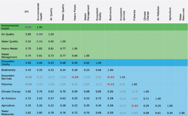
Figure 6.3.1 shows a Pearson correlation matrix of indicators in the 2020 Environmental Performance Index (EPI), which compares countries based on indicators organized into dimensions of climate mitigation, environmental health, and ecosystem vitality (Papadimitriou, Neves, and Saisana, 2020). Because they are within the same dimensions, the indicators assigned to the environmental health dimension (green background in Figure 6.3.1) should be positively and significantly correlated, and they are. The Joint Research Centre (JRC) audit of the 2022 EPI suggests an ideal range of correlation coefficients of 0.3 to 0.92 (Smallenbroek, Caperna, and Papadimitriou, 2023).a By this rule of thumb, the correlation coefficients for air quality (0.96) and water quality (0.96) in the environmental health dimension exceed 0.92 (green text in Figure 6.3.1) and are thus overweighted or potentially redundant. The presence of high implicit weights is often referred to as “double counting.” In the ecosystem vitality dimension (blue background in Figure 6.3.1), the correlation coefficients of several indicators are statistically insignificant (gray text) or negative (red text). Examples include the indicators of ecosystem services and fisheries. Because the correlations fall outside the ideal range, these two indicators are candidates for revision or removal due to low statistical alignment with the ecosystem vitality dimension. Because CEJST differs from the EPI in its constituent indicators, spatial scale, spatial heterogeneity, and organizational structure, different correlation thresholds may be better suited for evaluating implicit weighting and statistical coherence (Smallenbroek, Caperna, and Papadimitriou, 2023).
collapse multiple highly correlated indicators into a single multidimensional factor that avoids overweighting what they represent (Mazziotta and Pareto, 2017; OECD and JRC, 2008). Another option is to organize highly correlated indicators into subindexes, also referred to as dimensions, for the calculation of a composite indicator.
A subindex is a group of indicators within a composite indicator that have been combined to create an intermediate-level indicator. Subindexes are then combined to create the overall composite indicator (essentially forming composite indexes within the overall composite indicator). For example, if both diabetes and heart disease indicators are included in a composite indicator and are not combined into a subindex, this dimension of health would have a greater influence on the resulting composite indicator due to implicit weighting. Combining the two health indicators into a subindex would limit their outsized impact on the overall composite indicator. However, while using subindexes can address undesired implicit weighting, they can also be sensitive to the same challenges (e.g., if one subindex includes 2 indicators and another has 10, the values
__________________
a The Joint Research Center of the European Commission routinely conducts statistical audits of public policy indices. See https://commission.europa.eu/about-european-commission/departments-and-executive-agencies/joint-research-centre_en (accessed March 10, 2024).
of the individual indicators of the subindex with two indicators influence the resulting composite index more than the individual indicators in the subindex with 10 indicators).
The use of burden categories for thematic organization, but not mathematical subindexes, has implicit weighting implications. If the goal is for each burden category to have equal importance for the resulting designation of tracts, then the number of indicators within each category must be considered. Table 6.1 illustrates the share of indicators within each category of burden. Based on the methodology currently employed in CEJST, the categories of climate change, housing, and legacy pollution have 2.5 times the share of indicators used to designate a census tract as disadvantaged. This is not inherently right or wrong, but understanding the statistical impact of these decisions and justifying them is crucial to ensure that the resulting composite indicator is representative of the concept being measured. Mathematical subindexes would also benefit from a correlation analysis to help assess the alignment of the subindexes with the conceptual design of the composite index. If each subindex is intended to represent
TABLE 6.1 Number and Share of Indicators per Burden Category.
| Burden Category | Number of Indicators | Share of indicators |
|---|---|---|
| Climate change | 5 | 16.6% (5/30) |
| Energy | 2 | 6.6% (2/30) |
| Health | 4 | 13.3% (4/30) |
| Housing | 5 | 16.6% (5/30) |
| Legacy pollution | 5 | 16.6% (5/30) |
| Transportation | 3 | 10% (3/30) |
| Water and wastewater | 2 | 6.6% (2/30) |
| Workforce development | 4 | 13.3% (4/30) |
a different dimension of disadvantage, then highly correlated subindexes would require further investigation to ensure that they appropriately align with the intended design. For this reason, the conceptual framework outlined in Chapter 3 illustrates the importance of calculating a composite indicator as an iterative process, where decisions on integrating indicators, for instance, might lead to reevaluating the selected indicators and the organizational structure of those indicators.
The current CEJST technical documentation (CEQ, 2022a) does not mention any correlation analysis undertaken. Documenting any such analysis within the technical documentation would be valuable for interested and affected parties when evaluating the resulting DACs. If the analysis has not been done, performing and documenting the assessment would add rigor to the resulting designation of tracts and increase methodological transparency. The CEJST Technical Support Document (CEQ, 2022a, p. 7) states that “CEJST burdens are grouped into categories that were informed by Justice40 investment focus areas,” citing the White House Office of Management and Budget (OMB) Memorandum M-21-28 and Interim Implementation Guidance for the Justice40 Initiative (EOP, 2021), but does not offer further elaboration. The documentation also does not explicitly discuss the purpose of the burden categories, whether organizational or methodological.
Overall, indicator weights have significant impacts on the resulting composite indicator. If aggregation (discussed in the next section) will be performed, it is important to consider how each indicator will be weighted during the aggregation process. Explicit weights are essentially a value judgment, while implicit weights are data driven but can be poorly understood. Deriving explicit weights is complicated and sometimes contentious because they represent the relative importance of the different facets of the concept. As such, consensus on explicit weights can be difficult to achieve. Consequently, there is a tendency to apply equal weights to indicators and subindexes. Meanwhile, there is less frequent exploration of implicit weighting. This increases the possibility of producing a composite indicator with obscured statistical redundancy, input indicators with weak statistical alignment with the phenomenon of interest, and differential weights due to a varying number of indicators across categories. Correlation analysis can be applied to evaluate coherence with the concept to be measured, while
subindexes can be used to reduce bias introduced by uneven categories (Greco et al., 2019). With any weighting scheme, sensitivity analysis with the weights and visualization of individual indicators and subindexes can improve the understanding of the impacts of weights on model outputs and suggest remedies (Albo, Lanir, and Rafaeli, 2019; Becker et al., 2017; Dobbie and Dail, 2013; Räsänen et al., 2019).
INTEGRATION APPROACHES
Once the indicators have been normalized and weights have been chosen, the next step in constructing a composite indicator is to combine the weighted indicators into the output composite indicator. Two common integration approaches are threshold-based and aggregation approaches. As already described, CEJST employs a threshold-based approach based on a series of baselines that are used to decide if a census tract will be designated as disadvantaged. By contrast, an aggregation approach combines indicators mathematically, for example, by using additive or multiplicative approaches, to produce a continuous (i.e., noninteger) composite indicator. Aggregation approaches will be discussed in detail later in this chapter. Although the CEJST technical documentation (CEQ, 2022a) states that “disadvantaged communities face numerous challenges because they have been marginalized by society, overburdened by pollution, and underserved by infrastructure and other key services,” the implementation of CEJST stops short of reflecting those numerous challenges in their designation of census tracts as disadvantaged.
While each census tract has multiple opportunities to be considered disadvantaged based on the 30 individual input indicators (described in Chapter 5), the cumulative nature of burdens (or stressors) is not accounted for in a manner that is consistent with the description of disadvantaged communities above. Although each indicator is assessed based on both meeting the threshold for that indicator in addition to a socioeconomic burden, the cumulative nature of each category of burden (and even within a particular category of burden) plays no role in the determination of DACs. Further, the current designation logic obfuscates differences in the degree of cumulative impacts among the tracts designated as disadvantaged. This limits the capacity of CEJST to identify and prioritize the communities most in need. Redressing cumulative impacts is a policy objective of the White House (EOP, 2021), and the desire for CEJST to incorporate cumulative impact scoring is an objective of the CEQ and a common request of environmental justice advocates and analysts (CEQ, 2022a; WHEJAC, 2021). The closest that the current approach gets to cumulative impact scoring is by counting and recording the indicator criteria exceeded and the categories exceeded. As described in the discussion on weighting, these variables are provided as part of the data download, but they are not used in the final designation of tracts as disadvantaged.
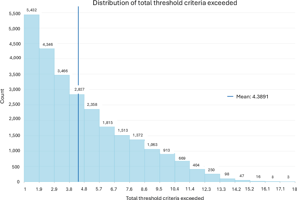
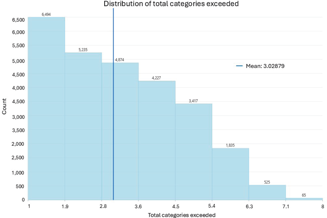
Figure 6.1 shows the frequency distribution of each measure in DACs based on data from CEJST, with the count of indicator criteria exceeded ranging from 1 to 18 (mean = 4.3) and burden category criteria exceeded ranging from 1 to 8 (mean = 3.0). The mode in each cumulative scoring scenario is one, comprising only 20 percent of the DACs based on thresholds exceeded and 24 percent of the DACs based on burden
categories exceeded. This means that within the collection of DACs, there are roughly three times as many DACs with multiple burden categories exceeded than with only one exceeded and four times as many tracts with multiple criteria thresholds than with only one. Hence, most DACs are subject to multiple forms of environmental disadvantage. This represents the proportion of census tracts that were designated as disadvantaged based on a single burden indicator or a single category of burdens. As described earlier in the weighting section, the count of categories can also be used to map and explore the number of categories that any given tract exceeded. Tracts that exceed the thresholds within more than one category are likely to experience more cumulative impacts than those that exceed one category. Employing such discrete scoring to model cumulative impacts would require no change to the existing CEJST computational structure but would result in a loss of information from percentile indicator values. It also amplifies the importance of the 90th percentile (burdens) and 65th percentile (income) thresholds.
An integration approach that uses aggregation is a common means to ensure that the presence of multiple stressors or the interaction between stressors is reflected in the resulting index. There are two commonly used aggregation approaches to reflect cumulative burden when calculating composite indicators: additive and multiplicative (OECD and JRC [2008] refer to these as linear and geometric, respectively). These aggregation approaches are more consistent with the research on cumulative burden and the emerging understanding of these issues, discussed in Chapter 2, accounting for the magnitude of stressors, the presence of multiple stressors, and the interactions across stressors. Additive aggregation methods commonly include sum and arithmetic mean, while multiplicative approaches commonly include a product and geometric mean. The technical details of these approaches are documented by Freudenberg (2003), Mazziotta and Pareto (2017), and OECD and JRC (2008) and are beyond the scope of this report. However, some important considerations of potential alternative approaches to be considered for CEJST are provided in the following section.
Existing EJ tools that incorporate cumulative scoring do so via an aggregation approach. For example, CalEnviroScreen2 employs a weighted sum of normalized indicators within two subindexes of pollution burden and population characteristics. The subindex scores are then multiplied to compute the index (CalEnviroScreen score), with tracts landing within the top quartile (25 percent) designated as disadvantaged. Maryland’s EJScreen Mapper3 adopts a similar mathematical approach. Its two pollution burden subindexes are averaged, as are its two subindexes of population characteristics. The resulting values are then multiplied to compute the index (EJScore). As opposed to the binary classification of indicator criteria or burden categories exceeded in CEJST, these aggregation approaches generate continuous values. If an aggregation methodology was used in CEJST, a threshold for DAC designation would be applied to the aggregation of conditions (like CalEnviroScreen) instead of to individual indicators.
___________________
2See “CalEnviroScreen 4.0.” California Office of Environmental Health Hazard Assessment, https://oehha.ca.gov/calenviroscreen/report/calenviroscreen-40 (accessed February 25, 2024).
3See “MDE’s Environmental Justice Screening Tool Beta 2.0.” Maryland Department of the Environment. https://mde.maryland.gov/Environmental_Justice/Pages/EJ-Screening-Tool.aspx (accessed February 25, 2024).
Such an aggregation scheme for scoring aligns more with cumulative impacts than the criteria-based one.
Considerations
When choosing an aggregation approach, a primary consideration is whether a high value in one indicator should offset or compensate for a low value in another indicator. This concept is known as compensability, and it drives many decisions related to aggregation (Mazziotta and Pareto, 2017). Compensability is defined by the OECD manual as “the possibility of offsetting a disadvantage on some indicators by a sufficiently large advantage on other indicators” (OECD and JRC, 2008). Additive approaches for aggregation are generally compensatory, while multiplicative approaches are generally partially noncompensatory.
Table 6.2 offers a hypothetical comparative example of how the aggregation approach affects the output index value. Community A has three indicators, all with a value of 2, and Community B has three indicators with values of 5, 0.5, and 0.5. With an additive approach such as a sum, Community A has a composite index value of 6, and so does Community B. With a multiplicative approach such as a product, Community A has an index value of 8, while Community B has an index value of 1.25. In the additive approach, despite Community B having two indicators with significantly lower values, the higher value for Indicator 3 compensates for the low values and leads to an index value in the middle. With the multiplicative approach, the two low indicators in Community B lower the overall index value substantially. This is because with a multiplicative approach, all values must be high to receive a high index value, and even a small number of indicators with low values will substantially decrease the resulting index.
A feature of noncompensatory approaches is that changes in indicators with low values will have a bigger impact on the resulting index than changes in indicators with a higher value. This means, for example, that a change in an indicator representing park access would have a bigger impact if park access were low. The same change in park access for a community that already has high park access would affect the resulting index less. Both characteristics of noncompensatory (often multiplicative) approaches need to be considered in the context of what is being measured and the goal of the index. In the context of cumulative burden, and specifically the ability of a composite indicator to reflect the presence of multiple stressors and the interaction between stressors, there are clear implications. If a high indicator value can be compensated for by a low
TABLE 6.2 A Hypothetical Aggregation Comparison
| Community | Indicator 1 | Indicator 2 | Indicator 3 | Additive Index Value | Multiplicative Index Value |
|---|---|---|---|---|---|
| A | 2 | 2 | 2 | 6 | 8 |
| B | 5 | 0.5 | 0.5 | 6 | 1.25 |
NOTE: Synthetic data are used for illustration purposes.
indicator value, and changes in low values are more impactful than changes in high values, then the ability to accurately reflect both the presence of multiple stressors and the interaction between stressors may be affected. Alternative approaches to integration that might be applied by CEQ in CEJST or some other tool in the future needs to involve considering the implications of compensability on the resulting composite indicator. For example, if an additive approach were used on the percentiles without an applied threshold, then very low values for a few indicators would dramatically change the resulting composite indicator and could compensate for one or two high indicators.
Table 6.3 explores applying an aggregation-based approach to the calculation for four real Justice40 census tracts where the percentiles for diabetes, asthma, heart disease, low life expectancy, and low income are all aggregated using both a sum (additive, compensatory) and a product (multiplicative, partially noncompensatory). The values for the health category for four distinct census tracts in the CEJST dataset are used to demonstrate the impact of the alternative approaches. The final composite indicator values are based on alternative aggregation approaches (sum and product) to the census tracts designated as disadvantaged based on the health category within the current CEJST implementation. In this example, the presence of a single percentile above the 90th percentile (the CEJST threshold) for any of the environmental indicators combined with a low-income percentile even close to the 65th percentile threshold results in a census tract being designated as disadvantaged, based on the current CEJST logic. The census tract in Florida exemplifies this strongly; the diabetes indicator is high, and the low-income percentile is high enough to meet the threshold, but the other three environmental indicators fall below the threshold. Using an aggregation scheme, the census tract is less likely to be designated as disadvantaged. Alternatively, the North Carolina census tract, with a similarly high percentile for diabetes and higher percentiles for all other indicators, is not designated as disadvantaged under CEJST logic because it just misses the low-income threshold (0.63 instead of 0.65). It would have scored as more disadvantaged than the Florida census tract using an aggregation scheme because of the accumulation of burdens across indicators. This accumulation is not considered in the criteria-based approach currently being used by CEJST.
The demonstration of compensability in Table 6.3 also illustrates the considerable influence that the low-income threshold has on the designation of census tracts as disadvantaged. For seven of the eight categories (i.e., all but workforce development), the current CEJST methodology requires meeting the low-income threshold for designation. A census tract could be above the environmental threshold for every single one of the 26 indicators within those seven categories and still not be designated as disadvantaged because of the simultaneous socioeconomic burden requirement. This is particularly concerning for places such as the North Carolina tract in Table 6.3, which is just below the 65th percentile threshold. In this manner, socioeconomic burden has a far greater influence on the designation of tracts than environmental burden.
TABLE 6.3 Effect of Aggregation Scheme on Burden Thresholds Exceeded
| Location (MPS code) | Category Indicator (CEJST percentile) | Sum | Product | Indicator Thresholds Exceeded in Health Category (max = 4) | ||||
|---|---|---|---|---|---|---|---|---|
| Diabetes | Asthma | Heart Disease | Low Life Expectancy | Low Income | ||||
| Louisiana, Orleans Parish (22071014000) | 0.99 | 0.97 | 0.99 | 0.93 | 0.99 | 4.87 | 0.88 | 4 (designated disadvantaged) |
| Alabama, Houston County (01069040700) | 0.87 | 0.83 | 0.87 | 0.84 | 0.62 | 4.03 | 0.33 | 0 |
| North Carolina, Forsyth County (37067001601) | 0.97 | 0.86 | 0.82 | 0.89 | 0.63 | 4.17 | 0.38 | 0 |
| Florida, Miami-Dade County (12086000410) | 0.96 | 0.85 | 0.76 | 0.34 | 0.68 | 3.59 | 0.14 | 1 (designated disadvantaged) |
NOTE: Darker boxes represent higher scores based on aggregation or thresholds. Federal Information Processing Standard (FIPS) code is represented in parentheses below the location in the first column.
SOURCE: Committee calculation based on CEJST 1.0 data.
Using Composite Indicators to Identify Disadvantaged Communities
A composite indicator calculated using an aggregation approach is almost always a continuous value. The example from Table 6.3 shows several calculations of continuous values for each census tract that could result from using an aggregation approach on the CEJST indicators. However, sometimes the goal of a composite indicator is to produce a binary categorization (e.g., a CEJST designation of disadvantaged or not). While the CEJST approach to integration is threshold based with a binary outcome, choosing to use an aggregation-based approach would not preclude a final post-processing step that allows for census tracts to be ultimately designated as disadvantaged.
For the aggregation sums and products of the four tracts in Table 6.3, a potential post-aggregation step could be a transformation of those sums or products to percentiles. Then, designation as disadvantaged could be based on the percentiles of those aggregated values. Similarly, a cutoff value could be applied to the final range of values based on subject-matter expertise, community input, or other methods. This would allow for an aggregation approach in the calculation of CEJST that results in both a continuous value representing cumulative burden and a designation of tracts as disadvantaged based on that continuous value. CalEnviroScreen is an environmental justice screening tool that uses this approach. After multiplicative aggregation, it designates tracts scoring in the top 25th percentile as disadvantaged.4
Any resulting composite indicator will be sensitive to choices made during normalization, weighting, aggregation, and post-processing, including the interactions between them. For example, careful consideration is necessary to understand the interaction between the aggregation approach chosen, the subindexes or categories of indicators being used, and the relationships between individual indicators. For this reason, a well-constructed composite indicator will need to be assessed using uncertainty and sensitivity analyses. Ideally, those analyses evaluate the impact of changes at each decision point to ensure that the goal of the composite indicator is being met. This type of assessment of robustness, along with thorough and transparent documentation of approach decisions and the impacts of those decisions, can also help build trust around the resulting composite indicator among users, decision makers, and community members.
ASSESSING ROBUSTNESS
Assessing the influence of uncertainty sources on policy benefits and costs provides valuable information to decision makers and the public (OMB, 2023). Model outputs are generally associated with two types of uncertainty: aleatory and epistemic (NRC, 1996). Aleatory uncertainty stems from intrinsic and unpredictable randomness in the phenomenon being modeled. Examples relevant to environmental justice (EJ) tools include ambient air pollution and disease incidence. Aleatory uncertainty is irreducible and is therefore represented in models using stochastic variables (Der Kiureghian and Ditlevsen, 2009). Epistemic uncertainty stems from incomplete knowledge of the
___________________
4See “SB 535 Disadvantaged Communities.” California Office of Environmental Health Hazard Assessment. https://oehha.ca.gov/calenviroscreen/sb535 (accessed February 27, 2024).
phenomenon being modeled. An example is imperfect understanding of the nature of interactions among environmental and social processes and the resulting influence on community disadvantage. Epistemic uncertainty can be reduced by integrating better data or improved knowledge into the modeling process. Quantifying and disaggregating uncertainty is the principal focus of robustness analysis for composite indicators.
As has been discussed, the construction of EJ tools, including CEJST, requires numerous modeling decisions for which plausible alternative choices are available. Ideally, such decisions are based on a detailed understanding of the concept to be measured. But with abstract constructs such as disadvantage that stymie direct measurement, composite indicator modelers must often make informed but subjective judgments. These judgments are a source of model-based or epistemic uncertainty; this arises when there is incomplete or imprecise understanding of how well factors such as the model structure, parameter values, spatial resolution, use of expert opinion, and data measurement represent the empirical processes the model is intended to reflect (Helton et al., 2010; Jakeman, Eldred, and Xiu, 2010). High epistemic uncertainty can lead to misalignment of real-world processes with the composite indicators that seek to represent them. Failure to consider and reduce epistemic uncertainty can result in negative policy outcomes and uninformed decision making (Maxim and van der Sluijs, 2011). However, it is often unclear which aspect(s) of a model construction process are the greatest uncertainty contributors.
Robustness analysis is a component of the committee’s conceptual framework for composite indicator construction (Figure 3.2) and can be conducted to meet multiple objectives. One objective is to assess the model’s statistical soundness or internal validity. Box 6.4 lists different types of analyses that are part of robustness analysis. Placed in the context of EJ tools such as CEJST, robustness assesses how certain the output designation of DAC status is for each census tract. Sensitivity analysis is the principal recommended methodology for assessing model robustness through quantifying overall model uncertainty and identifying the major source(s) of epistemic uncertainty (EPA, 2009). When subjected to sensitivity analysis, a robust model configuration will exhibit only a small change in the output in response to variations among the inputs. Another objective and important benefit of sensitivity analysis is that it can help differentiate the influence that input parameter options have on the composite indicator (e.g., those that greatly influence DAC designation and those that do not). Knowing this can enable the composite indicator designer to focus data collection and methodology development on the input factors that matter most, thereby improving the reliability of the model. Conducting sensitivity analysis on mathematical models is especially important when the model output is used in a policy framework in support of government regulations (Saltelli and Annoni, 2010). Boxes 5.3 and 5.6 in Chapter 5 provide two possible uses of sensitivity analyses in the context of indicator selection in CEJST, examining the PM2.5 and low-income variables respectively.
The first step in conducting a sensitivity analysis is determining which parameters will be evaluated (Greco et al., 2019; Munda et al., 2020). Table 6.4 displays examples of eight CEJST model parameters and associated options that could be subjected to sensitivity analysis. The items in boldface italics represent the options selected for the
BOX 6.4
Robustness Analysis Terms Related to Composite Indicator Development
Uncertainty and sensitivity analyses are the leading methods for assessing the robustness of a composite indicator. Robustness analysis is ideally integrated into the construction of a composite index for quality assurance. The following outlines the major aspects of composite indicator robustness analysis and their role in composite indicator construction.
Input parameter (alternatively called input factor in the sensitivity analysis literature) is a stage, step, or component of composite indicator construction. Within each input parameter, composite indicator developers must decide among plausible modeling options or choices.
Uncertainty analysis quantifies the overall variation in composite indicator output(s) based on varying input modeling decisions. Sources of composite indicator modeling uncertainty include parameter choices involving input data, arrangement of indicators into subindexes, imputation of missing values, normalization, weighting schemes, aggregation, and interactions among parameters.
Sensitivity analysis apportions variation in an output indicator to specific modeling decisions. It helps discern which decisions have substantial and minimal influence on the output.
Local sensitivity analysis evaluates the effect on the response of an output indicator to variations of a single input parameter. It is conducted by varying options within the focal parameter one at a time in calculating the composite indicator, while other parameters are held constant. The degree of local sensitivity is typically evaluated by examining statistical correlations or quantifying the percent change between realizations of the composite indicator.
Global sensitivity analysis evaluates the response of an output composite indicator to simultaneous variations among multiple modeling parameters. Uncertainty analysis is first done to determine the probabilistic distribution of the composite indicator, typically using Monte Carlo simulation. Variance-based sensitivity analysis is then applied to apportion the uncertainty to individual modeling parameters and uncover interactions among them.
construction of CEJST. This would be the baseline model configuration. The sensitivity analysis can determine which parameters have the greatest influence on determining whether a census tract is a DAC and which have the least. There are numerous methodological approaches for sensitivity analyses. The most common approaches are local (one at a time) and variance-based global sensitivity analysis (Saltelli et al., 2008). In local sensitivity analysis, the response of the output variable to variation of a single input parameter is evaluated by varying options within the parameter one at a time, while other parameters are held constant (Saltelli and Annoni, 2010; Xu and Gertner, 2008). The evaluation is straightforward to implement and often employs statistical correlation. If the resultant correlation coefficients are high, then one might conclude that the model is robust to variation in the parameter of interest.
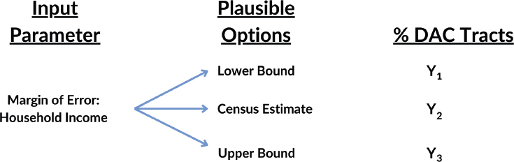
Figure 6.2 presents an example schematic of a local sensitivity analysis to assess the robustness of the margin-of-error parameter for CEJST’s income variable. Plausible discrete options within the error-margin parameter are evaluated while other parameters (e.g., indicator set, environmental burden threshold) are held constant. In this example, the output measure of interest is the percentage of disadvantaged tracts (Y). If the model is robust to changes in the margin of error, Y will change little across options. Correlation analysis or the percentage change in Y can be used to evaluate the alignment of Y across modeling options. The output variable Y could also be mapped to identify the tracts for which DAC designation remained constant and for which it varied. The analyst could then focus on the tracts with varying designations to examine if the model is performing as intended. See Jones and Andrey (2007) for a detailed example of local sensitivity analysis.
Local sensitivity tests are well suited for evaluating a single source of model uncertainty. However, they ignore and are unable to detect interactions among uncertainty sources that manifest not independently but jointly (Saltelli and d’Hombres, 2010; Tarantola et al., 2024). Local tests also become inefficient when the number of uncertain factors is large, but only a few are influential. In these instances, the ability to simultaneously vary multiple input parameters would be useful to interrogate the robustness of the current CEJST configuration, as well as potential future changes to CEJST, such as adding new variables or considering alternative percentile thresholds. Global uncertainty and sensitivity analysis are better suited to evaluate the sensitivity of a model to uncertainties in multiple input parameters.
In applying global sensitivity analysis to indicator construction, the objective is to quantify how variation in model output is apportioned to different sources of variation in the input assumptions (Saisana and Saltelli, 2008). This variation, or epistemic uncertainty, arises from subjective decisions in the selection among options for each input parameter. Uncertainty in these decisions propagates through the composite indicator construction to exert a combined impact on the output(s) (Saisana, Saltelli, and Tarantola, 2005). In global sensitivity analysis, options within multiple model construction phases are varied simultaneously via a two-stage process. First, uncertainty analysis is used to quantify the overall variation in model output based on varying modeling decisions. Sensitivity analysis is then applied to apportion the output variance to specific decisions (Razavi et al., 2021). Variance-based global sensitivity analysis is considered
TABLE 6.4 Potential Sources of CEJST Modeling Uncertainty
| Parameter | Example Options |
|---|---|
| Variable selection | Current 30 variables Alternative variable set Alternative variable set #2 |
| Measurement error on census variables | Ignore Sample within range |
| Imputation for missing data | None County average State average Regression Spatial interpolation |
| Normalization method | Percentile Min-max scaling Distance from a reference Z-score standardization Ranking |
| Environmental burden threshold | Value less than the 90th percentile 90th percentile Value greater than the 90th percentile |
| Socioeconomic burden threshold | Value less than the 65th percentile 65th percentile Value greater than the 65th percentile |
| Cumulative burden method | None Count of indicator criteria exceeded Count of burden categories exceeded Additive aggregation Multiplicative aggregation |
| Disadvantaged community designation | Count threshold =1 Count threshold greater than 1 Aggregation percentile threshold = 25 Aggregation percentile threshold = 30 Aggregation percentile threshold = 35 |
to be the gold standard for assessing the effects of uncertain model inputs on the variability of model outputs (Borgonovo et al., 2016; Saltelli et al., 2019).
In global uncertainty analysis, the model construction algorithm is subjected to a bootstrap analysis, in which the epistemic uncertainty associated with each decision parameter is propagated through the model. Monte Carlo simulation is employed to construct the model repeatedly, with each iteration generating the model output based on a random selection of the input parameter options. Instead of a discrete output value for each analysis unit (e.g., census tracts), the output of the Monte Carlo simulation is a probability distribution with a discrete mean, median, variance, range, and confidence interval. The Office of Management and Budget recommends reporting these statistics when conducting probabilistic uncertainty analysis for regulatory purposes (OMB, 2023). With use of the example in Figure 6.2, the probability distribution for CEJST
could determine the mean, range, and standard deviation of the percentage of census tracts designated as a DAC. Low values of the range and standard deviation would suggest a robust model, while high values would indicate model fragility. The mean value could then be compared with that of the CEJST configuration to assess if it is an outlier compared to the broader universe of potential configurations.
The results of the analysis could also be computed for individual analysis units. Potential descriptive statistics for the percentage of all census tracts designated as disadvantaged (percent DAC) output include the range, median, mean, and standard deviation. Figure 6.3 shows the results of a global uncertainty analysis from the JRC statistical audit of the 2022 EPI (Smallenbroek, Caperna, and Papadimitriou, 2023). The analysis evaluated the effect of varying methodological approaches for normalization, weighting, and aggregation on the output ranking of countries as the unit of analysis. The figure displays the median (blue dots) and 95th confidence interval (vertical lines) of the rankings of each country when all input modeling parameters are simultaneously varied in a Monte Carlo simulation. The countries are ordered from left to right in Figure 6.3 based on their ranking in the EPI. The confidence intervals show that the stability of the index rankings varies substantially across countries, with rankings robust for highly ranked countries but fragile in many other cases. To evaluate the robustness of the index, the audit’s authors deemed a country’s ranking unstable if the confidence interval exceeds 10 ranking positions, as is the case for 40 percent of the countries. This example demonstrates the utility of uncertainty analysis for both quantifying overall composite indicator fragility to alternative modeling decisions and identifying which analysis units have the most and least reliable ranks.
For CEJST, the large number of census tracts (>80,000) suggests mapping the uncertainty analysis outputs as opposed to charting them. This process of computation and geovisualization in uncertainty analysis would help discern the places with robust and fragile DAC designation. Consider the results of an uncertainty analysis in which overall variance is moderate, but high (low robustness) for disadvantaged communities. The results would help analysts zero in on which places have large uncertainty in the stability of DAC membership and further explore their environmental and demographic

characteristics. Within this smaller subset, other analysis options become available. A common approach is using a scatter plot (Greco et al., 2019), with the output (e.g., mean percent DAC) on the y axis and the uncertainty range on the x axis. Conversely, for tracts determined to be robust in the uncertainty analysis, there would be greater confidence in their DAC designation.
After epistemic uncertainty is assessed for the entire model or specific geographical areas, the next step is sensitivity analysis. Although uncertainty analysis can be used to estimate the overall degree of variability, it cannot determine which modeling decisions are the greatest contributors. Sensitivity analysis is thus applied to decompose the overall variance and assign proportions to individual input modeling parameters. In this fashion, the analyst could determine, hypothetically, that the choice of environmental burden threshold is responsible for 35 percent of the variation in percent DAC designation, while the normalization parameter is responsible for only 5 percent. In this scenario, the signal for future model development would be to focus on the burden threshold and not worry about the normalization approach. Sensitivity analysis can also be conducted to understand the impact that each individual indicator has on DAC des-
ignation using approaches such as a combined Monte Carlo–logistic regression (Merz, Small, and Fischbeck, 1992). Understanding which variables are responsible for DAC designation can provide quantitative insight into whether individual indicators are playing an outsized role in DAC designation. This can support an assessment of the choices of indicators and the formulation of the tool.
Ideally, uncertainty and sensitivity analyses are run in tandem (Saltelli et al., 2008). Unlike local sensitivity analysis, global sensitivity analysis can distinguish between main and interaction effects. An example of main effects would be the relative independent contribution of the socioeconomic threshold parameter to the total uncertainty (variance) in the output percentage of designated DACs. However, a portion of the total uncertainty may arise from interactions of the socioeconomic threshold with other input parameters. Such interactions can occur in composite indicators due to their nonlinear nature. For models with a low degree of interaction effects, understanding the influence of each input parameter is straightforward. However, for models with high interactivity, it is much more difficult. Table 6.5 provides a simplified decision-making framework based on the results of a global sensitivity analysis.
The examples in this subsection use the percent designated DACs as the output measure of interest. However, sensitivity analysis could also be applied to other output measures. These might include the number of indicators or burden categories that exceed environmental and socioeconomic thresholds, the demographic characteristics of DAC-designated tracts, such as total population, income, race, and ethnicity, and the geographic distribution of DAC tracts.
Assessing the impacts of epistemic uncertainties is a core best practice for quality assurance in indicator construction (OECD and JRC, 2008; Saisana et al., 2019) and is part of modeling guidelines adopted by the World Health Organization (WHO/ILO/UNEP, 2008) and the Intergovernmental Panel on Climate Change (Munda et al., 2020). Uncertainty and sensitivity analysis have been applied to prominent environmental and social equality composite indicators, including the EPI (Saisana and Saltelli, 2008; Papadimitriou, Neves, and Saisana, 2020), Human Development Index (Aguña and Kovacevic, 2010), Sustainable Development Goals Index (Papadimitriou, Neves, and Becker, 2019), and Commitment to Reducing Inequality Index (Caperna et al., 2022). Assessing epistemic uncertainty enables a deeper understanding of model structure compared to alternative assessment methods (Saltelli et al., 2008). Uncertainty and sensitivity analysis could help illuminate the implications of decisions made during model construction (WHO/ILO/UNEP, 2008; Tate, 2012). Applied to CEJST, the analyses could help guide future model development by revealing the
- Precision of model outputs,
- Dependency on fragile assumptions (corroboration),
- Modeling decisions that require the most additional consideration (prioritization),
- Modeling decisions that can be simplified,
- Combinations of modeling decisions that generate the most extreme values (exploration),
- Varying combined effects of modeling decisions (interactions),
TABLE 6.5 Sample Decision Framework Based on Global Sensitivity Analysis Findings
| Total Uncertainty | Main Effects | Interaction Effects | Model Uncertainties | Finding | Subsequent Modeling Focus |
|---|---|---|---|---|---|
| High | High | Low | Additive | Fragile | Reduce epistemic uncertainty for input parameters with high main effects. |
| High | Low | High | Interactive | Fragile | Reduce epistemic uncertainty for input parameters with high interaction effects. |
| Low | High | Low | Additive | Robust | Use the model as is or optionally reduce epistemic uncertainty for input parameters with high main effects to further increase robustness. |
| Low | Low | High | Interactive | Robust | Use the model as is or optionally reduce epistemic uncertainty for input parameters with high interactive effects to further increase robustness. |
- Places that would be designated under alternative modeling decisions (spatial distribution),
- Population characteristics of DACs under alternative modeling decisions (impacted populations), and
- Degree and location of geographic clustering of DACs shifts under alternative modeling decisions (spatial heterogeneity).
At present, these characteristics are not known, and uncertainty and sensitivity analyses have yet to be conducted, given the early stages of maturity of many national and state EJ tools. However, failure to consider and remedy uncertainty in modeling processes can result in poorly informed policy decisions. Given the high policy stakes of resource allocation tied to DAC designation, it is important to understand the effect of composite indicator modeling decisions on CEJST outputs. Box 6.5 provides an example workflow for uncertainty and sensitivity analysis that might be useful to CEQ.
Sensitivity analysis techniques are important tools for improving the robustness of models, increasing the transparency of the model construction, and ultimately increasing the validity of the model. However, uncertainty and sensitivity analyses only evaluate the internal statistical fragility of the model. It is possible to develop an analytically and statistically robust model that fails to faithfully represent real-world processes and conditions. As such, sensitivity analysis is ideally complemented by external validation against measurable quantitative or qualitative data. Validation is discussed in Chapter 7.
The approaches described in this chapter for data integration and robustness testing provide a strategy for CEQ based on tenets of composite indicator construction. However, the tool is not “complete” following integration and testing, even though the intended output has been generated. Performing analysis for other measures may help tools like CEJST—those with high degrees of complexity and policy implications—to become accepted by interested and affected parties and represent lived experiences. Performing external analysis demonstrates awareness of important issues associated with CEJST, adds transparency, and helps address concerns raised by affected parties throughout the model development process.
Two examples of external analysis with output measures are evaluating CEJST against race/ethnicity and geographic units. Although many interested and affected parties have advocated for the inclusion of an indicator of race into CEJST, CEQ stated that they do not intend to include race as a factor in determining disadvantaged community status (EOP, 2022). However, there are supplemental analyses that CEQ could produce to show the relationship between burdens and the racial composition of communities. Likewise, analysis of CEJST by geographic units (e.g., states, counties, or legislative districts) can lead to summaries of how disadvantaged communities are distributed throughout the nation, which is valuable for awareness and planning purposes. Supplemental analyses of measures external to CEJST are described in more detail in Chapter 7.
BOX 6.5
Potential Robustness Assessment Workflow for CEJST
Based on guidance for using uncertainty analysis and sensitivity analysis (UA/SA) in evaluating policy-relevant models from Munda and others (2020) and World Health Organization/International Labour Organization/United Nations Environment Programme (2008), the following is a potential workflow to incorporate robustness assessment into the data strategy for CEJST:
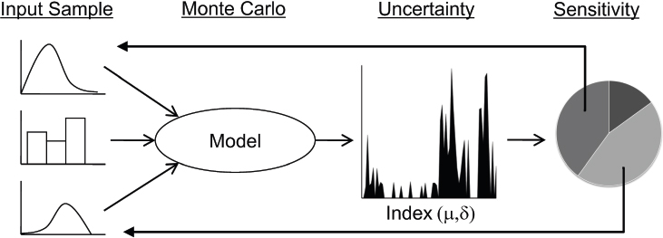
- An advisory group of UA/SA modelers, tool developers, community stakeholders, and scientific experts defines which input modeling choices to vary (treat as uncertain) and assigns a range or probability distribution to each to characterize the uncertainty. Figure 6.5.1 below portrays different probability distributions, while Table 6.4 provides examples of discrete distributions of plausible input modeling choices for CEJST.
- The advisory group defines the model output(s) of interest and the objectives of the sensitivity analysis.
- The UA/SA modelers randomly sample the previously defined probability distributions (Monte Carlo) to explore the entire uncertainty space. This corresponds to the Monte Carlo heading in Figure 6.5.1 below.
- The UA/SA modelers repeatedly run the model in a Monte Carlo simulation, using the values of the input samples. After each run, they record a value of the output(s) of interest.
- The UA/SA modelers quantify uncertainty measures based on the output distribution from the Monte Carlo simulation. The uncertainty heading in Figure 6.5.1 represents this.
CHAPTER HIGHLIGHTS
The process of integrating indicators in a composite indicator includes normalization, weighting, and aggregation. Normalization entails transforming input indicators into a common measurement scale to facilitate comparison. The primary normalization approaches include min-max scaling, z-score standardization, and percentiles. The CEJST documentation justifies the choice of percentile normalization, and research has shown that the modeling choice of the normalization approach has a negligible impact on a composite indicator.
Weighting is undertaken to inscribe the relative importance of each indicator into the composite indicator. Explicit weights are importance coefficients assigned to each indicator and are essentially value judgments based on scientific understanding, data-driven statistical analysis, participatory community preference, or policy priorities. Most composite indicators employ equal weights due to precedence or limited understanding of the relative importance of dimensions of the concept to be measured. The statistical properties and arrangement of indicators within a composite indicator can also produce
- The UA/SA modelers identify the most influential modeling choices and examine their potential impact on the CEJST model output(s) of interest. This is reflected by the sensitivity pie chart in Figure 6.5.1.
- The UA/SA modelers report the conclusions to the advisory group and prioritize areas for model improvement.
- Document the UA/SA process, including the data, methods, outputs, and interpretation of results, and communicate it using broadly accessible language. Include in the interpretation an assessment of the composite indicator’s precision, the credibility of the policy options, and the related policy impact.
obscured, implicit weights. Implicit weights can be revealed using correlation analysis, with the results used to revise indicators that are statistically redundant due to collinearity or have insignificant or negative correlations that indicate weak statistical coherence with the concept to be measured. Screening for implicit weights is an important element of composite indicator development, although the CEJST documentation provides no evidence that this was undertaken.
In indicator aggregation, scaled and weighted indicators are combined into a single measure. CEJST uses percentile threshold criteria on environmental and socioeconomic indicators to develop a binary measure of community disadvantage. This approach is simple and easy to understand, but the logic of indicator criteria exceeded is limited in its capacity to represent cumulative burden, which is a stated priority of CEQ and EJ advocates. Based on the existing CEJST structure, options for employing cumulative impact scoring include summing the count of indicator criteria exceeded or the count of burden categories exceeded. However, cumulative scoring through additive or multiplicative aggregation to a continuous composite indicator would better repre-
sent cumulative impacts, potentially reflect interactions among indicators, and discern disadvantage among communities.
Robustness assessment quantifies the statistical instability of a composite indicator when compared to alternative plausible modeling choices and identify which modeling choices have the greatest influence on that fragility. Uncertainty and sensitivity analyses are employed for these purposes and are a core practice recommended for developing policy-relevant models. The findings of a robustness assessment can iteratively be used to improve a composite indicator through revisions to the indicator set, normalization approach, weighting methodology, and aggregation scheme. CEQ could conduct uncertainty and sensitivity analysis on CEJST to quantify the influence of input composite indicator modeling decisions on the output designation of disadvantaged communities.


