Creating an Integrated System of Data and Statistics on Household Income, Consumption, and Wealth: Time to Build (2024)
Chapter: 5 Data Solutions, Methods, and Options
5
Data Solutions, Methods, and Options
While the three preceding chapters laid out the conceptual issues, the appropriate estimates and groups, and the problems associated with using existing data sources for producing income, consumption, and wealth (ICW) statistics, this chapter focuses on solutions. How can the goals and problems identified in the preceedings chapters be achieved? In addition, this chapter looks forward to the next chapter, because usability of the final product(s) is another important criterion for success.
Most of this report focuses on appropriate definitions and overarching goals for an integrated system of ICW data. While Chapter 4 identified an ideal data infrastructure, the current data infrastructure will likely not support producing this ideal dataset. The panel acknowledges that there will be tradeoffs between the various goals, especially between the data quality and concepts for ICW covered in the various data sources versus the ability of the public to access those data to produce their own statistics. In addition to choosing between input data sources, producing integrated statistics will involve “modeling” decisions, meaning methods for combining, imputing, or simulating one or more measures (e.g., wealth or consumption) given some observed measure from a base data source (e.g., income). The choice of data sources and methods bears heavily on many aspects of the integrated system of the ICW measures that is produced, including whether the system is a single file of comprehensive unit record data (“microdata”) or a set of summary statistics from joint distributions.
A variety of projects are underway, both in the federal agencies and by other researchers, each of which will provide new opportunities in
constructing an ICW integrated database. In a sense, all roads should be traveled. In this chapter the panel presents the alternative solutions for constructing an integrated system that includes ICW, drawing on current datasets of projects. The chapter provides the panel’s view of the best alternatives currently available to construct an ICW data infrastructure. This new ICW data infrastructure should be flexible enough to allow researchers to create their own measures for examining the important questions outlined in Chapter 1 and be consistent enough to enable federal agencies to create the statistics outlined in Chapter 3. While not focusing on one specific option, the panel believes that many options should be considered when investigating the best way to proceed in future.
STRATEGIES FOR MEASURING INCOME, CONSUMPTION, AND WEALTH
The panel’s starting point for laying out specific solutions is an overview of the potential strategies available for working with available data sources. A few broad strategies play a role in the data solutions discussed in this chapter. These include direct measurement of the population characteristics and ICW variables of interest, combining data sources using exact linkage, probabilistic linkage or statistical matching, using inference and imputation to solve for missing components, using alignment to match macro control totals, and achieving consistency between ICW using the intertemporal budget constraint.
Direct Measurement
Historically, the most pursued method for measuring population characteristics and components of ICW is direct measurement using household surveys. Surveys are generally designed to be representative of the population, and the surveys that collect components of ICW generally include the desired demographics as well. Household surveys are of course expensive to conduct, and low survey response rates (overall and item nonresponse) especially for some key ICW components are highly problematic and getting worse over time.
In recent years, direct measurement of ICW has increasingly relied on administrative data collected for some other purpose. Administrative data solves some of the problems with surveys but this introduces other problems. Response rates and reporting errors are less of a problem, because the administrative data are typically byproducts of some other government or private activity, such as tax collection, credit reporting, or public tracking of home sales. However, administrative records generally do not include the desired demographic information. Administrative data are also available
only for the relevant populations, meaning (in the examples) those who file income taxes, those who apply for and use credit, and homeowners.
Administrative data are also typically not designed to capture the ICW concepts the panel is trying to measure. Finally, some desired population characteristics and components of ICW are not available in any currently accessible government or private administrative data sources.
Incomes are generally the most available and conceptually consistent components of ICW available through administrative data sources, because of the federal income tax. Many of the important components of income (such as wages and salaries, interest, and dividends) are the same, conceptually, as the incomes subject to taxation. But other core income components in the conceptual ideal described in Chapter 4, including many types of government transfers and employer benefits, are not easily available because they are not subject to the income tax. Moreover, some income components, such as transfers between households, are not measured in any form in administrative data and are therefore available only in surveys.
Directly measuring household wealth for the purposes of building a large-scale annual ICW infrastructure is more challenging than measuring incomes. Much of the distributional analysis that has been done for household wealth is based on the Survey of Consumer Finances (SCF). This is mainly because of the novel method used to oversample high-income households. But, given its detailed questions about the composition of wealth (as well as income and population characteristics), the SCF struggles with high respondent burden and with nonresponse (like all government surveys) and is becoming increasingly difficult to conduct on even a triennial basis. There will be an important role in ICW statistics for a survey like the SCF going forward, especially in benchmarking imputations or linkages every three years. However, improving annual distributional estimates of household wealth will also likely involve capitalizing income data in the intervening years from tax returns (for financial assets that generate taxable income) and direct linkage, statistical matching, or imputation for other assets and liabilities, perhaps using private data on house values and outstanding credit.
Distributing household consumption is likely the most challenging within the overall ICW framework. The goal of the long-running Consumer Expenditure Survey (CE) is to collect detailed household expenditures (along with population characteristics and incomes) for a representative sample of the population. The CE suffers from extensive item and unit nonresponse, however, and there are no currently available government or private administrative data sources with extensive consumption detail. Some private administrative data sources (such as the JP Morgan Chase Institute) have made great strides in measuring selected components of
expenditure at the account level and could help fill gaps in direct consumption measurement (see Wheat, 2022).
Combining Data Sources
A key part of any ICW data solution is combining data sources, through either direct linkage or statistical matching. If one dataset (e.g., a Census survey or T13 Race and Ethnicity files;1 see Deaver, 2021) contains demographics for a representative sample of the population and the individuals in that sample can be linked to income tax or other administrative records, then problems with the survey-based ICW measures, such as item nonresponse and systematic under- or over-reporting, can be addressed.
To combine datasets, both exact and probabilistic linkages will be necessary. In blending some datasets, if Social Security Numbers (SSNs) are available on both datasets then exact matches are possible. Other datasets use name, address, and date of birth to probabilistically obtain an SSN for matching. Many of the federal files from the Social Security Administration (SSA), Internal Revenue Service (IRS), and Census Bureau have Protected Identification Keys (PIKs) already appended by the Census Bureau.2 This common person-level identifier will not solve all potential problems. If one of the data sources to be combined is not population representative—say it misses very-low- or very-high-income families—then the final product will need to be adjusted to correct for failure to systematically match certain types of records from the other data. These adjustments can include imputing or adjusting income, re-weighting the sample, or using additional sample. Moreover, between 10% and 40% of records, depending on the source, fail to have a PIK appended. Studies indicate that these records are not missing at random (see Brown, 2022; and Brown et al., 2023).
Identifiers such as PIKs (see Box 4-1 in Chapter 4) are becoming more widely available for linking surveys and administrative data (both U.S. government and private), and national statistical offices in other countries have made significant progress in this regard. Beyond person-level matching, there are important reasons to also link records of similar individuals—so-called “statistical matching”—as part of a broad ICW strategy. First, some datasets still lack PIK-consistent identifiers. Second, even if a dataset with complementary data could in principle be linked, access restrictions could prevent person-level matching.
___________________
1The Title 13 Race and Ethnicity File aggregates (and deconflicts) data from decennial census and household survey reports.
2PIKs are transformations of SSNs. People who cannot get a SSN (whether in the United States legally or illegally) may appear in administrative records and may have an Individual Taxpayer Identification Number but will not get a PIK (see Chapter 4, Box 4-2)
Statistical matching is an oft-used alternative method for combining data sources. The approach uses the common variables in two datasets (say population characteristics and income) to create joint distributions (say between income and consumption). Any systematic under-coverage or heterogeneity in the underlying datasets are of course problems for the combined dataset, and in addition, no inferences can be made about relationships between variables in the datasets beyond those associated with the matching variables. Until recently, computing power limitations restricted the ability to conduct the optimal statistical match (what is known as a constrained one-to-one match), but thanks to recent advances in the development of optimal transport algorithms, this kind of matching has now become possible. See Blanchet et al.’s (2022) “Real-Time Inequality” for an initial attempt.
Capitalization and Imputation
When directly measured ICW distributional data are unavailable or incomplete, the solution is to infer or impute values in an existing dataset using available information, and additional information from other sources. One key example of inference for financial assets is the technique of capitalization, which involves inferring wealth levels from the taxable income flows associated with a particular type of wealth (see Saez & Zucman, 2016; Zwick, 2022). Other types of imputations involve similar relationships between measured and unmeasured variables using auxiliary datasets.
Effectively implementing capitalization or other imputation strategies requires dealing with these sorts of heterogenous relationships using all available data resources, through record linkage and statistical matching. For example, estimates of financial wealth in a large-scale microdata file or a statistically collapsed (tabular) ICW dataset will generally involve capitalization. To maximize the accuracy of estimates one needs to mobilize all available evidence, including the SCF, to model potential heterogeneity in realized returns.
Alignment to Aggregates
The final component of the distributional tool kit is alignment, which takes two forms. First, in cases where available NIPA aggregates are conceptually consistent with a given ICW component, the distributional measures to obtain consistency between the aggregated micro and published macro value can be compared and possibly adjusted. Second, the intertemporal budget constraint that ties together components of ICW provides an important constraint on household- or group-level distributional statistics.
Consistency with macro control totals is often an objective when generating distributional ICW statistics, and simple forms of alignment such as scaling micro values to match the aggregate are often used as the tool to achieve that goal. However, like the other tools for producing distributional statistics discussed here, alignment should be implemented carefully. Many of the differences between micro and macro measures are due to the different definitions of resources such as income, or the lack of a specific variable in the micro-data that corresponds to the respective macro variable. However, in some cases, the lack of alignment is due to survey measurement errors or under-reporting. It is important to understand why micro and macro measures disagree.
Two alignment examples will help to show the complexities. The first is non-corporate business incomes (corresponding to income tax Schedules C, E, and F). The values reported to the IRS are low and declining relative to National Income and Product Account (NIPA) estimates. Indeed, the gap between IRS and NIPA is now roughly 50%—only half of NIPA noncorporate business income shows up on tax forms. Some of that gap is due to noncompliance, but some also reflects differences between taxable income as defined by the tax code and economic income as measured in the NIPA, most importantly the treatment of depreciation. Assuming tax data are used to produce income statistics for ICW, this could introduce a gap between the micro and the macro. Where in the income distribution does the missing NIPA business income belong? The Distributional National Accounts (DINA) literature attempts to provide guidance on this issue and present a variety of views and methods (see DINA guidelines [European Commission, 2024]; Saez & Zucman, 2020a; Zwijnenburg, 2019).3
The second example is consumption, whether in total or individual components. The aggregated available microdata (from the CE) are well below corresponding NIPA values, for all the reasons (population coverage, survey underreporting) mentioned above (see Bee et al., 2015; Passero et al., 2015; Sabelhaus et al., 2013). If the population were well represented and if everyone underreported spending in a consistent way, then applying a simple scalar would be appropriate. Certain categories of spending could be under-reported in the CE. Aguiar and Bils (2015) find that some categories are consumed differentially by the high-wealth families.
Consumption is also the primary focus of the second type of alignment in the distributional ICW data solutions toolkit. The intertemporal budget constraint discussed in Chapter 2 is an identity, assuming the ICW components are conceptually consistent. Indeed, the Financial Accounts of the United States (hereafter the Financial Accounts) publishes data series
___________________
3Section 3.1 pp. 26–29 on the specific issue of the gap between noncorporate business income in the NIPA and in the tax data.
showing the aggregate relationship between income, consumption, and change in wealth. The framework for those data series is the intertemporal budget constraint, and the divergence between NIPA saving and the Financial Accounts’ change in wealth (minus capital gains, which are not part of NIPA income and saving) is characterized as a statistical residual. With the new estimates for personal income and personal consumption expenditures at the Bureau of Economic Analysis (BEA)/Bureau of Labor Statistics (BLS), it would be useful to also include wealth from the Distributional Financial Accounts to fully examine the budget constraint at the macro level.
The same relationship between income, consumption, and wealth change holds at the household level and provides a potential check on other distributional statistics as well as a potential guide for adjusting those values. The caveat to using the intertemporal budget constraint as a guide is that it requires a measure of wealth change, not just the point-in-time wealth levels captured in datasets like the SCF. The implication is that using the intertemporal budget constraint to align ICW components at the household level requires income, consumption, and either (a) beginning and ending wealth or (b) direct measures of saving.
There is also an important downside to relying solely on the intertemporal budget constraint when constructing ICW micro files or distributional statistics. In many situations, it is important to know not only the total consumption, but also the components. The solution is to address consumption by using direct measurement with a dataset such as the CE, but—acknowledging the population coverage and reporting problems—use the intertemporal budget constraint to adjust components of consumption so the total is consistent with income and wealth (or saving). In addition, any measurement error present in a particular variable will also show up in the derived variable and thus induce a spurious correlation. For example, over-reporting of income given wealth will lead to overestimates of consumption (see Feiveson & Sabelhaus, 2019, for an example of using the budget identity to create the consumption measure).
Finally, building a longitudinal dataset with ICW is crucial to using the intertemporal budget constraint framework developed in Chapter 2, but it is also an integral part of the empirical strategy for meeting other objectives laid out earlier in the study. For example, much of what is important to understand about the size, direction, and impact of inter-household transfers, as well as the extent and causal factors that drive intra- and inter-generational mobility, can only be gleaned from longitudinal data (see Box 5-1 for more details on interhousehold transfers).
Another reason to develop longitudinal ICW datasets is the limitations of annual income and consumption along with point-in-time wealth snapshots. Such cross-sections are in many ways incomplete measures of economic wellbeing. Having multiple observations on annual income and
BOX 5-1
Measuring Transfers Across and Within Generations
As discussed, including interhousehold transfers is critical to accurately assessing the budget identity. However, measuring these transfers and how they impact wealth, income, and even consumption across generations requires data on both the transfers from donors and their effects on recipients. Most broadly, the preferred data are from a longitudinal panel that captures both the transfer donor and the recipient, the amount of the transfer (either cash or in-kind), and ultimately its effects on the recipient. Several cross-sectional and longitudinal datasets capture regular and irregular cash transfers from the donor perspective. But less is known about the recipients and the effect of the transfer on their longer-term economic position.a
More important for questions related to mobility over time or across generations are transfers that affect the household balance sheet. These transfers can be cash gifts paid or received or they can be debts paid or incurred. Consider, for example, what is needed in one key policy area—student debt—to understand how it affects younger generations as they emerge from college. In some surveys and in administrative data (e.g., IRS and Education Department), the accumulation of student debt is recorded, but not intergenerational support for college education. Such intergenerational support can take the form of either cash gifts across generations to pay college expenses or donations from a parent (or grandparent) who directly pays tuition and expenses, often from a college savings plan. To understand how such transfers or debts incurred affect the life chances of debtors and non-debtors, all of these elements are needed. At the recent meeting of the Organisation for Economic Co-operation and Development expert group on disparities in the NIPA, the importance of including interhousehold transfers in the measures of income distribution was discussed, including alternative data sources and allocation methods (see EG-DNA, 2023).
A longitudinal panel dataset should record all debts and assets and the sources of change in those net assets on an annual or biennial basis, across at least two (or three generations). Both transfers paid and transfers recorded need to be measured. The ability, or inability, to grow net wealth is antecedent to the ability to transfer wealth to others. Ideally, debts paid and transfers received, in cash or in kind, need to be measured over time for each generation.
Panel datasets such as the Panel Study of Income Dynamics (PSID), Health and Retirement Study, National Longitudinal Studies, Survey of Income and Program Participation (SIPP), and National Longitudinal Study of Adolescent to Adult Health all measure some of these transfers in cash on a regular basis. The advantages of an existing long-panel dataset are its ability to follow both donors and recipients across the life cycle, including transfers across at least two generations, and the fact that the
data are consistently measured over time and the protocols are already in place (e.g., consent). The disadvantages, however, are that each dataset measures a different cohort of the population and that expanding to the general population requires alternative methods (see also Chapter 4).
The Health and Retirement Study measures cash transfers made by donors and the receipt of transfers, for sample households. The PSID can measure transfers across two and three generations (see Pfeffer & Killewald, 2018). The Longitudinal Study of Adolescent to Adult Health records the event of a transfer, but not the amount of the transfer. The SIPP includes transfers to both parents and adult children (see Valle, 2023). Within generations, some types of debt are excluded (e.g., child support debt, prison related legal debt, medical debt) and some types of transfer are not recorded, including especially in-kind transfers (e.g., directly paying offspring’s college tuition; the sudden appearance of home ownership without affecting the new owners’ liquid financial position).
Although existing surveys lack comprehensive interhousehold transfers measured for both givers and receivers in a panel dataset, recent work with SCF cross-sections has shown it is possible to generate insights about the importance of transfers for understanding wealth dynamics. Obtaining the bequests given using a survey is difficult because that requires interviewing deceased individuals. However, one can estimate bequests using mortality rates and wealth levels, and researchers who have done so have found the estimated distribution of bequests to be well aligned with survey-reported inheritances received (see Feiveson & Sabelhaus, 2018). The SCF also asks questions about in vivos gifts made and received, and the CE asks about in vivos in-kind gifts made. In examining the SCF, the distribution of gifts made does not match the distribution of gifts received.
One obvious way is to build on existing survey instruments to broaden and deepen transfer data by including additional questions or more details about who the donors and recipients are. For instance, the 2021 SCF has added questions on legal debts and could also probe in-kind transfers across generations. In 2013 the PSID had a Rosters & Transfers Module that collected data on many of the constructs that are needed. This module could be refined, deepened, and included once again on the PSID or considered for other surveys (e.g., Health and Retirement Study or SCF). More research is needed to determine how best to use survey questions and administrative data to measure interhousehold transfers from both the donor’s and recipient’s perspectives and how to link the ICW integrated data system to longitudinal data that allow multigenerational comparisons.
__________________
a See the working group at the World Bank www.knomad.org/remittance-data-working-group. A complete accounting would also include remittances into the United States.
consumption for the same individuals makes it possible to study multiyear average “permanent” differentials in economic wellbeing as well as the volatility (and thus the risk of very low realizations) for income and consumption.
The discussion below does not provide details on how one might resolve the issues associated with moving from cross-sectional to longitudinal ICW data, largely because the options differ across the various ICW solutions. For example, pursuing the option to create a new panel with linked administrative data would present the opportunity to resolve issues of sampling and question wording that make existing longitudinal surveys problematic. If one constructs cross-sectional ICW datasets by starting with administrative records, the administrative records themselves will be the key to developing longitudinal files.
Indeed, longitudinal administrative frameworks are currently available, such as the work of Opportunity Insights (see Chetty et al., 2020; Friedman, 2022) linking tax and Census Bureau records longitudinally. In addition, there are internal projects such as the Census Bureau’s Decennial Census Digitization and Linkage Project (see Genadek & Alexander, 2019), and the Mobility, Opportunity, and Volatility Statistics (MOVS) project (see Jones et al., 2023). Another external project following similar processes to the MOVS project is the Income Distributions and Dynamics in America at the Minneapolis Federal Reserve Bank (see Kondo et al., 2023). The Intergenerational Poverty Panel (National Academies of Sciences, Engineering, and Medicine, 2023a, Chapter 11) recommends constructing longitudinal data to study intergenerational poverty using blended longitudinal data. Linking the ICW data to these datasets will only provide income longitudinally for the linked households, so obtaining consumption and wealth data would require imputation and modeling, as described in this chapter.
WHAT COULD BE ACCOMPLISHED WITH AVAILABLE DATA?
The analysis of data solutions begins with a question. What could be accomplished if the goal is to create a comprehensive ICW micro file using direct linkage between microdata files chosen to best capture the desired components of ICW? Such a dataset would aspire to meet the goals laid out in earlier chapters and employ the methods described in the first section of this chapter. Key features include comprehensive population coverage (including the top and bottom of the ICW distributions), demographic and geographic detail, and reconciliation with published aggregates.
The first step in developing a comprehensive micro file is to choose the base population data file. This defines what is labeled as the “spine” to which other microdata files will be linked. Ideally this would be a file with population-level coverage, likely starting with a population base or an
income tax base. The second step is ensuring that demographic characteristics and income (and tax) data can be accurately linked at the person level. The third step is to add wealth to the constructed population/income file; this will require a combination of direct linkage and modeling or imputation, because there are no linkable micro wealth data for many household wealth components. The final step is adding measures of expenditure and consumption to the population, income, and wealth file. As with wealth, some direct linkage is feasible in principle, but multiple goals for distributing consumption and expenditure suggest that some modeling or imputation will also be important.
Data solutions based on linking multiple administrative datasets and/or household surveys are increasingly prevalent. Chapter 4 reviewed international experiences with large-scale linked data files, which are becoming common in countries with comprehensive population registries. Examples of U.S. projects along these lines include the Administrative Income Statistics project and the National Economic Wellbeing (NEWS) project, both at the Census Bureau, as well as the Comprehensive Income Dataset (CID) produced by a University of Chicago team working at the Census Bureau (see Bee et al., 2023; Bee & Rothbaum, 2019; Medalia et al., 2019; Meyer, 2022; Rothbaum, 2022). These projects make great strides in the directions laid out in the previous chapters, but none is focused on a comprehensive view of the measurement of ICW, nor do they have comprehensive population coverage.
Population and Characteristics
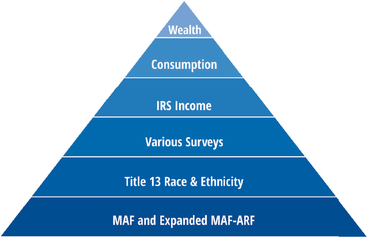
One starting point for building a microlevel ICW dataset is a population file with demographic characteristics—the so-called “spine” to which other microdata files will be linked. Starting with the Census Bureau’s Title 13 Race and Ethnicity File and Master Address File–Auxiliary Reference File (MAF-ARF), as used in projects such as NEWS and the CID, a population-based spine could support an integrated ICW data infrastructure. It could provide good population coverage and contain person-level and address-level linkage keys to facilitate joins to other microdata sources (see Figure 5-1A). In addition, these administrative data could be linked over time to form a longitudinal database (see Jones et al., 2023), which would be useful in creating longitudinal ICW data.
The main purpose of the ICW data is to obtain accurate annual data on ICW for households, including change in wealth (to obtain saving). As stated in Chapter 4, an ideal sample for the ICW data infrastructure includes all individuals in a household. Selecting a sample from a census population frame makes it possible to maintain flexibility in sample design. The new FRAMES project at the Census Bureau (Ratcliffe, 2021, p. 5) will
“[…] create Enterprise-wide frames linkable in nature, agile in structure, accessible for production or research on a need-to-know basis […]” The FRAMES project will enable linking the four frames at the Census Bureau (MAF, Business Register, Jobs frame, and Demographic frames). With appropriate permissions, a household survey sample (e.g., Current Population Survey Annual Social and Economic Supplement [CPS-ASEC], American Community Survey [ACS]) could form the base ICW cohort. Survey information on social, economic, and housing characteristics would be available, permitting analyses of individuals, families, and households based on survey-reported relationships. An ICW sample drawn from the population frame could also enable oversampling, as dictated by goals for geographic, racial/ethnic, and other decompositions.
One problem with the MAF is that it lists housing units and not people. The MAF-ARF includes the people who are included in a select set of federal administrative data (mostly tax data). Demographics and race can be obtained using the Title 13 Race and Ethnicity files. Linking a survey to that could add some people, for example those who do not file any tax returns or who were in federal administrative data with a Post Office box or rural route number instead of a street address.
Using the approach taken by NEWS is a good starting point, but there are potential improvements. The PIK identifiers used to link census datasets with other ICW files have also been used to create longitudinal files (e.g., the new MOVS project at the Census Bureau (Jones et al., 2023). However, the demographics in the spine file are generally only observed in the year the relevant survey is conducted. Some demographics are not available in the spine files, some people (e.g., homeless people and the extremely wealthy) are not included in the surveys, and some people are not linkable (see Box 4-1). Having access to a dataset that includes all individuals known to the U.S. government, complete with demographic characteristics, would substantially improve the spine (see Brown et al., 2023; Brown, 2022, panel presentation).4
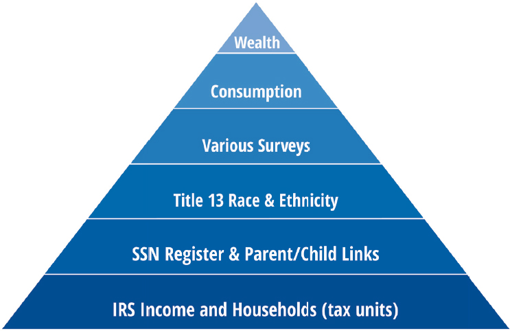
The Panel also heard about the possibility of using extracts of the tax data to create an income database (see Figure 5-1B; Larrimore et al., 2022). They suggest that these data could be used as a spine, with surveys and censuses providing the demographic content. This is similar to the approach taken by other countries, such as the Netherlands and Finland (see Chapter 4). As discussed by Larrimore et al. (2022) in their presentation
___________________
4There are coverage issues with using Social Security Administration (SSA) Numident + Decennial Censuses vs. Tax Panel. If you start with the Department of Treasury Administrative Tax Panel, you have stacked tax year datasets (information and individual income tax returns) with data the IRS has from its DM1 and DM2 (Numident and true Kidlink). Some people will be missing (e.g., people without SSNs, undocumented, unhoused, transient, students, seniors, group quarters, incarcerated). Adding additional data, as in the Census Bureau Administrative study (Brown et al., 2023) may improve coverage.
to the panel, the tax data can reproduce the coverage of households in the United States, although there may be some remaining issues concerning representativeness. As discussed in Chapter 3, it is important to be able to convert the tax data into income at the household level (see Box 5-2 for details on the coverage of the tax data).
These two core options consist of combining restricted data sources, which is most applicable for creating a restricted microdata file for analysts. These blended data include multiple data sources, with two different ways of determining the base or spine. Figures 5-1A and 5-1B demonstrate these differences. Figure 5-1A illustrates a method for using the MAF and MAF-ARF as the base to determine housing units (from the MAF) and individuals (from the MAR-ARF) by choosing the best person-place pair,
BOX 5-2
Who Is Included in the Tax Data?
The tax data can incorporate the 1040 along with the information returns; constructing useful data for household income is complicated by three issues. The main challenge with tax data is including the non-files. This information can be obtained from various other tax sources. The second issue is placing people into households using information on tax filers. The final issue is obtaining demographic information.
As presented by Larrimore (2022), people are excluded from the 1040 filings for a variety of reasons, such as being in noncompliance, having low incomes, having children who are not claimed as dependents, or being undocumented immigrants. Examining the third-party reporting such as data in 1099s or W-2s can yield more people. However, there are still some people who have no income with reporting requirements, such as those who have non-taxable sources or under-the-table income. With these techniques, the IRS population represented about 99% of the total decennial census in 2010.
In the tax data, there are about 35% to 40% more tax units than households. Creating households requires using the mailing addresses, which may be outdated or incomplete. Larrimore et al. (2021) use a variety of techniques to place people into households. For 2018, they find about 124 million households compared to the Current Population Survey (CPS) estimate of 129 million and the ACS estimate of 124 million.
Finally, the tax files only include age, sex, geographic location, and possibly marital status and number of children. Any race/ethnicity or other demographics are only obtained by imputation or linking to Census Bureau data or other datasets.
SOURCES: Based on panel presentation by Larrimore et al. (2021, 2022).
SOURCE: Panel generated.
and then using the Census Bureau’s special datasets for race (T13 Race from multiple Decennial Census Program data) and other demographics, and with survey data linked to this spine (see Brown et al., 2023) and IRS tax return and individual return data for income. Alternatively, Figure 5-1B illustrates a method for using the IRS data to determine the households and individuals linked to the Social Security demographic files, and similarly using the special Census Bureau databases (DM1 using the SSN register and DM2 for the Parent-child bridge files) to determine demographics (family relationships, age, gender, nativity, and place of birth). As with Figure 5-1A, a survey is then linked to this spine. For both methods, consumption and wealth are incorporated into the database using modeling, statistical matching, or linking with alternative commercial data. These diagrams could be expanded using Figures 4 and 5 in Bee et al. (2023) and presented by Rothbaum (2022). These figures illustrate the specific databases that can be linked by households and individuals.
Incomes, Taxes, and Transfers
ICW data should include person- and household-level income data with details on earnings, other compensation, capital incomes, taxes, benefits
SOURCE: Panel generated.
received, and transfers to construct the various broad income measures described in Chapter 2. When integrating individual income tax information, some income concepts are available at a person level and others at a tax unit level. Care must be taken to allocate income and tax burdens so that ICW measures can be made at individual, family, and household levels. Given linked incomes, any data solution will also have to address issues such as consistency between micro- and macrodata (as discussed earlier in this chapter). It will also need to address how to allocate incomes within households for person-level measures, and for longitudinal panel data it will need to link individuals over time as they change households and allocate income across households over time when households change composition, adding additional complexity (see Figures 5-1A and 5-1B for the different levels used for adding the tax data).
Other than IRS tax data, income data are available from federal and state agencies including the SSA, the National Directory of New Hires, and state labor market information offices (for quarterly wages used to administer Unemployment Insurance programs). Transfers are recorded by state and federal human services programs. These data are likely linkable to population-level files using personally identifiable information (e.g., SSN, name,
date of birth), and indeed many are already linked by the Census Bureau for their agency’s statistical purposes. The NEWS project already links some tax data provided by the IRS. So does the CID, which also integrates data that the Census Bureau has obtained from state human services programs, which include income and transfers received.5 These sources may include individuals with incomes below the tax filing threshold, an important group as is made clear in Larrimore et al. (2021), who noted that using information returns (e.g., 1099s) provides information on individuals not required to file an individual income tax return (1040). As discussed in Chapter 2, the tax data alone are not sufficient for generating total personal income, or many of the income definitions discussed (e.g., tax data do not contain information about the receipt of in-kind government transfers, imputed rent, or many interhousehold transfers).
Using the tax data and other administrative data linked to the survey data enables better estimates of the top and bottom of the income distribution. These linkages could be used to adjust the top of the income distribution in the surveys to better match the tax records. These methods have been utilized in the United Kingdom (see Jenkins, 2022). In the United States, BEA uses a simple adjustment factor for its distribution of personal income (see Fixler et al., 2020). Additionally, using both the tax data and the survey data may provide improved estimates of household income. In constructing the final estimates, alternative methods need to be considered, specifically those used in Bollinger et al. (2018), Han et al. (2022), or Bee et al. (2023).
Having comprehensive and detailed coverage across sources of income, taxes paid, and transfers is key for achieving the goals of improving the measurement of ICW. For example, it is important to know employer and employee pension contributions and the interest and dividends on retirement account balances for NIPA-equivalent personal income and disposable personal income measures, but also to know pension income received and withdrawals for the cash flow income measures used in distributional NIPA projects such as DINA and EG-DNA. However, some components are not readily available and need to be imputed (e.g., unrealized capital gains, health insurance benefits, and net imputed rent for homeowners; see below).
The panel’s goal of linking the best available data is to have incomes that add up to the corresponding NIPA totals. In situations where the linked microdata are the only administrative source data for NIPA statisticians, micro/macro consistency is generally automatic. There are,
___________________
5See Meyer (2022) for the importance of transfer programs such as Supplemental Nutrition Assistance Program, Temporary Assistance for Needy Families, and Women, Infants and Children in determining income.
however, situations where the linkable microdata do not add up to the corresponding macro aggregates, either because the NIPA rely on a broader array of raw data sources or because of conceptual differences (e.g., how income is defined). In all cases, assumptions must be made to distribute the portion of the macro aggregate that is not directly observable in the linked microdata.6 The envisioned linked micro file may well involve having multiple resolutions for the same discrepancies, each with different distributional implications.
Finally, a common theme for any proposed data solution is that incomes vary in terms of linking recipients at the individual, family, or household level. Wages are inherently an individual concept and can be aggregated by address. Transfer payments are often based on family eligibility, capital income accrues to just the owners of the underlying assets, and those sources can be disaggregated to individuals using different rules. As with decisions about reconciling micro and macro aggregates, flexibility in measuring economic wellbeing at the individual, family, and household levels should be part of any data solution.7
Household Balance Sheet Components
Household balance sheets can be divided into two main categories for the purpose of developing data solutions. Information about components of wealth not associated with direct income flows (e.g., owned housing, mortgages, consumer debt) is available every 3 years in the SCF and is often available annually via linking using a PIK-like identifier and access to proprietary administrative data. The components of wealth that are associated with capital income flows (e.g., business and financial assets) are generally unavailable in any single repository, but there are well-developed techniques for “capitalizing” the associated income flows for purposes of estimating asset values. It will be important to use both surveys and administrative data to validate the estimates. For example, the capitalization methods can be evaluated using the SCF and other microdata sources.
Microdata files with household balance sheet components for research purposes were largely nonexistent only a decade ago. New agreements and contracts between government, academic, and private organizations have given researchers access to individual credit bureau data (Equifax, Experian) and estimated values for some nonfinancial assets such as owned
___________________
6For example, to access proprietors’ income in both the NIPA and tax data requires examining how NIPA is constructed, what adjustments are made to the raw tax data, and what other input data are used. See Saez-Zucman (2020b).
7See Heathcote et al. (2023) on aggregating individual earnings to the household level.
housing (Black Knight, Zillow). In principle, a direct micro-link between the population/income file and these commercial sources would fill in those key components of the household balance sheet such as house prices, mortgage balances, and interest owed (for debt). In addition, the IRS has some data on accounts that receive tax preferences, and it may be possible to construct individual defined contribution account holdings or expected future pension benefits using a combination of individual information returns and plan-sponsor reporting. In her presentation to the panel, Quinby (2023) suggested that the IRS Form 5500 could be useful in estimating pension benefits.
What about private-sector data on wealth? There are still only a limited number of private-sector datasets on more comprehensive wealth. The two that have been explored are the Addepar (see Gabaix et al., 2022) and a dataset produced by Equifax IXI. These datasets are still very preliminary. Their advantage is that they represent data on actual wealth from wealth management companies and banks. Their disadvantage is that coverage is incomplete, not necessarily representative, and may not be at the individual level depending on data restrictions faced by the private companies. Data on ownership of real estate investments are potentially better; one could use deed records to measure real estate holdings, at least for owner-occupied housing. However, this may be difficult if people use trusts or a Limited Liability Company to buy houses. CoreLogic and other vendors currently have products that capture deeds for most of the United States.
Most of the remaining household balance sheet components are non-retirement business and financial assets, and those are not available through any single commercial database or other comprehensive data source. The approach to adding those components to the population/income microfile will thus involve some combination of modeling and calibration using available survey data.8 The panel heard about various projects using commercial data blended with survey data to estimate ICW. For example, Bucks (2022) discussed the use of credit bureau data and a survey to examine consumer debt, Friedman (2022) described the Opportunity Insights Affinity data to estimate income and spending responses, and Borzekowski (2022) presented the National Mortgage Database.
As discussed, capitalization is a possible approach to using reported capital inflows to impute wealth levels.9 Although there is a growing consensus that using a capitalization-of-income approach will yield a
___________________
8Another source of data on the value of durable assets may be from property insurance companies.
9The capitalization approach is at the heart of the sampling strategy for the SCF, because there are no microdata on wealth available for sampling purposes. It is thus not surprising that estimates of wealth inequality using the SCF are in close agreement with estimates based on the capitalization of high-quality capital income data.
distribution of financial wealth that is similar to that in the SCF, there are still limitations. For example, the relationship between capital income received and underlying asset values evolves over time because of changes in interest rates and how certain capital incomes are reported to the IRS. Understanding how interest received relative to asset values varies across individuals (for what appears to be the same sort of financial asset) is key to distributing the corresponding aggregate Financial Accounts totals for that asset type. In addition, the Financial Accounts aggregates required for capitalizing business and financial assets are themselves a statistical estimate, subject to error.
Capitalization requires making assumptions on how realized rates of return on assets vary with wealth within asset classes—for instance, how the rate of interest on interest-bearing assets varies across the wealth distribution. The simplest approach would assume that interest rates do not vary with wealth, though there is evidence that in some periods (e.g., 2008–2019) interest rates can rise with wealth. Researchers who have implemented the capitalization method attempt to take this into account, but this task is constrained by the lack of systematic evidence on the joint distribution of interest income and interest-bearing assets. Making assumptions is therefore necessary (see Fagereng et al., 2016; Saez & Zucman, 2016; Zwick, 2022). The accuracy of the assumptions and the sensitivity of the estimates to the assumptions have led to a vigorous debate in the literature that estimates the trends in top wealth shares using capitalization methods. Smith et al. (2023) and Fagereng et al. (2016) demonstrate that returns vary across wealth groups, and the timing of transactions can affect the reported returns, and they argue that the Saez and Zucman (2016) estimates may not be capturing this heterogeneity. The potential pitfalls associated with capitalizing income streams raise the issue of benchmarking the underlying methodology using the SCF or other high-quality microdata. The SCF suffers from limited sample size and frequency, but it is a key resource for studying the relationship between wealth and income. In addition, other emerging data sources (e.g., Bizcomps, DealStats) provide a more direct connection between business earnings and business valuations. Indeed, research using these and other data files (such as Zillow house valuations) has identified large gaps between aggregated micro and Financial Accounts wealth components, in some cases leading to changes in Financial Accounts methods for estimating household-sector aggregates.
Some combination of linking available micro wealth data and capitalization will cover all but a fraction of household balance sheet categories, and at a sufficient level of detail. Some additional wealth components, such as cars or fine art—each admittedly important for the bottom and top of the wealth distribution, respectively—are inherently connected to consumption and expenditure, as described in the next section. The asset value of
owned vehicles is also in many cases related to the vehicle debt that will be captured through links to credit bureau data. These sorts of micro-level consistency checks between ICW components are key for building a high-quality ICW microdata file. A current project, the Wealth and Mobility Study,10 is a joint statistical research project between the IRS and the Stone Center for Inequality Dynamics that will create a database of wealth using the IRS data to provide wealth and income information across time by detailed geographic areas.
Consumption and Expenditure
Adding consumption and/or expenditure to the envisioned ICW microfile comes with many of the same challenges as adding income and wealth. Moreover, two important additional considerations must be taken. First, consumption is a direct measure of economic wellbeing. Second, spending is the key to understanding saving and wealth accumulation. These two goals necessitate flexibility in consumption and expenditure categories, because some components (e.g., food) are in both, whereas others (e.g., health care, interest and principal paid on a car loan) show up differently in consumption and expenditure, and those differences are in turn associated with what the panel means by income and wealth. In addition to categorical flexibility, having the two goals in mind is also important for choosing between methods for filling in those categories.
As is the case for incomes and some wealth components, for spending there are potentially linkable administrative data from private-sector sources. For example, researchers at the JP Morgan Chase Institute have used customer transactions data to estimate spending (as well as many forms of income). In principle, customer spending records could be linked to the ICW, to the degree that the samples overlap, and thus provide direct, high-quality information on the components of spending captured in those transaction data. Other researchers have used “financial aggregator” approaches to capturing transactions recorded by financial institutions. One shortcoming to using transactions data is coverage, because some transactions use payment methods outside the scope of what is captured by the financial institution(s) whose data would be linked. For example, administrative records from credit card companies will not capture most vehicle purchases, because credit cards are not typically used to purchase cars.
The main expenditure survey in the United States is the CE, sponsored by BLS and collected under contract by the Census Bureau. In principle, one could link its survey responses to the ICW file (see Hong et al., 2023 and Brummet et al., 2018, for linkages between the tax data and CE data).
___________________
The CE aspires to derive a comprehensive measure of consumer spending, thereby overcoming the coverage problem with transactions data. There are well-known discrepancies between CE and NIPA spending data, however, attributable to both population coverage (very wealthy households generally do not participate in the survey) and the methodology itself. Research suggests that high-income households may under-report their high level of spending (see Aguiar & Bils, 2015; Sabelhaus et al., 2013). Linking the CE to the population/income spine would help in identifying nonparticipants and whether they are likely high-income (see Bee et al., 2015; Sabelhaus et al., 2013), and also help in identifying CE respondents who are in the spine and may under-report their incomes.
The approach of linking either person-level transactions or CE data to the sample chosen from the population/income spine draws attention to the question of discrepancies between measured ICW (see Brummet et al., 2018; Hong et al., 2023). Again, as with wealth and income, some combination of linking and modeling will lead to the best distributional estimates. The proposed strategy is to account for inconsistencies using two approaches: direct and indirect. This could be done either by linking as much spending as possible from transactions data or the CE to measure consumption or by using the four-quarter longitudinal nature of the CE or the 2-year changes in the ICW file to measure total spending as the residual implied by the intertemporal budget constraint.11 Total spending is the difference between the change in wealth and disposable income. The competing approaches will generally disagree about total spending, but (a) each category in the NIPA has only one aggregate value, and (b) the best possible answer will come from simultaneously addressing what can go wrong with either direct spending estimates or the spending implied by the intertemporal budget constraint.
Tying this back to underlying research questions, resolving discrepancies between directly measured spending components and implied total spending based on income and wealth from both directions is key because one wants to preserve the information about both spending components and saving. Separating spending on food, housing, education, transportation, and health is important for an analysis of economic wellbeing at the bottom of the ICW distribution. Validating total spending measures using the intertemporal budget constraint is key for studying saving and wealth accumulation at both business-cycle and life-cycle frequencies. Both are important goals and warrant the effort that will be required to distribute spending across households in a way that respects what is known from aggregate totals, transaction or survey spending, incomes, and wealth.
___________________
11Modernizing the consumer price index report (National Academies, 2022) recommended using commercial data to improve the CE expenditures.
Finally, even after resolving spending by category, the issue of consumption vs. expenditure is still relevant. Some consumption is in-kind, such as government-provided or subsidized health care or housing. Some consumption is a service flow associated with owned vehicles or housing. As with the discussion of income above, the goal is to create a dataset with sufficiently detailed variables that will allow researchers to create alternative measures of total consumption or spending that pull together the various pieces. For example, one can and should measure outlays for new vehicles, which correspond to the new car “consumption” in NIPA, but also keep track of the loan balance and flows of interest and principal payments that make it possible to construct a service flow measure. In many cases, such as government health care, there are decisions about whether to allocate the insurance value or actual health care outlays for a given individual, as well as how the individual should value those benefits. The choice will likely vary by researcher, and the implication from a data-solutions perspective is to ensure that the associated income is consistent with the definition of consumption. For example, including in-kind benefits in income requires also including them in consumption.
Another method to improve spending estimates is to incorporate commercial data on transactions. Wheat (2022), Hansen (2022), and Shapiro (2022) presented to the panel options for using credit card transactions (i.e., the JP Morgan Chase Institute data) or retail firm transactions (via Nielsen scanner data, see Ehrlich et al., 2023) to create measures of household spending (see also Buda et al., 2022). In fact, the Modernizing the Consumer Price Index for the 21st Century report (National Academies, 2022, p. 15) recommends that BLS “[…] invest in collecting comprehensive data for individual spending using electronic means of payments such as credit/debit cards or other electronic payment processors (e.g., PayPal or Stripe).” Currently, both BEA and the Federal Reserve are creating weekly spending measures using First Data card transactions (see Batch et al., 2023). It might be possible to link these commercial data, even at an aggregated level such as by ZIP Code, to the CE Survey data and the ICW data infrastructure.
Building this blended data on ICW requires coordination across agencies to link the data and provide access to the data (see National Academies, 2023a). The panel suggests that the alternative models (in Figures 5-1A and 5-1B) be constructed with the guidance of the Office of the Chief Statistician to create a coordinating entity that will help create the infrastructure in the next 1 to 3 years (see Box 5-3 for details on the coordinating entity).
BOX 5-3
Creating a Coordinating Entity
As discussed in Chapter 1, the Chief Statistician works with the Interagency Council on Statistical Policy to coordinate projects across statistical agencies, with a new supporting entity of the National Secure Data Service (NSDS). The NSDS will hopefully serve as a hub for data integration activities across the federal government and includes a pilot project with America’s Data Hub. Given that different agencies have various levels of access to surveys, administrative data, and linkages, it is critical that the coordinating entity for the ICW project housed outside of the relevant statistical agencies. While the details of what this will look like are not yet clear, the NSDS would be a natural choice for coordinating the creation of the data products envisioned by the panel. Possible roles for the coordinating entity include:
- Working with stakeholders, agencies, and researchers to develop methods and estimates to be released (as in Recommendations 5-2, 5-3 and 5-7).
- Working with agencies and nongovernment sources on data acquisition, integration, exchange, access, and possible collection (as in Recommendations 5-6 and 5-7).
- Managing linkage and production efforts to generate files and statistics on a schedule, and work with Phase 2 to manage researcher access (as is described in Recommendation 6-5).
- Handling financing (from both agencies and nongovernment sources) of data acquisition, collection, and linkage.
- Collaborating with relevant statistical agencies to assess options for researcher access to ICW microdata through an NSDS (as stated in Recommendation 6-1).
- Collaborating with the steering committee (Recommendation 6-3).
- Encouraging and coordinating inter-agency pilot projects (see Recommendation 5-2 and roadmap in Chapter 6).
RECOMMENDATION 5-1: The Chief Statistician and the National Secure Data Service should work together to create a coordinating entity to solve administrative, legal, and technical challenges to integrate data from multiple federal entities (e.g., Bureau of Economic Analysis, Census Bureau, Bureau of Labor Statistics, Statistics of Income) as well as private businesses that collect microdata on individual and household income, consumption, and wealth. In the near term, the coordinating entity will codify agreements and protocols that enable data acquisition, integration, exchange, and access, and support the publication of privacy-protected statistics.
The ICW data infrastructure relies on the various internal projects already underway in the federal agencies. Each of these projects, coupled with the ideas presented in this chapter, will provide a useful framework for building the ICW data and producing the ICW statistics described in Chapter 3. However, helping the agencies collaborate and improve their data and estimates requires the coordinating entity to expand on current efforts and incorporate best practices across the agencies. One method of moving the process forward is to organize pilot studies. For example, expanding NEWS to include government in-kind transfer programs, health benefits, income taxes, and capital gains, or building on efforts to measure spending in commercial data to improve consumer expenditure data in the CE, or evaluating both data constructions shown in Figures 5-1A and 5-1B to compare the estimates of income and population characteristics, particularly in the tails of the distributions. In addition, related to the budget identity, a comparison could be undertaken of the consumption (or spending) estimates using the budget identity or actual estimates (e.g., see Feiveson & Sabelhaus, 2018; Fisher et al., 2022).
RECOMMENDATION 5-2: In the near term, the coordinating entity working with the relevant agencies should expand on current efforts and coordinate new pilot studies to blend multiple datasets that have the key components of income, consumption, and wealth; develop and refine modeling methods appropriate for household income, consumption, and wealth (including an income capitalization option); perform statistical matching to combine information from multiple data sources; fill missing population groups using synthetic records; and impute missing information using relationships estimated in ancillary datasets.
RECOMMENDATION 5-3: In the near term, the coordinating entity should work with the relevant statistical agencies to ensure that they publish comparisons of linked income, consumption, and wealth (ICW) data relative to the conceptual framework and budget identity relationships between ICW, in conjunction with their release of ICW data and estimates. Doing so will gauge the internal consistency between ICW/wealth change at the micro level.
WHAT COULD BE ACCOMPLISHED USING PUBLICLY AVAILABLE DATA?
While the previous section examined creating an ICW dataset given unfettered access to all existing government and private data sources, this section examines the question from the opposite starting point: What could
be accomplished if the coordinating entity were restricted to use information that is already in the public domain? A public-domain-based ICW would presumably be less costly and quicker to create, and it could be released to the public without concerns about confidentiality. It could also serve as a “bridge” project for a coordinating entity as it awaits funding and navigates legal hurdles associated with creating an ICW dataset based on more comprehensive and more sensitive information. The advantage of working to build ICW using public data is that research can start soon and does not require obtaining special access. But as will be evident, the value of the end-product would be much more limited.
Tables 4-1 through 4-4 in the previous chapter reviewed the publicly available and freely downloadable microlevel data sources on income, consumption, and wealth that might be combined to create a public-domain-based ICW dataset. Information about various types of income is available in the CPS-ASEC, ACS, SIPP, SCF, CE, and IRS public-use samples. Information related to consumption is available in the CE, and information about wealth is available in the SIPP, and the SCF contains some components of consumption (see Fisher et al., 2022). As shown in Tables 4-1 through 4-4, the CE provides the only dataset with measures of ICW (see Garner & Short, 2013), although wealth is missing for a large share of households. Chapter 4 also reviewed the shortcomings of the different microdata sets, including (depending on the dataset): incomplete population coverage, low frequency, small sample sizes, limited demographic information, and underreporting of some types of information.
Table 4-2 of the previous chapter lists ongoing projects that aim to overcome the limitations of individual data sources by combining various U.S. microdata sets. Among these projects, Fisher et al. (2022) stand out as the only one that does not require access to restricted sources. Their study focuses on examining the joint distribution of ICW using the SCF as the foundational dataset. To improve on the SCF income measure, they incorporate capital gains and use the National Bureau of Economic Research (NBER) TAXSIM model to estimate taxes. They also impute a more comprehensive consumption measure using information from the CE as well as a limited set of consumption items from the SCF. This project serves as a good example of how to create a public-domain-based ICW dataset, especially one with a fairly narrow objective that requires the accurate measurement of the wealth of the highest-income households. However, this dataset has limitations that might be obstacles for other research questions. For instance, the SCF is conducted only every 3 years, lacks information on pension wealth (although Jacobs et al., 2021, demonstrates how pension wealth can be estimated using synthetic-cohort methods), lacks important
background information about households (such as geography), and has a sample size that is too small to address significant wealth-related questions (such as many aspects of the racial wealth gap).
A broader approach would be to build off a larger dataset that has some information about income, consumption, and/or wealth as well as comprehensive data about demographic traits, family characteristics, and geography. The CPS and the ACS would be suitable to serve as the base data for this purpose (the spine discussed above is broader than just a household survey). The first step would be to evaluate the population coverage—the CPS, for example, has been documented as lacking coverage of the very top and very bottom of the income and wealth distributions. The next decision would be whether to improve effective coverage by modifying the records close to those that are missing or incomplete or by adding additional synthetic records.12 Of course, as with all choices made in creating a public-domain-based ICW database, the costs of simply living with limitations such as incomplete population coverage would need to be weighed against the potential for leading researchers astray with imperfect estimates. The latter part of the calculation could be informed with exercises that “check” the estimates against information from independent sources known to have some degree of accuracy (see Chapter 4 for possible quality measures and the importance of linkage errors).
A key challenge for creating a public-domain-based ICW database is that, in contrast to the approach described in the previous section, the publicly available microdata files cannot be linked directly because of the lack of PIK-like identifiers (and even if such information were available, the overlap of the different datasets might be insufficient to create a large representative sample). Therefore, combining data sources requires statistical matching—linking similar observations across sources based on common variables. For example, better information about income in the CPS-ASEC might be attained by assigning values for missing income components (or those known to be poorly measured) based on information about similar households from the administrative records in the IRS public-use files. Similarly, key components of wealth might be estimated for CPS-ASEC records using statistical matching with the SCF, as well as matching with the IRS public-use files for wealth components that are better captured by capitalized financial income. Finally, consumption might be added to the CPS-ASEC through a statistical match with the CE.
As researchers have long recognized, the results of statistical matching may suffer from a variety of problems. Relative to actually linking datasets
___________________
12See www.sciencedirect.com/science/article/abs/pii/S0921800922003597 and https://arxiv.org/pdf/2006.01686.pdf
with different information about the same individuals, there will be a general loss of precision in the information that is estimated using matching. The measurement error may also be correlated across individuals if there are systematic differences in characteristics not used for matching. For example, the SCF lacks information about geography, and the resulting inability to match on this information would likely lead to overestimates of wealth for CPS households living in traditionally low-wealth states and underestimates of wealth for CPS households living in traditionally high-wealth states. Such systematic heterogeneity could lead to biased estimates in research based on the resulting ICW dataset. Complete matching may also be impossible if the dataset used for matching lacks full population coverage; of course, an option could be adjusting this dataset with the goal of effectively improving the coverage, but that would introduce another source of error. Some desired information may simply not be available in any public microdata files.
Especially given these limitations, a statistical matching approach to creating a public-domain-based ICW could be enhanced by using other information from sources that are publicly available. One such source would be published distributions based on restricted data—for example, the IRS publishes geographically granular information about dividend income that could be used to address geographic biases in estimates of wealth. Gindelsky and Martin (2023) statistically match CE and CPS data to obtain the joint distribution of personal income and personal consumption expenditures. Fisher et al. (2022) use the CE to impute consumption to the SCF to obtain a joint distribution of ICW. Gilyard and Schuh (2023) use multiple datasets to construct ICW. Researchers can work to build upon these efforts, improve methods, expand to other datasets, and improve research on relationships among ICW.
A public-domain-based ICW dataset might also be enhanced by incorporating estimates based on previously developed algorithms. Examples include estimating taxes with the NBER TAXSIM model, estimating pension wealth based on synthetic methods developed by Federal Reserve researchers (Sabelhaus & Volz, 2019), and filling in missing information about consumption using Engel curves.13 There could also be adjustments for known biases that have been documented by researchers with access to restricted administrative records, such as the under-reporting of transfer documented by Meyer et al. (2015). This last method of fusion through imputation, statistical matching, and modeling can enhance surveys by using multiple surveys together.
___________________
RECOMMENDATION 5-4: In the initial phase, the coordinating entity, in collaboration with the relevant statistical agencies, should explore statistical mapping and other methods to combine relevant publicly accessible datasets (e.g., Survey of Consumer Finances, Annual Social and Economic Supplement to the Current Population Survey, Consumer Expenditure Survey, American Community Survey, Survey of Income and Program Participation) to serve as a bridge to a comprehensive integrated dataset. The work undertaken in the initial phase should also include documenting questionnaire concepts and shortcomings across these datasets to ensure coherence and summarizing the best question wording to capture income, consumption, and wealth as described in the Conceptual Framework.
WHAT COULD BE ACCOMPLISHED USING A NEW PANEL WITH ADMINISTRATIVE DATA LINKAGES?
Researchers focused on issues related to ICW have increasingly turned to administrative datasets collected by private-sector entities such as banks, credit card companies, and financial brokers. As discussed in Chapter 4, there are both advantages and disadvantages to this approach. The balance of the evidence on the advantages leads us to believe that a serious exploration of a new kind of panel should be conducted.
The basic idea would be to have a data collection effort in which participants provide basic demographics and give their informed consent to linkages being made to their administrative data records, often provided by private-sector entities such as financial institutions. The ultimate goal is to build an integrated dataset that contains information about individuals’ ICW that is sufficiently large to provide reliable estimates representative of the U.S. population and key subgroups within it, as well as being longitudinal in nature.
Of course, there is already a long-running household panel survey, the PSID, which provides longitudinal information for individuals and their households about income, wealth, components of consumption, and personal characteristics. This survey has great advantages, yet it would be problematic to base a new ICW dataset on the PSID. For example, the sample is relatively small (which also constrains the subgroup breakdowns by characteristics or area), it suffers from substantial attrition (not all of which can be fully adjusted for by using sample weights), and the information about wealth, and (especially) consumption, does not match the quality of the data on income. The PSID’s interview data collection methods are primarily those of traditional household (panel) surveys and, although there has been substantial innovation over time, the methods do not take
full advantage of using new methods such as linkages to commercial data or access to household financial data.
The new survey collection that the panel would like to see explored or piloted is what Shapiro (2022) refers to as a “third generation panel.” Shapiro’s (2022) vision incorporates the following three elements:
- A new, representative longitudinal sample of individuals recruited using standard techniques;
- Data collection through direct contact with respondents, focused on their personal and household characteristics, attitudinal and other subjective domains (e.g., expectations, affect, and preferences), and other domains to sustain respondent engagement; and
- Data collection about ICW that is undertaken by (a) seeking respondents’ consent to linkage with administrative data about their finances and other relevant administrative and financial data, combined with (b) collection of ICW information for consenting respondents using responses (for instance about transfers across households), personal apps, and other record linkages.
There are important practical questions that must be answered to assess whether Shapiro’s vision could be successfully realized. For example, how would such a panel be recruited and retained? How would personal information be collected from respondents? To what extent would respondents consent to record linkage of the different types (government or private commercial sources), and would they use Financial Accounts apps? Would app and other linked data provide sufficiently comprehensive measures of ICW? How would privacy concerns and data access issues be addressed?
Regarding sample recruitment and retention, there is a substantial accumulated body of knowledge, addressing questions of the definition of the target population and sampling frame, sample selection via a random probability method, and cost-effective methods of contacting respondents and securing their participation and retention. There is also substantial knowledge about post-recruitment adjustment methods, such as survey weighting, to deal with differential nonresponse. A major design choice would be the mode of collecting data from respondents about their personal and household characteristics and attitudinal and subjective variables, whether by personal interview or by online self-report.
The sample size of the new survey panel would depend on study goals, including the extent to which ICW breakdowns are required for distinct population subgroups (e.g., single-parent families, or by race and state or region, as discussed in Chapter 2). The PSID’s relatively small sample size prohibits many detailed breakdowns, whereas the substantially larger ACS
illustrates the sample sizes required to have representativeness at a granular level. There is a tradeoff between achieving granular representativeness using larger sample sizes and total study cost. But if data collection by respondent online self-report—cheap for the data collection agency and with lower respondent burdens relative to traditional interview methods—provides data of sufficient quality (see below), much larger panel sizes should be possible than currently in the PSID.
The more problematic issues regarding the feasibility of a third-generation panel concern linkage consent rates and the nature and quality of the data that could be collected, for example in terms of ICW aggregates and components, including interhousehold transfers, in line with the desiderata specified in earlier chapters.
An alternative approach to adding administrative data to a survey is to design a survey using the administrative or commercial data as the sample frame. This approach has been pursued by the Consumer Financial Protection Bureau in the Making Ends Meet survey (see Bucks, 2022; and the National Home Mortgage Database [Borzekowski, 2022]). Another example is the Vanguard Research Initiative,14 which surveys about 9,000 Vanguard account holders.
Rather than discuss these issues generally (or issues of recruitment and retention in more depth), the panel examined a specific case study, the Understanding America Study (UAS), sponsored by National Institute on Aging with funding from SSA on specific modules and managed at the University of Southern California. The UAS has many of the features of Shapiro’s third-generation panel study vision and is an excellent example to use to assess proof of concept and to highlight ongoing issues (see Box 5-4).
Having reviewed the key features of the UAS and its UASFin pilot study, it can be determined whether it provides sufficient proof of concept to be the basis of a future UAS integrated ICW infrastructure. Two features of a UAS-type data collection design are relevant to assessing its potential.
One feature is its linking of survey-collected information about respondents with financial transactions data. Other survey designs, including the CPS-ASEC, could aim to link such data using similar procedures. Moreover, there is no reason in principle why a UAS-type design could not also aim to link in other forms of administrative data, just as has been done on an ad hoc basis for other national U.S. household surveys and which was considered elsewhere in this report (see Alattar et al., 2018). Those administrative data might include data on employment earnings or data on cash transfers, which in turn may involve negotiations with individual states (as in the
___________________
BOX 5-4
Case Study: The Understanding America Study
The UAS is inspired by and builds on two long-running probability-based internet panels based at Tilburg University in the Netherlands. The first one is the Centerpanel, which was founded in 1996, with about 2,000 respondents. The second one is the LISS panel, a 5,000-household online panel study that began in 2006. (See Teppa & Vis, 2012, for a discussion of CenterPanel.)
The UAS is a panel of approximately 9,800 respondents living in approximately 7,700 households (as of September 2022) intended to represent the entire U.S. adult population (aged 18+). It is an online (internet) panel, meaning that questionnaire-based data are collected via respondents’ use of a web-based app that they access through a personal computer, tablet, or smart phone.a The UAS has also used data linkage to collect other information, including health data, as well as financial transactions data (which the panel is particularly interested in and which is discussed elsewhere in Chapter 5).
Extensive documentation about UAS sample recruitment, retention, response and attrition, standard variables, and weights is available via the UAS Methodology pages at uasdata.usc.edu/index.php. This case study relies on these materials.
For its sample design, collection, and post-collection procedures, the UAS uses standard methods. For example, recruitment of the target population uses a probability sample from postal records (“address-based sampling”), and participants are retained until a critical level of nonresponse activity is reached. At the heart of the UAS is the My Household questionnaire, which collects “demographic information, such as age, ethnicity, education, marital status, work status, state of residence, family structure, etc.” (UAS Methodology page), and which respondents must provide or update every quarter.
What is distinctive about the UAS compared to more traditional panels such as the PSID is its total reliance on web-based questionnaires for core content. Like many other online surveys, the fraction of the targeted sample members who consent to participate, become a panel member, and remain active is small (the latter rate is around 10% according to the UAS Methodology page). This raises questions of nonrepresentativeness, as well as small sample sizes (though to a lesser degree). The UAS addresses nonrepresentativeness by using sample weights that are a combination of sample design factors (accounting for differential sampling probabilities) and post-stratification factors (to align UAS weighted data with the targeted U.S. population using national information about many sociodemographic characteristics as the benchmark). This is a standard approach for address nonresponse.
Of specific interest to the panel is the UAS’s UASFin project which piloted the collection of transaction data among a subsample of UAS participants over the period September 2016 to September 2018. (The panel relied heavily on Angrisani et al., 2021, 2023, for its description of UASFin.)
UAS partnered with a financial aggregation company, Yodlee, and used its online data (Application Programming Interface [API]) to collect transaction data on expenditures, income, transfers, and account balances for UASFin. Access-
ing financial transaction data per se is not new, of course. Multiple studies have been based entirely on such data. Recent examples include Olafsson and Pagel (2018) using data from a financial aggregator in Iceland; Baker (2018) using data from a large U.S. online personal finance website (not named); Gelman et al. (2014) using data from the U.S. financial aggregator ‘Check’; and Aspachs et al. (2022) using data from a Spanish bank. The UAS’s specific advantage is that it contains an abundance of other information about respondents and their households (as collected in the My Household module and in more than 20 core surveys administered biannually to the entire panel, which inquire about health, cognition, labor force status and retirement, financial literacy and outcomes, preference parameters, and personality traits, to name a few), whereas financial transaction data typically contain little information about personal characteristics either directly or derivable from other account information. The upshot, according to Angrisani et al. (2021), is that the UAS is better placed to assess the representativeness of respondents who provide financial transaction data (they are likely to differ from others in the target population in ways relating to financial decisions). Moreover, since the financial transaction data refer to individuals, not households (since spousal and other household member data are not systematically collected), researchers can use the UAS data to assess how representative individual-level data are of the household. The UAS team is currently investigating the possibility of linking the UAS data to the Social Security data (see uasdata.usc.edu/index.php and Alattar et al., 2018).
Angrisani et al. (2021) emphasize nonetheless that successfully securing transaction data is a major challenge. As they explain, UASFin data collection was contingent on multiple conditions being satisfied: respondents had to consent to participate and to create an account with the financial management website; they had to add financial institutions to their account (using username/password); and they had to maintain linkages over time. Specifically, UASFin began with a subsample of 1,110 invitees, of whom 509 (46%) consented to participate. Among consenters, 355 created an account with Yodlee (76% of 509), and of these, only 135 linked at least one financial institution (all reporting online banking experience). This means that only 12% of the initial subsample met all the requirements for providing transaction financial data (see also Angrisani et al., 2023).
Angrisani et al. (2021) also report that consenters were more likely than nonconsenters to be younger (below age 45), better educated (having more than high
CID project). The data might also be data held by private companies, such as the data from affinity card records, electronic benefit transfer cards, or scanner data (to supplement spending information), supporting person-level data linkages (see Hastings et al., 2021) as well as area-level aggregates by consumer type.
The panel’s point is that innovations such as these could be introduced in any form of national household survey, not only a UAS-type or UASFin-type design. All types of survey design need to address issues of respondent
school education), and less likely to be married. (However, there were no statistically significant differences between the two groups in terms of sex, race, and self-reported household income, nor did they have different levels of cognitive ability or financial literacy.) Better educated respondents were more likely to create an account with Yodlee; older and married individuals were less likely to do so.
Exploring reasons for nonparticipation further, Angrisani et al. (2021, p. 7) report that they “have anecdotal evidence from respondents’ survey comments and contacts with the UAS help desk that privacy/security concerns were the main barrier to participation.” UASFin experiments with different financial incentives suggested no significant differences in participation rates, which suggests that the incentives offered in the pilot were insufficient to offset potential concerns about privacy and data security.
A further response issue is completeness—the extent to which respondents link all their financial accounts of individuals or only some. Angrisani et al. (2021, p. 9) provide some evidence that linkage rates were highest for credit card accounts (87%), with rates of 60% for checking accounts and 42% for savings accounts. These completeness estimates are lower than those reported by studies based solely on financial transactions, but they are not entirely comparable because the latter do not need to secure participant consent. (The research is based entirely on anonymized data from the aggregator.) (See the extended discussion of completeness by Baker [2018, pp. 1510–1514]).
Completeness matters, both for representativeness generally and because different accounts provide different types of information. For example, in the United States, income components are typically paid into checking accounts, and a large fraction of spending is done using credit cards. Checking accounts may also include regular spending commitments, such as rent or mortgage payments. Savings accounts are commonly used as repositories for liquid financial savings. Retirement savings may or may not show up in a savings account. In sum, noncompleteness means that income and consumption components may be missed altogether, and undercoverage of income and consumption can be asymmetric. This complicates accurate estimation of savings and financial asset holding more generally. As with the other data sources discussed earlier in this chapter, there is relatively little information about wealth by comparison with income and consumption.
__________________
a As discussed in Angrisani et al. (2021) the population with access to these electronic devices may impact the representativeness of the sample.
recruitment and retention, attrition, and item nonresponse, secure appropriate respondent consents to undertake linkage, and respect privacy and confidentiality concerns in access to and use of data. As discussed in Chapter 4, various methods of consent are used to obtain information from respondents or to link respondents’ data to administrative or commercial data. Surveys with funding from the National Institutes of Health, such as the UAS, HRS, and PSID surveys, usually follow the Common Rule (see
National Institutes of Health, 2019).15 In particular, the UAS asks respondents for consent to participate in the survey, use an accelerometer, establish linkage to Medicare and Medicaid records, and match records to credit report data and other administrative data. In addition, all types of survey design with linked financial transaction data would face the problem that these data refer to individuals and not to households; it is hard to derive household-level measures of ICW.
A second feature of the UAS-type data collection design is its reliance on web-based data collection for its core content. As with all web-based designs, this provides opportunities for substantial reductions in financial costs for the organization running the survey. There are no longer the large per-respondent costs associated with personal interviews, and respondent burdens are likely to be substantially lower. Financial transactions and other administrative data can also be collected passively—conditional on suitable linkages being established. This also saves administrative costs and reduces respondent burden, though it may be offset by the substantial costs associated with turning the raw data, which are large and in complex formats, into data usable for official statistics and research. For example, Gelman et al. (2014) discuss the nontrivial processing required to do this. Total costs depend on sample size as well, of course, but the panel did not see any intrinsic problems arising from scaling up a UAS-type survey design to a sample of sufficient size to ensure adequate representation of population subgroups or geographic areas.
The big issues outstanding for a UAS-type design relate to data quality and coverage. Web surveys have relatively low response rates and, as UASFin illustrates, the sequence of steps required to link financial transaction data is associated with losing further participants, further impacting representativeness. The linked data are also potentially nonrepresentative because of their incomplete coverage of respondents’ accounts. Whereas sample weights might be used to address differential unit response, how to adjust data for noncompleteness is an under-researched topic.
The panel’s overall assessment is that a UASFin-type design with linked financial transactions data does indeed have the potential to provide data for an integrated ICW data infrastructure if the issues of quality and coverage can be addressed. The “unfettered access” designs discussed earlier in this chapter are also more potential than feasible at the current time and, as for those designs, a UASFin-type design covers income and consumption better than it covers wealth. In sum, the panel concludes that it is important to investigate further the benefits and costs of adapting and expanding the UASFin-type design for ICW purposes and to consider associated consent issues.
___________________
15https://grants.nih.gov/grants/guide/notice-files/NOT-OD-19-050.html
This feasibility study needs to learn from and build on the post-UASFin developments recently initiated by the UAS team. As Angrisani et al. (2021, slide 17) explain, the UAS team recently launched a new transaction data collection initiative, inviting all UAS members rather than a subset of them. The UAS collection tool is now using a different financial aggregator, Plaid, and the UAS team believe that its API provides better coverage of institutions and better transaction categorization. The UAS team has also developed a new guided linking process that they hope will induce respondents to link most of their accounts, reducing incompleteness issues. With a larger number of participants in the new initiative (around 1,000), the UAS team believes it can better explore the potential of combining transaction and survey data for economic analyses. The panel proposes that such explorations go further still.
Recommendation 5-5: In the initial phase, the coordinating entity, in collaboration with the relevant statistical agencies, should assess the costs and benefits of constructing a new panel dataset based on a survey and, via consent, links to administrative data and commercial data.
HOW CAN DISTRIBUTIONAL ICW DATA BE MADE MORE TIMELY?
Any data solution that uses existing microdata sets will be limited in time to the period covered by the data, and that will be further compounded by any production lags in processing input datasets and implementing the methods for constructing reconciled microdata. Given the desire for timelier distributional ICW data, the panel views methods for producing timely, advance estimates as a key component of any data solution—just as the national accounts provide timely, advance estimates of gross domestic product (GDP) and its components. As discussed in Chapter 1, timely data on the relationship between ICW is critical to evaluate household wellbeing and response to business-cycle impacts, changes in government transfers (such as the economic impact payments), and improvements to the targeting of transfer programs. This section discusses how distributions of ICW can be predicted through the current period by combining timely input data and macro control totals.
For the distribution of income, Blanchet et al., (2022) construct prototype real-time estimates of the distribution of pre-tax income, post-tax-and-transfer income, and disposable income by starting from the most recent vintage of annual distributional national accounts microdata and combining all publicly available timely data in a systematic manner. The publicly
available data include, most importantly, NIPA aggregates, high-frequency micro survey data, and tabulations of administrative data sources.
Following the methods used by Blanchet et al. (2022), a key step of the methodology involves using public tabulations of the Quarterly Census of Employment and Wages by 6-digit NAICS industry x county x ownership sector (public vs. private) to predict changes in wage inequality, including at the top of the distribution, which is not well covered in existing household surveys. The share of wages earned in the top 1% of industries for counties with the highest average wage (e.g., securities brokerage in New York County; Internet publishing and broadcasting in Santa Clara County) is strongly correlated with the share of wages earned by the top 1% of workers. This makes it possible to project high-frequency changes in wages at the top, while the bottom 90% is reasonably well covered by the monthly CPS.
To project the distribution of labor income, information on the evolution of the wage distribution needs to be combined with information on changes in employment rates. As demonstrated in Blanchet et al. (2022), methods rely on the monthly CPS to estimate monthly series of labor force status by race by education by gender by 5-year age group x marital status. They used these binned employment and unemployment rates to adjust employment and unemployment insurance status at the micro level in their base annual file.
As noted in Blanchet et al. (2022), high-frequency changes in the distribution of wealth and capital income are easier to predict, because they are mostly driven by changes in aggregates (e.g., changes in total equity wealth or total corporate profits), which are volatile in the short run, rather than by changes in the distribution within components (e.g., changes in the distribution of equity wealth or corporate profits), which are relatively stable in the short run. Similarly, and building on this regularity, the Federal Reserve produces timely estimates of the distribution of wealth at the quarterly frequency by distributing the quarterly household wealth aggregate components of the Financial Accounts using the within-component distributions seen in the most recent wave of the SCF. One can push this even further and use daily changes in broad stock indices to estimate the day-to-day value of aggregate equity wealth owned by households, and the implications for the distribution of wealth—keeping other components of wealth fixed (see realtimeinequality.org).
To implement these methods in the context of the ICW data infrastructure, the starting point would be timely aggregate benchmark values for a given ICW component. Timeliness is primarily limited by the availability of the macroeconomic reference totals. Advance estimates of headline NIPA aggregates (e.g., GDP) are published near the end of the first month after
each quarter. A second estimate is released about a month after, and a third and final estimate about a month after the second estimate, that is, about 3 months after the end of the quarter. Relative to GDP, quarterly gross domestic income (GDI) is produced with a lag of an additional month (two months for the fourth quarter) as it requires estimating corporate profits, which is done using the Census Bureau’s detailed (but not quite as timely) Quarterly Financial Report.
As for input data with distributional information, the BLS Quarterly Census of Employment and Wages (QCEW) is published with a lag of one to two quarters. However, more timely estimates can be obtained by using the Current Employment Statistics (CES). The CES is released every month, albeit with a coarser level of aggregation than the QCEW: about 19,000 monthly series covering up to 300 industries and 450 areas, compared to about a million series in the QCEW. Blanchet et al. (2022) discuss the use of the CES to make projections and achieve goodness of fit.
Blanchet et al. (2022) outline methods that would facilitate the producof timely ICW statistics and how government data could be improved across some dimensions to aid in producing these timely statistics. First, BEA could develop processes to remove the statistical discrepancy between GDI and GDP, that is, to systematically reconcile the income and expenditure approach. This would allow BEA to produce a single unified estimate of quarterly growth, as many countries do. Progress in that direction could be facilitated by a more systematic exploitation of high-frequency data on corporate profits, such as listed companies’ quarterly earnings statements. Second, the change to NIPA could also be improved by reporting separate profits estimates for public vs. private companies (or C-Corps vs. S-Corps). Because profits of private companies tend to be more concentrated toward the top of the income distribution, this additional breakdown would improve the accuracy of distributional estimates. Third, the BLS could compute a quarterly individual-level wage distribution tabulation using the administrative unemployment insurance microdata that underly the QCEW. Last, the Federal Reserve could consider improving the timeliness of the SCF, for instance by conducting it annually as opposed to every 3 years.
Recommendation 5-6: Relevant statistical agencies should investigate updating their data collection methods, blending other available data, and using modeling procedures to improve the timeliness of data on household income, consumption, and wealth—for example, using techniques developed for the Realtime Inequality project at the University of California, Berkeley (and the aggregate methods used in the Distributional Financial Accounts).
In evaluating alternative methods for producing more frequent and timely distributions, a variety of methods and alternative data sources could be used, which need to be evaluated using the criteria discussed in Chapter 4. For example, there are differences between the methods used for the Federal Reserve’s DFA and the Distributional Wealth Accounts from the European Central Bank for distributing wealth. The European Central Bank also produces Distributional Wealth Accounts on a quarterly basis (see Engel et al., 2022). The methods are different from those used to produce the Distributional Financial Accounts, since the European Central Bank uses a Pareto adjustment for the top of the distribution and some of the specific component adjustments are more complicated.
WHAT CAN BE DONE IN TERMS OF SMALL AREA DATA SETS?
The data solutions discussed above mention detailed geography as one of the objectives, but the primary focus is on consistent ICW distributions at the national level. It may be possible to get more details about ICW for certain small-area populations for whom data is available. This section discusses such possibilities.
As discussed in Chapter 3, it is important to have geographic details to fully examine disparities across various demographic groups (i.e., horizontal equity). Having a dataset with geographic identifiers that can be used in analysis or used to link contextual geographic data (e.g., ACS geographic characteristic data at the county or ZIP Code level) is essential for examining geographic disparities (see Chetty et al., 2014). Finally, some ICW data may only be available at a geographic and not a household level. This method is similar to that used in the Opportunity Insights data from Affinity (see Friedman, 2022). The useful geographic data could be ZIP Code median house prices for wealth, mean credit card spending by ZIP Code (as in Mian et al., 2013), or spending data (e.g., BEA’s Consumption Zones; see Batch et al., 2023).
In constructing any blended data, the needed geographic identifiers for households should already be available to researchers, though likely in a restricted-access mode. These identifiers could be for states, counties, ZIP Codes, or even census tracts, depending on the level of privacy protection required. Alternatively, the datasets in the previous sections could be linked to external contextual data (such as county-level characteristics from the ACS) that data users could access.16
As discussed early in this chapter, obtaining spending data for households may require access to commercial data from credit cards or other
___________________
16For example, see the Contextual Data Resource at the University of Southern California, gero.usc.edu/cbph/cdr/#about
alternative data (besides surveys). Some of these data may not be available at the household level, but averages by ZIP Code and demographic characteristics may be available. For example, Friedman (2022) in his presentation to the panel demonstrated how spending by ZIP Code is related to income by ZIP Code. Income and wealth data by area could also be useful, especially with the SCF conducted every 3 years. A possible source of wealth data is the GEOWEALTH database (Suss et al., 2023) or the Wealth and Mobility Study data that Fabian Pfeffer described at one of the open panel meetings (Pfeffer, 2023). Finally, Statistics of Income at the IRS creates a database with average income by ZIP Code, along with various components of income.
These geographic data would be most useful if they could be aggregated for various demographic groups, such as for Black and White households in a given ZIP Code. Chetty et al. (2018) are able to construct data for income by age and race groups. In all cases, there are tradeoffs between the level of geographic detail and the demographic details available for individuals and households.
RECOMMENDATION 5-7: Relevant statistical agencies, working with the coordinating entity, should ensure that the integrated dataset eventually made available to researchers includes geographic identifiers to aid the construction of small-area statistics. The agencies should explore options to use alternative data to produce small-area statistics on income, consumption, and wealth, possibly by socio-demographic groups.
MEASURING HARD-TO-MEASURE INCOME COMPONENTS
This section continues a discussion begun in Chapter 2 concerning the conceptual challenges of hard-to-measure components of income by examining specific measurement issues using a variety of data and methods. The hard-to-measure components, discussed in turn, are retirement, health benefits, capital gains, and imputed rent.
Retirement Flows
The starting point for discussing the measurement of retirement flows is the same intertemporal framework introduced in Chapter 2. For any type of plan and any given aggregate or individual, the starting and ending balances are linked in a systematic way, as shown in Table 5-1 below. The way the various data sources are used to measure the various stocks and flows depends on whether certain datasets can be linked. To begin, government administrative data with retirement account balances is limited, because the
tax system is focused on flows. There is some information on tax returns for Individual Retirement Accounts (IRAs), but data on individual 401(k) balances is not available in tax data, so proprietary data from retirement plan managers or the SCF are the only possibilities.
In addition, the measured flows available in tax data are only those with tax consequences, such as new contributions and payments or withdrawals. Flows such as interest and dividends or capital gains on plan assets are not captured. The intertemporal budget constraint offers a way forward for these hard-to-measure flows, however. As in capitalizing wealth or estimating unrealized capital gains, this involves using aggregate ratios to distribute unmeasured flows given account balances. Improving these measures of retirement income will improve policy and research on households’ response to social security changes and to other policies targeting retirement savings.
Table 5-1 illustrates the alternative components of retirement contributions, retirement distributions, and total wealth, as measured in available micro- and macrodata. For example, see Bee et al. (2023) and Bee and Mitchell (2017) for estimates of retirement distributions, Brady and Bass (2023) for estimates of retirement contributions, and Batty et al. (2019) for estimates of retirement wealth.
Employer-Provided and Public Health Insurance
Given access to detailed W2 records from the IRS, it is possible to directly link the value of tax-deductible employer-provided health insurance to individuals. However, some employee-sponsored health insurance (ESI) is not tax deductible and will be missed by such a linkage. In addition, it may be impossible to link detailed W2 tax records in some data construction exercises, and thus an imputation is required. As with other hard-to-measure items, the starting point for such an imputation is to capture the aggregate value of the income—in this case, the supplement to wages category that includes all employer-provided health benefits, regardless of whether the benefit is tax deductible. The employer-provided health benefit imputation would be guided by well-known differentials in employer health benefits, whether based on a study using tax data or on some third-party source such as the Kaiser Family Foundation employer surveys.
Simon and Carpenter (2023) and Levy (2023) discuss the methods used to estimate ESI using the data in the CPS and SIPP. Following the procedures in Burkhauser et al. (2012), Simon and Carpenter (2023) use the Medical Expenditure Panel Survey Insurance Component List Sample from
TABLE 5-1 Measures of Retirement Flows in Macro- and Microdata
| Macrodata (DC) | Macrodata (DB) | Microdata (DC and IRA) | Microdata (DB) | |
| Pension wealth (beginning of year) | FA | FA | N/A | N/A |
| + Employer contributions | NIPA | NIPA | Tax data or SCF | SCF |
| + Employee contributions | NIPA | NIPA | Tax data or SCF | SCF |
| + Interest and dividends Earned | NIPA | NIPA | Estimate using SCF, NIPA, FA | Estimate using SCF, NIPA, FA |
| + Capital gains | FA | N/A | Estimate using SCF, NIPA, FA | Estimate using SCF, NIPA |
| - Benefits and withdrawals | NIPA | NIPA | Tax data or SCF | Tax data or SCF |
| = Pension wealth (end of year) | FA | FA | Proprietary or SCF, tax data for IRAs | Estimate w/proprietary or SCF |
NOTE: DB = defined benefit; DC = defined contribution; FA = Financial Accounts; IRA = Individual Retirement Account; NIPA = National Income and Product Accounts; SCF = Survey of Consumer Finances.
SOURCE: Panel generated
the Agency for Healthcare Research and Quality to obtain total premiums paid by the employer for coverage. They obtain this information by year, by whether coverage is single or family plan, and by whether the establishment is in a smaller (under 50 employees) or larger (50 or more employees) establishment, and then they subtract the employee contribution from the total premium to obtain the ESI benefit for the employee.
Simon and Carpenter (2023) also describe the methods used to estimate and allocate the costs of Medicare and Medicaid to recipients. Following guidance from the Census Bureau,17 they use Medicare and Medicaid data to obtain average costs by various enrollment groups to allocate total benefits for recipients. These methods would also need to be extended to cover Veterans Affairs and military health care.
___________________
17www.census.gov/programs-surveys/cps/technical-documentation/user-notes/fungible-values.html
Unrealized Capital Gains
Realized capital gains show up on tax returns, but unrealized gains do not, so any income measure involving unrealized gains requires an imputation. Calculating the annual capital gains (or holding gains) is possible with a dataset that contains wealth components over 2 consecutive years for the same households. One just calculates the change in wealth for the real and financial investments. Without a complete dataset, the simplest method for imputing unrealized gains involves starting with a microdata set that has both income (including realized capital gains) and wealth. If one assumes that total capital gains rates are proportional to asset values—that there is no heterogeneity in gains rates—then it is straightforward to use the overall estimated capital gains rates by asset type in the Financial Accounts, then subtract realized gains to solve for the unrealized component. However, as in the discussion of capitalizing wealth change above, assuming away heterogeneity is likely to yield biased estimates. If individuals with greater wealth get a higher rate of return on that wealth, researchers should allocate a disproportionate amount of the overall gains (again, as measured using Financial Account aggregates) to those with greater wealth. This is a prospect that requires further research, perhaps involving realized capital gains recorded in tax data (see Larrimore et al., 2021; Sabelhaus & Park, 2020).
Including all realized and unrealized gains in the income measure will capture much of the retained earnings and corporate profits included in the NIPA measure of national income as well. As suggested in Piketty et al. (2018), the distribution of retained earnings may be similar to the distribution of capital gains (see also Sabelhaus & Park, 2020).
Imputed Rent on Owner-Occupied Housing
The imputed rent on owner-occupied housing begins with the rental value of owned housing, but then adjusts for the cost of being a homeowner. For example, two individuals with a same-valued house (and thus presumably the same rental value) might realize very different imputed net incomes from owning their house, depending on their mortgage interest, property tax, depreciation, and other costs. In the aggregate NIPA data, the imputed rental income for homeowners is about 30% of the imputed rental flow—the other 70% represents the cost.18 Imputed rent is often measured using the rental-equivalence value less the homeowner costs. The rental equivalence value is basically the rent that the homeowner could obtain by renting their house to someone else. This rental equivalence value is
___________________
18The discussion here is largely based on Chapter 12, “Rental Income of Persons,” in the online NIPA methodology handbook at www.bea.gov/resources/methodologies/nipa-handbook/pdf/chapter-12.pdf
important in measuring the service flows from housing that are included in the consumption measure.
The possibilities for distributing the rental income from owned housing depends on what else is known about the individuals. Any effort to assign owner-occupied rental income will presumably begin with data that have an estimate of the rental value, or the estimated house value which can be used (with NIPA/financial accounts or some other external datasets) to distribute the rental flows. If the dataset also has mortgage balances, preferably with associated interest rates, that component of the costs can also be computed. The same holds for property taxes and maintenance costs. Hence, the ICW data should include house value, mortgage payments, housing costs, and property taxes. The CE and SCF surveys contain most of the necessary information for primary residence, as well as the presence of a vacation home. Alternative estimates for imputed rent are compiled by BEA (see Gindelsky et al., 2020), and estimates for rental equivalence to estimate consumption are conducted by BLS (see Garner et al., 2023; Garner & Short, 2009).
This page intentionally left blank.


