Active Traffic Management Strategies: A Planning and Evaluation Guide (2024)
Chapter: 6 Analysis, Modeling, and Simulation for ATM

CHAPTER 6
Analysis, Modeling, and Simulation for ATM

Chapter Highlights and Objectives
To develop and implement effective active traffic management (ATM) strategies, it is essential to have a comprehensive understanding of the underlying principles and a robust analytical framework for assessment throughout the planning and implementation process. This chapter provides an overview of the analysis, modeling, and simulation (AMS) framework that can be a powerful tool for planning and evaluating ATM strategies. AMS tools are needed to help various agencies and stakeholders evaluate ATM strategies at the planning, design, and operational stages. Simulation-based tools for transportation systems and mobility management, using real-time and historical data, can be used by agencies both before and after implementing ATM strategies. Using these tools and assets, operating agencies manage traffic flow and influence driver behavior in real time to achieve operational objectives.
The remainder of this chapter presents the following sections:
- The AMS Framework: Presents the analysis, modeling, and simulation framework that can guide the ATM assessment process.
- Modeling Tools and ATM: Discusses how ATM can be integrated with models to help different agencies and stakeholders evaluate the various elements needed at the planning, design, and operational stages.
- Data Requirements: Summarizes the type of data required for inclusion in the AMS framework for strategy analysis.
- Calibration and Validation: Highlights the importance of calibration and validation models to ensure the results are appropriate.
- Performance Measures: Presents appropriate performance measures that agencies can use to evaluate the potential benefits of ATM and to improve future implementation.
- Final Remarks: Summarizes key issues related to the analysis, modeling, and simulation of ATM for a region, corridor, and facilities.
- Chapter 6 References: Includes a list of all references cited within the chapter.
The AMS Framework
An AMS framework for transportation involves a systematic approach to evaluating and improving transportation systems, including collecting and analyzing data on transportation systems, developing mathematical and statistical models to represent the behavior of these systems, and using simulation tools to test and evaluate the performance of these models. By using this framework, transportation engineers and planners can identify areas of improvement in transportation systems, test different strategies for improving transportation efficiency and
safety, and optimize transportation networks to better serve the needs of communities. This framework is critical for designing and managing complex transportation systems, and it can be adapted and customized to fit the specific needs of different transportation projects and initiatives, including ATM. The AMS framework involves creating a model to analyze the supply and demand during a specified time period and forecast future travel conditions using a predictive component. While the focus of this chapter is on the modeling elements of ATM, it is important to highlight the overall AMS framework. The analysis framework consists of the components shown in Figure 6-1.
The following bullets describe these components in some detail:
- Scenario manager: Creates multiple scenarios for the analyst to choose from (e.g., lane closure due to incidents, varying traffic patterns). The scenario generator provides the necessary demand and supply updates to the network simulator, which in turn replicates the real world in a simulation-based modeling environment.
- Data: Collects historical and real-time data from multiple sources or modes and creates the necessary inputs for analysis in a virtual environment using simulation.
- Model-based environment: Creates a virtual simulated world that not only monitors the system but predicts future performance and evaluates the impacts of various dynamic actions.
- Analysis and decision: Allows system managers to make decisions and select appropriate strategies based on measures of effectiveness (MOEs) collected from network simulators. For real-time operations, a decision support system should be used to evaluate and propose the best ATM strategies.
Simulation-based tools for transportation systems and mobility management, using real-time and historical data, should be incorporated into the system analysis, which can be conducted both before and after implementing ATM strategies.
The AMS environment allows transportation agencies to manage their systems more effectively using smarter transportation networks. This type of

system cannot be measured through planning alone. Simulation-based tools for transportation systems and mobility management, using both real-time and historical data, should be incorporated into the system analysis, which can be conducted both before and after implementing ATM strategies. Some functions of the system should include evaluating and/or designing traffic flows, determining the most reliable mode of operation supply (e.g., part-time shoulder use) and demand objects (e.g., pricing), and determining the interaction between the objects and their impact on the entire system (Möller and Schroer 2014).
The following bullets outline the elements needed when developing a modeling framework for AMS, demonstrate why AMS tools are an important part of the decision-making process, and help identify the most appropriate method to analyze, model, and simulate ATM strategies.
- Sketch planning tools: Evaluate alternatives or projects without performing a detailed traffic analysis and are appropriate for high-level analysis.
- Travel demand models: Predict future travel demand based on existing conditions and projections of socioeconomic characteristics.
- Analytical/deterministic HCM-based tools: Evaluate the performance of isolated or small-scale facilities based on the HCM methodologies and procedures (HCM7 2022).
- Real-time datasets: Serve as the basis to analyze existing operations and estimate the effects of changes.
- Macroscopic simulation tools: Simulate traffic on a section-by-section basis based on deterministic relationships of traffic network parameters (speed, flow, density). Typically static and used by planners for long-range forecasting.
- Mesoscopic simulation tools: Combine both microscopic and macroscopic modeling capabilities and consider the individual vehicle as the traffic flow unit, whose movement is governed by the average speed on a link. Dynamic and large-scale in nature. Used by both planners and engineers.
- Microscopic simulation tools: Rely on car-following and lane-changing theories to simulate the movement of individual vehicles. Dynamic in nature but usually small scale. Typically used by engineers.
- Traffic signal optimization tools: Used to develop optimal signal phasing and timing plans for isolated signal intersections, arterial streets, and signal networks.
- Ramp metering optimization tools: Used to update the cycle of the metering rate and the location of the downstream detector station as part of a ramp control strategy. Various algorithms have been developed to optimize the flow of vehicles at ramp meters, but most lack the proper optimization techniques for identifying better ramp metering rates. Therefore, microscopic models are often used to evaluate the effectiveness of the ramp metering algorithm.
Each of the categories above has certain capabilities and limitations regarding the types of facilities that can be modeled by a tool, the phase of the project (i.e., planning, design, construction, or operations) during which the tool needs to be used, and the geographic scope of the study area (i.e., isolated locations, segments, corridors/small networks, or region). For example, the HCM is the most widely used traffic analysis tool in the United States for evaluating isolated locations and roadway segments (HCM7 2022). The HCM procedures are appropriate and reliable for predicting whether a facility will be operating above or below capacity. The HCM procedures are static, macroscopic, and deterministic but have limited capabilities for evaluating system-wide effects and dynamic traffic conditions, particularly in overcapacity conditions. Most of the HCM methods assume that the operation of a facility is not affected by traffic conditions on adjacent roadways (i.e., rerouting). The HCM procedures become more complicated in analyzing queues because they may extend upstream and affect other locations.
Some gaps in the HCM procedures also exist when simulating ATM strategies. These gaps include special lanes, such as HOV lanes; ramp metering; posted speed limits and the extent of police enforcement; the presence of ITS features; segments near toll plazas; lane additions leading up to or lane drops leading away from intersections; interactions among passing and climbing lanes on two-lane highways; and lane drops and additions at the beginning or end of multilane highway segments (Jeannotte et al. 2004).
Mesoscopic and microscopic simulation tools are theoretically capable of modeling the impacts of ATM strategies, with each category of tools having specific characteristics, input requirements, methodologies, applicability, and limitations.
ATM strategies specifically addressed in Chapter 37—“ATDM: Supplemental” of the HCM align with the following strategies included in this document: roadway metering, speed harmonization, traffic signal control, dynamic lane grouping, and reversible center lanes (HCM7 2022). Additionally, the HCM provides information on simulating and assessing the effects of the following strategies (HCM7 2022):
- Shoulder and median lanes.
- Ramp metering.
- Adaptive traffic signal controls (ATSC).
- Dynamic lane grouping.
- Reversible center lanes.
The mesoscopic and microscopic simulation tools are theoretically capable of modeling the impacts of ATM strategies. Their accuracy relies heavily on driver behavior models and compliance with ATM traffic control devices and messages, which at this point are difficult to calibrate and validate. These tools present challenges for the operating agencies when determining which methodology or technique is appropriate for ATM strategies. The purpose, application area, development cost/time, required level of knowledge, hardware/software requirements, input parameters, and expected output are some of the basic components that complicate the process of selecting the appropriate tool. Each category of tools has specific characteristics, input requirements, methodologies, applicability, and limitations.
Simulation models are effective in capturing the dynamic evolution of traffic but require a significant amount of input data and manipulation of calibration parameters. Microsimulation typically requires significant computational time but tends to be accurate in modeling driver behavior if the significant effort to calibrate the model has been successful. Mesoscopic simulation, on the other hand, is less computationally intensive but provides a less detailed model of driver behavior (Waller at al. 2009).
In addition to the analysis tools, users must consider other factors, such as performance measures, availability of data, and availability of evaluation resources that typically depend on the identification of the appropriate study area and vice versa. All these factors are considered when determining the study area, and, in some cases, the study area should be considered when selecting possible performance measures, appropriate analysis tools, and required evaluation resources. Literature reveals that it is common for transportation agencies to use multiple study-area definitions within the same project (Jacobson et al. 2006).
Each ATM strategy has its own unique properties, so it is important to determine the adequate size for modeling various ATM strategies. Three categories of network sizes for freeways and arterials are illustrated in Figure 6-2 and defined as follows:
- Intersection level: For strategies geared toward intersections or localized segments at a microscopic level. Typically, these strategies are lane-based, do not require extended roadway to simulate and analyze and require less data collection effort.
- Sub-area level: For strategies that require longer segments of roadway where merge/weave locations can be captured. The size of the sub-area is relative depending on the size of the
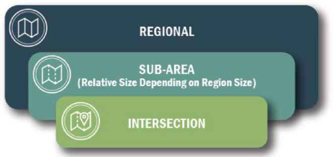
- region. The analysis models are usually microscopic in nature, and MOEs are typically associated with measures used by engineers (e.g., average speed, travel time, travel-time reliability). Typical corridor sections include a series of consecutive travel links on a major corridor as well as intersections, interchanges, parallel arterials (e.g., frontage roads), cross streets, and entrance/exit ramps.
- Regional level: For strategies that require larger networks to capture the full effects. The models are typically mesoscopic in nature to capture the regional effects of route choices and diversions given various network conditions and user classes (e.g., regular commuters and tourists). Mesoscopic models are node-and-link-based, so they are most useful when considering the transportation network at a system level. MOEs from regional models are usually consistent with measures used in regional planning [e.g., vehicle-miles traveled (VMTs), travel time reliability, diversion to/from facility].
Modeling Tools and ATM
Table 6-1 shows the applicability of the main modeling/simulation tools for different ATM strategies and levels of analysis (i.e., intersection, sub-area, or regional). The appropriateness of the various tools for each ATM strategy is further described as follows:
- Adaptive ramp metering: Microscopic models are best suited for adaptive ramp metering because they can use external scripting algorithms and a customized software interface to dynamically control the vehicle flow rate entering a freeway system. Mesoscopic models are also capable of simulating ramp metering at a corridor or regional level. Some signal optimization tools can also be applied to conduct corridor-level analyses.
- Adaptive traffic signal control: Microscopic simulation tools are needed to model adaptive traffic signal control optimization because they respond more intelligently to fluctuations in traffic patterns and vehicle detections and dynamically adjust cycle lengths, phase split times, and offsets. Micromodels can be managed with actual traffic data for adaptive traffic signal control; typically, an external source code or emulator is needed to simulate adaptive traffic signal control. Traffic signal optimization tools can also be used at a corridor level.
- Dynamic junction control: Microscopic models are best suited for merge and junction control. Micromodels (with the use of external scripting) can dynamically reallocate lane and/or ramp access by either increasing capacity or time-dependently closing roadway sections.
- Dynamic lane reversal: Both microscopic and mesoscopic simulation tools can be used to model the impacts of dynamic lane reversal. Microscopic models can be used to analyze how egress/ingress locations impact traffic flow. Mesoscopic models are capable of modeling dynamic lane reversal (e.g., contraflow lanes during hurricane evacuation) and are often
Table 6-1. Applicability of modeling tools for analysis of ATM strategies.
| ATM Strategy | Microscopic Simulation | Mesoscopic Simulation | Signal Optimization Tools |
|---|---|---|---|
| Adaptive Ramp Metering |  |  | |
| Adaptive Traffic Signal Control | | — | |
| Dynamic Junction Control | | — | — |
| Dynamic Lane Reversal |  | | — |
| Dynamic Lane-Use Control | | — | — |
| Part-Time Shoulder Use | | | — |
| Queue Warning | | | — |
| Transit Signal Priority | | — | |
| Variable Speed Limits | | | — |
| Intersection | Sub-area |  Regional Regional |
NOTE: — = not applicable.
- used to analyze the impacts of extent, scheduling, and operational strategies of dynamic lane reversal on directional traffic flow at a regional level (Hausknecht et al. 2011).
- Dynamic lane-use control: Microscopic simulation tools are appropriate for lane-use control because they model individual lanes and individual vehicles with high fidelity. Microscopic models allow for lane closure within the simulation time horizon and can be designed to activate/deactivate automatically in response to system detector inputs. Customized control strategies may need to be developed using external add-on scripting to simulate potential lane closures (Radwan et al. 2011).
- Part-time shoulder use: Microscopic models are best suited to analyze the impacts of vehicle interactions at merge/weave locations. Microscopic models can also determine the total
- increase in traffic flow on a corridor given additional capacity from part-time shoulder use. Mesoscopic models can also simulate part-time shoulder use at an aggregate level. Mesoscopic models do not simulate at the individual lane level but can show the impacts of the added capacity at a system-wide level. Calibration of capacity inputs is therefore critical to the simulation results of mesoscopic models (Coffey and Park 2020).
- Queue warning: Microscopic models can be used, typically in conjunction with VSLs, to analyze the immediate corridor-level impacts of queue warning systems. Scripting is needed to adjust speed limits when downstream queuing has disrupted traffic flow. The impacts are also sensitive to assumptions about driver compliance and behavioral responses to warning messages. Mesoscopic models can be used at a regional level to simulate detours of vehicles to alternative routes when bottleneck locations warrant a queue warning. Alternative route and diversion rates must also be defined.
- VSLs: Microscopic simulation tools are best suited for VSLs because they employ a time-step approach to track individual vehicles. Microscopic models allow speeds to be varied on various roadway sections and can be designed to activate/deactivate in response to traffic conditions. Unlike macroscopic models that are link-based, microscopic models are lane-based simulation tools that are capable of modeling various user classes at an individual vehicle level. Mesoscopic models can also be used to simulate traffic operational changes at the corridor or regional level (Khondaker and Kattan 2015).
ATM strategies can be modeled in conjunction with strategies tied to transit, such as transit signal priority. The level of tools that can support a more complex AMS framework to address multimodal strategies is identified as follows:
- Adaptive ramp metering: Microscopic or mesoscopic tools.
- Adaptive traffic signal control: Microscopic tools (typically one that is geared for traffic signals).
- Dynamic junction control: Microscopic tools (mesoscopic tools are not lane-based).
- Dynamic lane reversal or contraflow: Mesoscopic tools for regional contraflow, such as hurricane evacuation; microscopic or mesoscopic tools for regular lane reversal.
- Dynamic lane-use control: Microscopic tools (mesoscopic tools are not lane-based).
- Part-time shoulder use: Mesoscopic or microscopic tools.
- Queue warning: Mesoscopic or microscopic tools, with a possible need for additional scripting.
- VSL: Microscopic tools.
A series of tools and methods are needed to test the benefits of ATM and to encourage traffic operators and other agencies (decision-makers) to embrace the concept. These tools and methods will enable the user to evaluate the potential benefits of ATM strategies dynamically and proactively. An AMS framework is needed to help agencies evaluate ATM at the planning, design, and operational stages, as shown in Table 6-2 (Yelchuro et al. 2013).
Data Requirements

Applying an AMS framework to ATM strategies will require both historical and real-time data as inputs into the scenario manager, where the data are processed into standardized formats, and scenarios are developed. It is important to note that there may be instances where the data are inconsistent or in an incompatible format. In these instances, it is imperative that the data are standardized for integration with the scenario manager. Data are then used as inputs into the simulation-based environment where various scenarios are modeled. As part of the AMS framework, the user needs to make assumptions regarding how travelers would respond to control commands and advisory messages provided via the ATM strategies.
Table 6-2. Modeling applications.
| ATM Strategy | Planning | Design | Operations |
|---|---|---|---|
| Adaptive Ramp Metering | Identify predeployment infrastructure needs, perform cost analysis . | Use signal optimization to determine entry flow rates, storage space, and acceleration distance . | Use ramp metering to regulate operational inflow during peak/off -peak hours |
| Adaptive Traffic Signal Control | Identify predeployment infrastructure needs, perform cost analysis . | Help design roadway capacity, turning bays, storage lengths, and entry flow rates using algorithms. | Use adaptive traffic signal control to help reduce congestion levels on arterial corridors (through signal coordination); able to implement various adaptive traffic control algorithms. |
| Dynamic Junction Control | Identify predeployment infrastructure needs, perform cost analysis, plan for special events and long-term work zones . | Help design roadway capacity, part -time shoulder use, and work zone traffic flow . | Use junction control to dynamically allocate lane access to increase capacity and decrease time-dependent closures. |
| Dynamic Lane Reversal | Identify freeway/ arterial emergency management, incident management, special events, and long-term congestion implications. | Determine optimal location for when and where strategy is implemented and associated movable barrier/proper signage needs. | Analyze how contraflow lanes impact traffic (i.e., increase throughput) at the corridor (arterial) and regional (freeway) level; requires coordination with police/roadway officials. |
| Dynamic Lane-Use Control | Identify predeployment infrastructure needs, perform cost analysis, plan for special events and long-term work zones. | Determine optimal locations for dynamic lane control signs mounted over traffic. | Analyze how lane utilization impacts traffic flow; often used with VSLs. |
| Part-Time Shoulder Use | Plan for incident management and managed lanes . | Determine optimal ingress/egress locations and signage . | Analyze traffic flow during peak periods, including how the shoulder traffic merges back into main lanes. |
| Queue Warning | Identify predeployment infrastructure needs, perform cost analysis . | Determine optimal locations for DMS. | Broadcast message to alert motorists to queues or significant speed reduction areas. |
| Transit Signal Priority | Identify predeployment infrastructure needs, perform cost analysis . | Determine design and location of transit stops, transit-only lanes. | Use transit signal priority to improve speed and reliability of transit service by giving preferential treatment at intersections . |
| VSLs | Identify policy -related questions regarding speed reduction limits and time-of-day implementation . | Determine optimal locations for speed detectors. | Determine whether VSLs improve flow through the corridor. |
SOURCE: Adapted from Yelchuro et al. 2013.
Real-Time Data
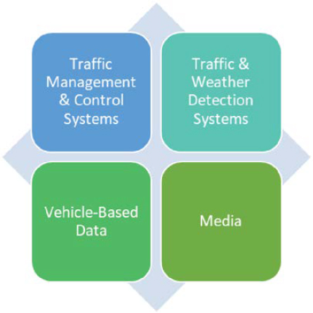
The AMS framework must be capable of modeling various tactical decisions as travelers execute their trips. These tactical decisions may be modeled by a range of models with varying degrees of precision and accuracy. The AMS framework needs to leverage real-time data to support analysis at the desired temporal and geographic scales. The AMS framework needs to support the ability to use real-time data in an integrated fashion either at the regional or corridor level for the desired analysis scale (e.g., peak period). Real-time data are derived from multiple sources, as shown in Figure 6-3, and are limited to use in simulation-based model applications at the micro, meso, and macro levels. For ATM analysis, sketch planning, travel demand, analytic/ deterministic models do not have a temporal profile and therefore are not capable of utilizing real-time data.
Traffic Management and Control Systems
Signaling and signage systems, such as ramp metering systems, traffic control systems, variable message signs, and static signage, are used to influence and control driver decision-making and can be fixed or autonomous. Components of traffic management and control systems include the following:
- Traffic control systems: Provide for the integration and adaptive control of the freeway and surface street networks to improve the flow of traffic, give preference to transit and other HOVs, and minimize congestion. These systems gather data from the transportation network, fuse it into usable information, and use it to determine the optimum assignment of right-of-way to vehicles and pedestrians. Examples of data from traffic control systems include the following:
- System control data: Data comprised of traffic signal control (e.g., signal timing/phases, algorithms for ramp metering adaptive control), available roadway capacity (e.g., lane restrictions, shoulder lane utilization), toll pricing structure, and work zone/incident characteristics.
- Closed-circuit television: Data comprised of vehicle occupancy counts and vehicle types.
- Detector data: Either sensor or video surveillance data comprised of lane-based counts (e.g., volume and speed data), typically in 5-minute intervals for both freeway and arterials.
- Transit data: Data comprised of transit schedules, headways, pricing, and operations (e.g., ridership).
- Route guidance: Provides travelers with a suggested route to reach a specified destination, along with simple instructions on upcoming turns and maneuvers (Zegeer et al. 2014).
- Agency activity: Summarizes the incident management and other operational aspects that affect the ATM project operation.
Vehicle-Based Data
Instrumented vehicles can serve as sensors providing real-time data sources for AMS applications. Examples of instrumentation include global positioning system devices and DSRC radio units, which are being developed as part of CV programs. The advances in technology and the increasing connectivity through wireless communication have made this type of data more feasible. Recent research has linked wireless communication data with traffic simulation models to replicate vehicle-to-vehicle and vehicle-to-infrastructure communication. The type of wireless communication used will be influenced by the availability of wireless infrastructure as well as the application objectives, which in turn will determine the capability to obtain real-time or near-real-time datasets for AMS.
For safety-oriented applications, the wireless communication will likely be low-latency DSRC. For nonsafety-critical applications, the choice of wireless media and its performance can vary greatly depending on the infrastructure architecture, geographical coverage, and network topology.
Examples of wireless data include car positions, speeds, acceleration/deceleration values, time gaps and headways, and predetermined destinations.
Media
Information broadcast by the media reaches system users over a large geographical area. Media information includes traffic reports delivered through commercial radio, highway advisory radio, television broadcasts, and pertinent information provided over the Internet (e.g., Google Maps displaying color-coded congestion maps representing speed profiles). The media can provide both pretrip and en route forms of data as follows:
- Pretrip information: Allows travelers to access a complete range of real-time multimodal transportation information at home, work, and other major sites where trips may originate. Information on the road network conditions, incidents, weather, and transit services are conveyed through these systems to provide travelers with the latest conditions and opportunities to plan their travel. Based on this information, the traveler can select the best departure time, route, and mode of travel, or perhaps not make a trip at all. Examples of pretrip information include forecasted travel times, incident locations, roadway closures (extent and duration), departure time impacts, and work zone locations (extent, duration, and timing).
- En route information: Includes driver advisories (via DMS/radio) conveying information about traffic conditions, incidents, construction, transit schedules, and other mode choice options to drivers and users of personal, commercial, and public transit vehicles. Examples of en route information include current travel times, toll rates, diversion routes, and congestion levels (expected duration).
Traffic and Weather Detection Systems
Systems that detect and classify elements of vehicle or pedestrian movement are dependent on traffic and/or weather-related data. Transportation operators are most interested in how weather conditions currently or are expected to interact in the future with pavement conditions. Types of weather-related data include visibility impairments (fog, rain, snow, dust, and smoke), precipitation (rain, snow, sleet), and pavement conditions by location. Automated weather observing system (AWOS) units are operated and controlled by the Federal Aviation Administration as well as by state and local governments and some private agencies. AWOS units report weather conditions at set intervals and typically cover precipitation, temperature, and barometric pressure. Well-integrated weather information allows traffic management center operators to make effective and timely management and operational decisions based on quality information related to weather observations and forecasts, the anticipated timing and intensity of weather events, the interaction of weather conditions with the road surface, and the type and availability of appropriate transportation management devices and systems (Vasudevan and Wunderlich 2013).
In general, cleaning, processing, integrating, visualizing, or using real-time data obtained from different sources can be quite challenging because the data may have different specifications, formats, and spatiotemporal resolutions. Recent research efforts have focused on addressing these needs. For example, the Florida DOT Research Center developed an integrated ITS data analysis tool that allows users to manage and condition data for use in transportation modeling, generate performance measurements of the transportation and ITS system, and discover new relationships and associations within the ITS data using data mining and visualization techniques (Hadi et al. 2012).
Historical Data
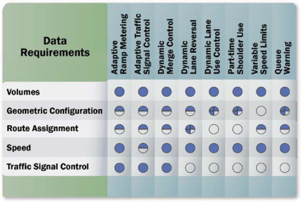
Historical data are used to populate the simulation-based model and are the foundation for the simulated environment. These datasets include speed and traffic volumes used for calibration, geometric design features and signal timings used for network setup and configuration, and OD and route assignment data used to determine the time-dependent shortest path. Examples of historical data used for AMS include the following:
- Volumes: Models typically use average annual daily traffic or average daily traffic to help validate the model’s highway assignment. Traffic counts are usually segregated by vehicle class (e.g., passenger cars versus trucks).
- Geometric configuration: Models normally include the number of lanes, lane merge/diverge areas, left-/right-turn bays, U-turns, facility types, and capacities.
- Route assignment: Regional-level models typically use OD matrices for route assignment. Traffic volumes are used for OD matrix estimation (ODME) and calibration. Smaller-scale (microscopic) models use static assignment routing where data on the defined path and turning movements are needed. If transit is included in a modeled network, then transit route stop and time-of-day schedule data are needed. Household income level data are needed for monetary facility choices (i.e., value of time).
- Speed: Data are expressed in networks as free-flow speeds, where vehicles can travel through the network without regard for congestion. Speeds are defined based on the functional class of the roadway (e.g., freeway free-flow speed is 60 mph).
- Traffic signal control: Data define the cycle length, green time, offsets, splits, and coordination. Ramp metering can be considered a signal control, and therefore flow rate is governed by congestion levels.
It is important to note that the segment-level, corridor-level, and regional-level data requirements have been consolidated, and historical data have been categorized based on distinct ratings, as shown in Figure 6-4.
Calibration and Validation
No model can reproduce reality perfectly, so it is important to develop models that achieve practicality and ensure that the model reflects travel behavior. Calibration is the adjustment of a model’s parameters to improve its ability to reproduce driver behavior and traffic performance characteristics. This step is necessary because no single model can accurately account for all possible traffic conditions and because models must be adapted to local conditions. It requires more time and effort due to a wide range of factors and inputs that influence the model results and output. It involves the adjustment of model parameters to improve its ability to accurately reflect existing as well as anticipated traffic conditions.
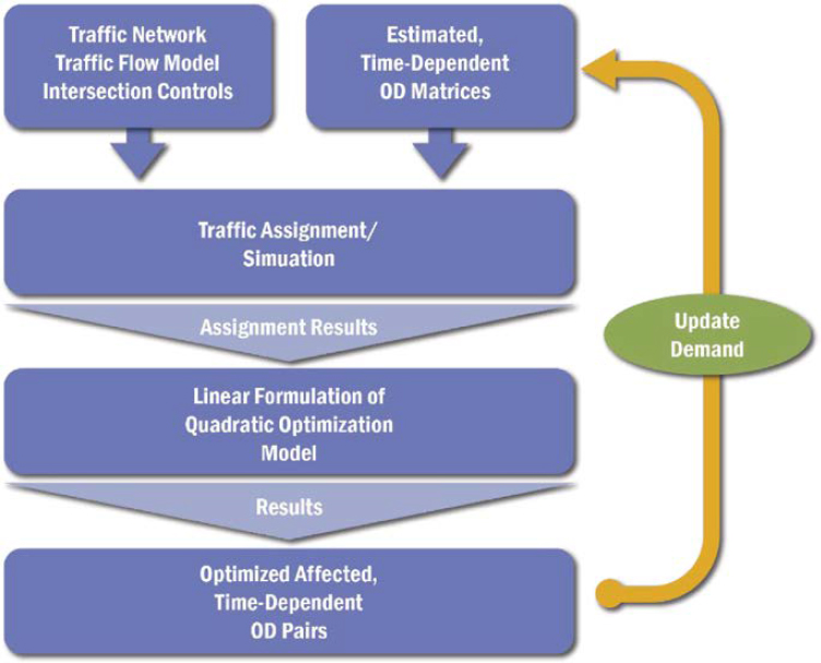
Calibration involves the adjustment of driver behavior parameters, route choice parameters, OD matrix estimates, control strategies, and overall model performance, as shown in Figure 6-5. A calibration objective function should be chosen, and the analyst should seek to minimize the
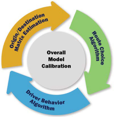
error between model output and field measurement. The general calibration objective function can be described as an optimization problem with the objective of minimizing the relative gap measure by comparing the observed and fitted measurement values. The relative gap may be used to quantify a given solution and can be defined as the difference between the total travel time experienced and the total travel time that would have been experienced if all vehicles had a travel time equal to that of the current shortest path.
It should be noted that model development is a tedious process and that network coding errors are a major source of abnormal vehicular movements. Such errors can be found at any time during the calibration process. Accordingly, fixing network coding errors is an important task throughout the entire calibration process.
Driver Behavior Algorithms
Driver behavior can be captured using car-following and lane-changing algorithms, which govern vehicular traffic movement. The parameters of these algorithms need to be adjusted for a specific region. Global parameters within a windowed subnetwork level using either disaggregated or aggregated data are as follows (Chu et al. 2004):
- Car-following parameters:
- Look-ahead distance.
- Look-back distance.
- Headway time/gap acceptance.
- Acceleration/deceleration.
- Average stopped distance.
- Driver reaction time.
- Right-of-way constraints.
- Lane-changing parameters:
- Minimum front/rear headways.
- Desired position during free-flow conditions.
- Lane-changing distance.
- Network parameters:
- Speed profiles.
Route Choice Algorithms
Route choice behavior is another aspect of network calibration wherein the drivers have more than one viable route choice. Field data to capture route choice can rarely be obtained; an inappropriate route choice parameter value can annul the accurate calibration of all other parameters. Adjusting the route choice behavior parameters must be conducted on a network-wide level using either aggregated data or individual data obtained from driver surveys (Kunde 2002). Many regional simulation-based, dynamic traffic assignment models employ some sort of traffic flow model that moves vehicles according to their speed-density (v-k) relationship using traffic counts (converted to flows) and average speeds at defined time intervals. Data are typically collected using tube counters, third-party data collection, or existing freeway sensors. Typical statistical metrics determining the goodness-of-fit of the simulated measures can be used, such as a linear regression model. In a mesoscopic modeling framework, vehicles move according to the v-k relationship. The v-k relationship can be calibrated using typical tube counter data in which the average speeds and counts are plotted per user-defined interval.
ODME
Calibration of an OD matrix involves several substeps, if applicable (see Figure 6-6). (Segment-level models do not require an OD matrix; routes are usually defined as static and are generally defined by the analyst.) While there are many different types of ODMEs aimed at calibrating trip tables, they all employ some sort of optimization algorithm to minimize the standard deviation between simulated and field data. Typically, this type of calibration is an iterative process that calls for the optimization of screen line and simulated counts and adjusts all OD pairs that travel through all sections of the roadway where data are collected. It must be noted that the route choice algorithm and ODME work in tandem, where new route choices are updated during each simulation iteration (Chiu 2014). It must also be noted that most travel demand models employ some sort of seed OD matrix; the flows it produces on surrounding roadways typically do not match counts collected in the field. An ODME process helps the models produce a more realistic representation of traffic conditions. An ODME can be developed for individual or multiple vehicle classes.
Validation is the process where the analyst checks the overall predicted model outputs, such as traffic volumes, average speeds, door-to-door travel times, and average delays. Ideally, model validation is performed based on data collected in the field but not used in calibration. A good validation test shows the predicted/simulated values within ±10 percent of the actual field data.
Performance Measures
Once a model has been properly calibrated and validated, a base model is developed and used as a basis for comparison. Alternate scenarios can then be developed and simulated to obtain various performance measures and generate the appropriate output.
Literature reveals a plethora of performance measures that can be computed depending on the ATM strategy of interest and the software package used to model it. Most of the MOEs reported in the past have been derived from the following basic metrics: travel time, speed, volume, delay, queue, stops, and density. If these measures are determined, one can take the following actions (Dowling 2007):
- Compute other commonly used metrics or indicators of performance such as HCM LOS, volume/capacity ratio (V/C), VMT, vehicle-hours traveled, person-miles traveled, lateral and longitudinal speed differential, duration of speed less than a specified threshold, flow/speed plot, speed contour diagram, headway distribution, vehicle hour delay, and so forth.
- Conduct B/C analyses and estimate other measures that pertain to economic and comprehensive costs, air quality, noise, and energy use such as emissions, fuel consumption, and noise level.
Table 6-3 shows the main measures of effectiveness that are typically computed when analyzing ATM strategies at a corridor level. It is worth noting that depending on the objectives of the analysis and the ATM strategy selected, some MOEs may be more appropriate than others, making their use more or less significant and meaningful.
Speed and travel time are interchangeable measures, although travel time best reflects what travelers and shippers value. Calculating the percentage change in speed, for example, will not give an accurate portrayal of the change in travel time. Travel time expresses the amount of time spent by travelers to complete a trip within a segment, corridor (corridor level), or network (regional level).
Volume or throughput is the number of vehicles present at the start plus those vehicles attempting to enter and successfully entering the system during the analysis period. It can be estimated from demand and capacity. When downstream volumes are computed, one should take into consideration upstream capacity constraints. Most of the other metrics can be derived
Table 6-3. Performance measures per ATM strategy for corridor-level analysis.
| Measures of Effectiveness (MOEs) | Adaptive Ramp Metering | Adaptive Traffic Signal Control | Dynamic Junction Control | Dynamic Lane Reversal | Dynamic Lane-Use Control | Part-Time Shoulder Use | Queue Warning | Transit Signal Priority | Variable Speed Limits |
|---|---|---|---|---|---|---|---|---|---|
| Speed | X | X | X | X | X | X | — | X | X |
| Travel Time | X | X | X | X | X | X | X | X | X |
| Volume or Throughput | X | X | X | X | X | X | — | X | X |
| Delay | X | X | — | X | X | X | X | X | X |
| Number of Stops | — | X | — | — | — | — | — | X | — |
| Queue Length | X | X | — | — | — | — | X | — | — |
| Reliability Measures | X | — | — | X | X | X | X | X | X |
| Acceleration/Deceleration | — | — | — | — | — | — | — | X | X |
| HCM LOS | X | X | X | X | X | X | — | — | X |
| V/C | — | — | — | — | X | X | — | — | X |
| Emissions/Noise/Fuel Consumption | X | X | — | — | — | — | — | X | — |
NOTE: — = not applicable.
from speed, travel time, and volume. Note that capacity is also one of the main traffic parameters and a basic characteristic of a facility (Dowling 2007).
Delay may have different forms such as stop, control, and approach delay. Stop delay is the time a vehicle is stopped in a queue while waiting to pass through the intersection, while the average stopped-time delay is the average for all vehicles during a specified period. Control delay is typically caused by downstream control devices, traffic signals, or stop signs. Approach delay includes stopped-time delay but adds the time loss due to deceleration from the approach speed to a stop and the time loss due to re-acceleration back to the desired speed. The number of stops is often an input parameter in signal timing optimization algorithms and can be used to compute other measures.
Queue length is an indicator of hot-spot locations within the system where capacity inefficiencies and/or safety problems may exist due to intersection blockages or turn bay overflows (Dowling 2007).
Travel-time reliability reflects the distribution of trip travel times across a facility over an extended period (Zegeer et al. 2014). This distribution arises from the interaction of several factors that influence travel times. Some of these factors include recurring variations in demand, severe weather conditions, incidents, work zones, and other special events. Chapter 36—“Travel Time Reliability” of the HCM (HCM7 2022) provides methodologies for incorporating travel time reliability into the analytic procedures for freeway facilities and urban streets.
The HCM provides a list of measures that can be used to quantify differences in reliability between facilities and evaluate alternatives to improve reliability (Zegeer et al. 2014). Some measures describe typical (average) conditions, which are evaluated by a standard HCM freeway or urban facility analysis. Measures for these conditions include travel time (min), 50th percentile travel-time index, and annual delay (veh/hr and people/hr). Other measures describe travel time variability or the success/failure of individual trips in meeting a target travel time or speed. These measures include the following:
- Planning time index (PTI): Unitless measure that reflects how much time a traveler should allow to complete a trip on time in relation to the time for the same trip in low-volume (free-flow) conditions (Margiotta et al. 2006).
- Eightieth percentile travel-time index: Unitless measure that is more sensitive to operational changes than the PTI, thus making it useful for comparison and prioritization purposes.
- Failure/on-time measures: Percentage (from 0 to 100 percent) of trips with space mean speeds above (on time) or below (failure) one or more target values.
- Reliability rating: Percentage (from 0 to 100 percent) of trips experiencing a travel-time index less than 1.33 for freeways and 2.50 for urban streets.
- Semi-standard deviation: Unitless measure that provides the variability distance from free-flow conditions and is a one-sided standard deviation with the reference point at free-flow speed instead of the mean.
- Standard deviation: Unitless standard statistical measure.
- Misery index: Unitless measure that is useful as a descriptor of near-worst-case conditions on rural facilities.
Acceleration/deceleration fluctuations are good indicators of whether a freeway facility is flowing at a constant and uniform speed. Disturbances to the system (e.g., incidents; heavy inflow from ramps; slower, heavy vehicles) can cause shockwaves and disrupt flows on the facility. Also known as speed harmonization, this measure is a good indicator of the overall performance of the transportation system.
The HCM LOS captures the quality of traffic service within a facility. The method of determining the LOS involves creating categories of traffic flow and assigning quality levels of traffic
Table 6-4. Building blocks of performance measurement systems.
| MOE | Typical Usage |
|---|---|
| Travel Time |
|
| Speed |
|
| Delay |
|
| Queue |
|
| Stops |
|
| Density |
|
| HCM LOS |
|
| V/C |
|
SOURCE: Adapted from Zegeer et al. 2014.
based on performance measures, such as speed and density. The V/C is another HCM performance measure that indicates the level of traffic operating conditions.
Emissions, noise, and fuel consumption are estimated from other basic measures such as stops, speed, and delay (Dowling 2007).
In addition to the MOEs listed above, crash rates and number of injuries by severity are other measures that reflect how traffic safety is affected by ATM strategies. These metrics are separately estimated and compared for the period before and after the implementation of a strategy. However, these safety metrics are not directly calculated or provided by commonly used simulation/modeling tools. This omission is an undiscovered area that the majority of the existing simulation/modeling tools do not address. Table 6-4 shows the main application areas of the most widely used MOEs.
Table 6-5 shows the measures that are typically needed to evaluate the performance of different ATM strategies at a corridor level. Like the corridor-level analysis (Table 6-3), some metrics may be more useful than others, depending on the objectives of the analysis and the ATM strategy selected. Note that some performance measures used in a corridor-level analysis (e.g., LOS) cannot be calculated for a regional-level analysis and vice versa (e.g., system delay).
Final Remarks
The AMS framework is a powerful tool for planning and evaluating ATM strategies in transportation systems during the planning and implementation processes. AMS provides an analytical framework for assessment throughout the planning and implementation process.
Table 6-5. Performance measures per ATM strategy for regional-level analysis.
| Measures of Effectiveness (MOEs) | Adaptive Ramp Metering | Adaptive Traffic Signal Control | Dynamic Junction Control | Dynamic Lane Reversal | Dynamic Lane-Use Control | Part-Time Shoulder Use | Queue Warning | Transit Signal Priority | Variable Speed Limits |
|---|---|---|---|---|---|---|---|---|---|
| Average Speed | X | X | X | X | X | X | X | X | X |
| Volume or Throughput | X | — | X | X | X | X | X | X | X |
| Density | — | — | X | X | X | X | — | — | X |
| System Delay | X | X | X | — | X | — | X | — | X |
| Number of Stops | X | X | — | — | — | — | — | X | — |
| Queue Length | — | X | — | — | — | — | X | X | — |
| Total System Travel Time | X | X | X | X | X | X | X | X | X |
| Reliability Measures | X | X | — | — | X | X | — | X | X |
| Average V/C | X | X | X | — | X | X | — | — | — |
| Emissions/Noise/Fuel Consumption | X | X | — | — | — | — | — | X | — |
NOTE: — = not applicable.
It helps various agencies and stakeholders evaluate ATM strategies at the planning, design, and operational stages. Using these tools and assets, operating agencies manage traffic flow and influence driver behavior in real time to achieve operational objectives. This chapter highlights the AMS framework, including the types of modeling tools, data requirements, calibration and validation, performance measures, and final remarks, all related to the analysis, modeling, and simulation of ATM. This framework can guide the ATM assessment process by providing an overview of the analysis, modeling, and simulation tools and methods that can be used to test and evaluate the effectiveness of active ATM strategies for agencies considering deployment.
Chapter 6 References
Chiu, Y.-C. (2014). “DynusT Online User’s Manual.” https://www.dynust.com/. Accessed May 2023.
Chu, L., H.X. Liu, J.-S. Oh, and W. Recker. (2004). “A Calibration Procedure for Microscopic Traffic Simulation.” Paper presented at the 2004 Annual Meeting of the Transportation Research Board, Washington, DC.
Coffey, S., and S. Park. (2020). “Part-Time Shoulder Use Operational Impact on the Safety Performance of Interstate 476.” Traffic Injury Prevention, Volume 21, Issue 7, 470–475. https://www.sciencedirect.com/org/science/article/abs/pii/S1538958822003356. Accessed May 2023.
Dowling, R. (2007). Traffic Analysis Toolbox Volume VI: Definition, Interpretation, and Calculation of Traffic Analysis Tools Measures of Effectiveness. Federal Highway Administration, U.S. Department of Transportation. Publication FHWA-HOP-08-054. https://rosap.ntl.bts.gov/view/dot/42195. Accessed May 2023.
Hadi, M., Y. Xiao, C. Zhan, and P. Alvarez. (2012). Integrated Environment for Performance Measurements and Assessment of Intelligent Transportation Systems Operations. Florida Department of Transportation. Draft Final Report, Contract No. BDK80 977-11. https://rosap.ntl.bts.gov/view/dot/24908. Accessed May 2023.
Hausknecht, M., T.-C. Au, P. Stone, D. Fajardo, and T. Waller. (2011). “Dynamic Lane Reversal in Traffic Management.” Proceedings of the 14th IEEE ITS Conference. https://nacto.org/wp-content/uploads/2015/04/dynamic_lane_reversal_hausknecht.pdf. Accessed May 2023.
HCM7. (2022). Highway Capacity Manual: A Guide for Multimodel Mobility Analysis, 7th ed. Transportation Research Board, Washington, DC.
Jacobson, J., J. Stribiak, L. Nelson, and D. Sallman. (2006). Ramp Management and Control Handbook. Federal Highway Administration, U.S. Department of Transportation. Publication FHWA-HOP-06-001. https://ops.fhwa.dot.gov/publications/ramp_mgmt_handbook/manual/manual/index.htm. Accessed May 2023.
Jeannotte, K., A. Chandra, V. Alexiadis, and A. Skabardonis. (2004). Traffic Analysis Toolbox Volume II: Decision Support Methodology for Selecting Traffic Analysis Tools. Federal Highway Administration, U.S. Department of Transportation. Publication FHWA-HRT-04-039. https://ops.fhwa.dot.gov/trafficanalysistools/tat_vol2/Vol2_Methodology.pdf. Accessed May 2023.
Khondaker, B., and L. Kattan. (2015). “Variable Speed Limit: A Microscopic Analysis in a Connected Vehicle Environment.” Transportation Research Part C: Emerging Technologies, Volume 58, Part A, 146–159. https://doi.org/10.1016/j.trc.2015.07.014. Accessed May 2023.
Kunde, K. K. (2002). Calibration of Mesoscopic Traffic Simulation Models for Dynamic Traffic Assignment. Master’s Thesis. Massachusetts Institute of Technology.
Margiotta, R, T. Lomax, M. Hallenbeck, S. Turner, A. Skabardonis, C. Ferrell, and B. Eisele. (2006). NCHRP Web-Only Document 97: Guide to Effective Freeway Performance Measurement. Transportation Research Board, Washington, DC. https://www.trb.org/main/blurbs/158642.aspx. Accessed May 2023.
Möller, D., and B. Schroer. (2014). Introduction to Transportation Analysis, Modeling and Simulation, Simulation Foundations, Methods, and Applications. Springer, London, England.
Radwan, E., Z. Zaidi, and R. Harb. (2011). “Operational Evaluation of Dynamic Lane Merging in Work Zones with Variable Speed Limits.” In 6th International Symposium on Highway Capacity and Quality of Service, Procedia-Social and Behavioral Sciences, Volume 16, Issue 1–3. 460–469. https://www.sciencedirect.com/journal/procedia-social-and-behavioral-sciences/vol/16. Accessed May 2023.
Vasudevan, M., and K. Wunderlich. (2013). Analysis, Modeling, and Simulation (AMS) Testbed Framework for Dynamic Mobility Applications (DMA) and Active Transportation and Demand Management (ATDM) Programs. Federal Highway Administration, U.S. Department of Transportation. Publication FHWA-JPO-13-095. https://rosap.ntl.bts.gov/view/dot/3405. Accessed May 2023.
Waller, T., M.-W. Ng, E. Ferguson, N. Nezamuddin, and D. Sun. (2009). Speed Harmonization and Peak-Period Shoulder Use to Manage Urban Freeway Congestion. Texas Department of Transportation. Publication FHWA/TX/0-5913-1. https://rosap.ntl.bts.gov/view/dot/17942. Accessed May 2023.
Yelchuru, B., S. Singuluri, and S. Rajiwade. (2013). Active Transportation and Demand Management (ATDM) Foundational Research: Analysis Plan. Intelligent Transportation Systems Joint Program Office, U.S. Department of Transportation. Publication FHWA-JPO-13-022. https://rosap.ntl.bts.gov/view/dot/3381. Accessed May 2023.
Zegeer, J., J. Bonneson, R. Dowling, P. Ryus, M. Vandehey, W. Kittelson, N. Rouphail, B. Schroeder, A. Hajbabaie, B. Aghdashi, T. Chase, S. Sajjadi, R. Margiotta, and L. Elefteriadou. (2014). SHRP 2 Report S2-L08-RW-1: Incorporating Travel Time Reliability into the Highway Capacity Manual. Transportation Research Board of the National Academies, Washington DC. https://www.trb.org/Publications/Blurbs/169594.aspx. Accessed May 2023.


