Airport Curbside and Terminal Area Roadway Operations: New Analysis and Strategies, Second Edition (2024)
Chapter: Appendix C: Overview of the Curbside Analysis Methodology in the Quick Analysis Tool for Airport Roadways (QATAR)
APPENDIX C
Overview of the Curbside Analysis Methodology in the Quick Analysis Tool for Airport Roadways (QATAR)
Queuing Model Structure
The basic assumptions used in developing the Quick Analysis Tool for Airport Roadways (QATAR) curbside queuing model are presented in the following. Several excellent texts on queuing theory are recommended for further reading on this topic (Hillier and Lieberman 2015, Newell 1982). The field of queuing theory is well developed, with standardized terminology. This section introduces the standard queuing theory terminology and assumptions used in constructing the QATAR model.
A queuing system consists of a facility providing some form of service to a defined population. The key values used to define a queuing system are the arrival rate, service time, number of servers, system capacity, calling population, and queue discipline. The time between arrivals (inter-arrival time or arrival rate) of members into the queuing system is modeled as a probability distribution.
The roadway in front of the airport terminal represents the service facility. It is modeled as a multiserver facility, with each curbside space considered a server. The system capacity is assumed to be infinite. The size of the population can be either finite or infinite, but for analytical models, it is usually defined as infinite because of the difficulty of deriving analytical solutions for finite systems. The queue discipline is specified as first-in-first-out.
Queuing models have assumptions and restrictions on their application. Queuing models are derived assuming steady-state conditions. For example, at some airports, there are relatively few early morning flights and consequently few vehicles driving through the terminal curbside area. The system is in a transient state, and queues form and disappear quickly or sporadically. As more flights begin to depart (or arrive), there is a steady flow of vehicles in and out of the terminal area, and the condition during those times is more analogous to a steady-state condition. Another restriction for queuing models is that the utilization factor ρ must be less than 1. The utilization factor is defined as ρ = λ/(sµ), where λ is the mean arrival rate of customers, s is the number of servers in the service facility, and µ is the mean service rate of the overall system. For any model, if the mean arrival rate, λ, is greater than the mean service rate, µ, the queue would grow indefinitely.
It is well documented in operations research literature and commonly assumed in transportation applications that customers randomly arriving at a service facility have an arrival pattern that is assumed to be a Poisson distribution process. The assumption of a Poisson arrival process results in an exponential inter-arrival time distribution. Assuming an exponential service rate for an airport terminal curbside is also realistic because drop-off and pickup times vary around a mean value due to variations in how long it takes to complete the loading/unloading process (number of passengers, amount of luggage, etc.).
Based on the above, the curbside can be modeled by a multiserver queuing system with a Poisson arrival process, a mean service rate that follows an exponential probability distribution, and an infinite calling population (an M/M/s model in queuing theory terminology). If the queue discipline is first-in-first-out, the analytical results for the basic outputs are given in Equation C-1 through Equation C-9 (Hillier and Lieberman 2015):
| (C-1) |
| (C-2) |
| (C-3) |
| (C-4) |
| (C-5) |
| (C-6) |
| (C-7) |
| (C-8) |
| (C-9) |
where
| s = | number of servers in the service facility |
| λ = | mean arrival rate of customers |
| vi = | flow rate of vehicle type i |
| µ = | mean service rate of the overall system |
| Di = | dwell time of vehicle type i |
| ρ = | utilization factor |
| Lq = | number of customers in the queue |
| L = | number of customers in the queuing system, equal to the customers in the queue plus the customers being served |
| Wq = | expected waiting time in the queue |
| W = | expected waiting time in the queuing system |
| Pn = | probability that exactly n customers are in the queuing system |
Inputs and Intermediate Calculations
1. Curbside Configuration
The curbside may be specified using one of the following configurations:
- Active: In this configuration, the curbside is used for loading and unloading along its entire length, with drivers assuming any available space. QATAR models these operations using curbside capacity and through-lane capacity models.
- Crosswalk: Crosswalks may be uncontrolled, controlled by active warning devices, or controlled by a traffic control signal. Flagging operations can be approximated using a traffic control signal. QATAR models these operations using crosswalk capacity models.
- Source/Sink: These are curbside segments of zero length that reflect any entrance or exit volumes between segments.
- Taxi/Transportation Network Company (TNC) queue: These are curbside segments used by taxi queues or by TNC vehicles operating with a PIN system. QATAR does not model operations of these types of queuing systems, as they are typically actively managed and fed from an offsite hold lot.
- Other: These curbside segments are used by vehicles providing service to disabled passengers, service vehicles, emergency vehicles, or other types. QATAR does not model operations of these types of segments.
2. Hourly Vehicle Arrival Rate
The number of vehicles arriving at the zone per hour is the sum of the volume of all vehicle types approaching zone z, as given in Equation C-10.
| (C-10) |
where
| WtdVehicleArrivalRatez = | weighted vehicle arrival rate for zone z [veh/h] |
| vz,i = | flow rate of vehicle type i in zone z [veh/h] |
3. Number of Equivalent Servers per Zone
The available curbside length divided by the average vehicle stall length provides an estimate of the number of equivalent servers in each lane within a zone. The number of equivalent servers multiplied by the number of available lanes provides an estimate of the total number of equivalent servers per zone. Because drivers may choose to park in lanes not intended for loading or unloading (e.g., by double-parking or triple-parking), the calculation of equivalent servers uses the total number of lanes on the roadway. These are given in Equation C-11 through Equation C-13.
| (C-11) |
| (C-12) |
| DerivedNoOfServersz = NumberOfLanesz * CurblaneCapacityz | (C-13) |
where
| WtdVehicleLengthz = | weighted vehicle length for zone z [ft/veh] |
| ParkingLengthi = | parking length of vehicle type i [ft] |
| vz,i = | flow rate of vehicle type i in zone z |
| CurblaneCapacityz = | curb lane capacity for zone z [veh] |
| CurbFrontagez = | length of curb frontage for zone z [ft] |
| DerivedNoOfServersz = | equivalent parking spaces (servers) for zone z |
| NumberOfLanesz = | total number of lanes (through and parking) for zone z |
4. Service Rate
The service rate is computed as the weighted dwell time, as shown in Equation C-14 and Equation C-15. QATAR allows the modeling of individual vehicle types. In such a situation, the service rate is equal to the dwell time assumed for the specific vehicle type.
| (C-14) |
| (C-15) |
where
| EstimatedServiceRatez = | vehicle service rate for zone z [veh/h] |
| WtdDwellTimez = | weighted dwell time zone z [min/veh] |
| Di = | dwell time of vehicle type i [min/veh] |
| vz,i = | flow rate of vehicle type i in zone z [veh/h] |
| WtdVehicleArrivalRatez = | weighted vehicle arrival rate for zone z [veh/h] |
5. System Utilization Factor
The system utilization factor is determined by Equation C-16. This factor is used to determine the overall ability of the system to serve demand and is a core assumption of the queuing calculation method. A system utilization factor greater than 1 will result in an error message in QATAR. In such a situation, the number of vehicles attempting to load and/or unload exceeds the number of servers in a zone (i.e., every lane is fully occupied by vehicles attempting to load and/or unload).
| (C-16) |
where
| SystemUtilFactorz = | system utilization factor for zone z |
| WtdVehicleArrivalRatez = | weighted vehicle arrival rate for zone z |
| EstimatedServiceRatez = | estimated service rate for zone z |
| DerivedNoOfServersz = | equivalent parking spaces (servers) for zone z |
6. Number of Vehicles in System Within a Zone
Using the results from the previously presented equations and the assumptions inherent to the queuing model, it is possible to estimate the probability of having n vehicles in the system.
In this model, probabilities are computed for values of n from 0 vehicles to 170 vehicles using Equation C-17 and Equation C-18 (Stewart 2009). The mathematical structure here is slightly different from that presented earlier but can be demonstrated to be mathematically equivalent.
| (C-17) |
| (C-18) |
where
| s = | number of servers in the service facility |
| λ = | mean arrival rate of customers |
| µ = | mean service rate of the overall system |
| Pn = | probability that exactly n customers are in the queuing system |
QATAR then incrementally calculates a cumulative density function using the sum of the probabilities from zero to n. The 95th percentile from the cumulative density function, Pcntile95CarsInSysz, is an estimate of the maximum number of vehicles in the system 95 percent of the time; this value is used to determine the performance of the curbside for zone z.
7. Curbside Utilization Ratio
Parking activity in each lane is estimated based on the curbside utilization ratio. The curbside utilization ratio is calculated by comparing the total length of vehicles assumed to be parked within a zone simultaneously (based on the 95th percentile from the cumulative distribution function for that zone) with the curbside length available for parking in that zone, as shown in Equation C-19. This ratio is a measure of the use of a given parking space within a curb segment and typically ranges from zero to 3, with the latter suggesting the use of double-parking and triple-parking at the same curb segment. This equation is a practical estimate that compares a practical, design-level demand with the capacity of the curb lane; it differs from the system utilization factor described previously that determines the overall applicability of the macroscopic queuing model.
| (C-19) |
where
| CurbUtilRatioz = | curbside utilization ratio for zone z |
| Pcntile95CarsInSysz = | 95th-percentile number of vehicles in system for zone z |
| CurblaneCapacityz = | curb lane capacity for zone z [veh] |
8. Percent Occupancy in Lanes 1, 2, and 3
The model uses two inputs to determine the tendency for drivers to double-park and triple-park. If the zone only has three total lanes, the model assumes that parking only occurs in the first and second lanes.
The model includes two parameters: TLane2, the proportion of the first lane that is filled before drivers start to park in the second lane, and TLane3, the proportion of the second lane that is filled before drivers start to park in the third lane. These parameters have a built-in default value for both inputs of 80%, which means that drivers park in the first lane until 80% of the first lane is occupied and that drivers will park in the third lane once 80% of the second lane is occupied. These values are approximations based on observations at multiple airports with multiple attraction points (e.g., doors, skycap positions) within one curbside zone. Due to the approximations used for estimating throughput capacity (discussed in the following), further refinement of these default values is unlikely to improve overall planning estimates. If more precision is needed, simulation is recommended.
For curbside zones with four or five total lanes, the percent occupancy of lanes 1, 2, and 3 used for parking (P1,z, P2,z, and P3,z) is calculated for each zone z as shown in Table C-1.
For curbside zones with three total lanes and double-parking allowed, P1,z and P2,z are calculated for each zone z as shown in Table C-2.
For curbside zones with three total lanes, one parking lane, and double-parking prohibited, P1,z and P2,z are calculated for each zone z as shown in Table C-3.
Table C-1. Percent occupancy by lane for four or five total lanes, double-parking allowed.
| Condition | Equations |
|---|---|
| CurbUtilRatioz ≤ TLane2 | P1,z = CurbUtilRatioz |
| TLane2 < CurbUtilRatioz ≤ (1 + TLane3); | P1,z = TLane2 + (CurbUtilRatioz – TLane2)/2 |
| P1,z ≤ 1.0 | P2,z = (CurbUtilRatioz – TLane2)/2 |
| TLane2 < CurbUtilRatioz ≤ (1 + TLane3); | P1,z = 1 |
| P1,z > 1.0 | P2,z = CurbUtilRatioz – 1 |
| CurbUtilRatioz > (1 + TLane3); | P1,z = 1 |
| P2,z ≤ 1.0 | P2,z = (CurbUtilRatioz – 1) + (CurbUtilRatioz – (1 + TLane3))/2 P3,z = (CurbUtilRatioz – (1 + TLane3))/2 |
| CurbUtilRatioz > (1 + TLane3); | P1 = 1 |
| P2,z > 1.0 | P2 = 1 P3 = CurbUtilRatioz – 2 |
Table C-2. Percent occupancy by lane for three total lanes, double-parking allowed.
| Condition | Equations |
|---|---|
| CurbUtilRatioz ≤ TLane2 | P1,z = CurbUtilRatioz |
| CurbUtilRatioz > TLane2; P1,z ≤ 1.0 | P1,z = TLane2 + (CurbUtilRatioz – TLane2)/2 P2,z = (CurbUtilRatioz – TLane2)/2 |
| CurbUtilRatioz > TLane2; P1,z > 1.0 | P1,z = 1 P2,z = CurbUtilRatioz – 1 |
Table C-3. Percent occupancy by lane for three total lanes, one parking lane, double-parking prohibited.
| Condition | Equations |
|---|---|
| CurbUtilRatioz ≤ 1 | P1,z = CurbUtilRatioz P1,z = 1 |
| CurbUtilRatioz > 1 | P2,z = CurbUtilRatioz – 1 |
The total number of vehicles in each lane is calculated using Equation C-20 through Equation C-22.
| NoOfVehiclesInCurbsideLanez = P1,z * CurblaneCapacityz | (C-20) |
| NoOfVehiclesDoubleParkedz = P2,z * CurblaneCapacityz | (C-21) |
| NoOfVehiclesTripleParkedz = P3,z * CurblaneCapacityz | (C-22) |
9. Curbside Sufficiency
The curbside sufficiency is based on comparing the curbside utilization ratio for each zone z to the thresholds given in Table C-4. These thresholds vary based on whether double-parking is allowed or prohibited.
10. Roadway Capacity
The roadway capacity, or through-lane capacity, of an airport curbside roadway is affected by curbside activity (i.e., vehicles stopping to load or unload passengers). As the curbside lanes become more congested, double-parking and potentially triple-parking will begin to block the roadway through lanes. Roadway capacity decreases continuously as curbside utilization increases. The decrease is more prominent when curbside activity reaches a level at which additional lanes are blocked, producing a non-linear slope to the curves. Capacity data are difficult to obtain due to the need for representative capacity conditions, which includes as a prerequisite a persistent queue upstream of the curbside section. In such cases, the roadway capacity is assumed to be the throughput on the roadway, measurable by standard industry traffic counting techniques.
Due to the significant downturn in air travel during the COVID-19 pandemic during the research for this project, no additional field data were collected. The research team used a limited amount of field data collected previously from the original research for ACRP Report 40, including data from Washington Dulles International Airport (IAD), San Francisco International Airport (SFO), and Oakland International Airport (OAK). To supplement the sparse field data available, the research team developed a VISSIM model to determine the curbside volume stopping in the parking lanes, which corresponds to various curbside utilization levels. By holding that level of curbside activity constant and increasing through traffic volumes during multiple simulation tests, the research team observed a progressive collapse of traffic flow, with a queue forming upstream of the curbside section. When the queue became persistent or continuously increasing, the roadway section was said to have reached capacity. The resulting throughput downstream of the modeled segment represents the capacity under those conditions. In addition, the research
Table C-4. Curbside sufficiency definitions.
| Curbside Utilization Ratio for Zone z, CurblaneCapacityz | Curbside Sufficiency |
|---|---|
| Double-Parking Allowed | |
| <= 1.30 > 1.30 to <= 1.70 > 1.70 to <= 2.00 > 2.00 |
Under Capacity Near Capacity At Capacity Over Capacity |
| Double-Parking Prohibited | |
| <= 1.00 > 1.00 to <=1.20 > 1.20 to <=1.35 > 1.35 |
Under Capacity Near Capacity At Capacity Over Capacity |
team applied considerable judgment in fitting the curves, based on experiences at airports throughout the United States and in other countries, including knowledge of the typical parking patterns around key features such as door locations.
The resulting complex, non-linear interactions can be described by the curves shown in Figure C-1. As noted previously, these curves were developed using a combination of the microsimulation testing of hypothetical airport curbsides, actual but limited field observations, and research team judgment.
The curves in Figure C-1 are mathematically represented as follows in Equation C-23, with constants for various configurations given in Table C-5:
| (C-23) |
where
| RdwyThruCapacityz = | roadway through capacity for zone z |
| CurbUtilRatioz = | curbside utilization ratio for zone z |
| ConstA, ConstB, ConstC, ConstD = | constants as given in Table C-5 |
Because model inputs are given in terms of driver’s side parking, through lanes, and passenger’s side parking, QATAR maps these configurations into one of the modeled configurations specified by total and approach lanes, as shown in Table C-6. Any configurations not included in Table C-6 are flagged to the user as not being supported by QATAR.
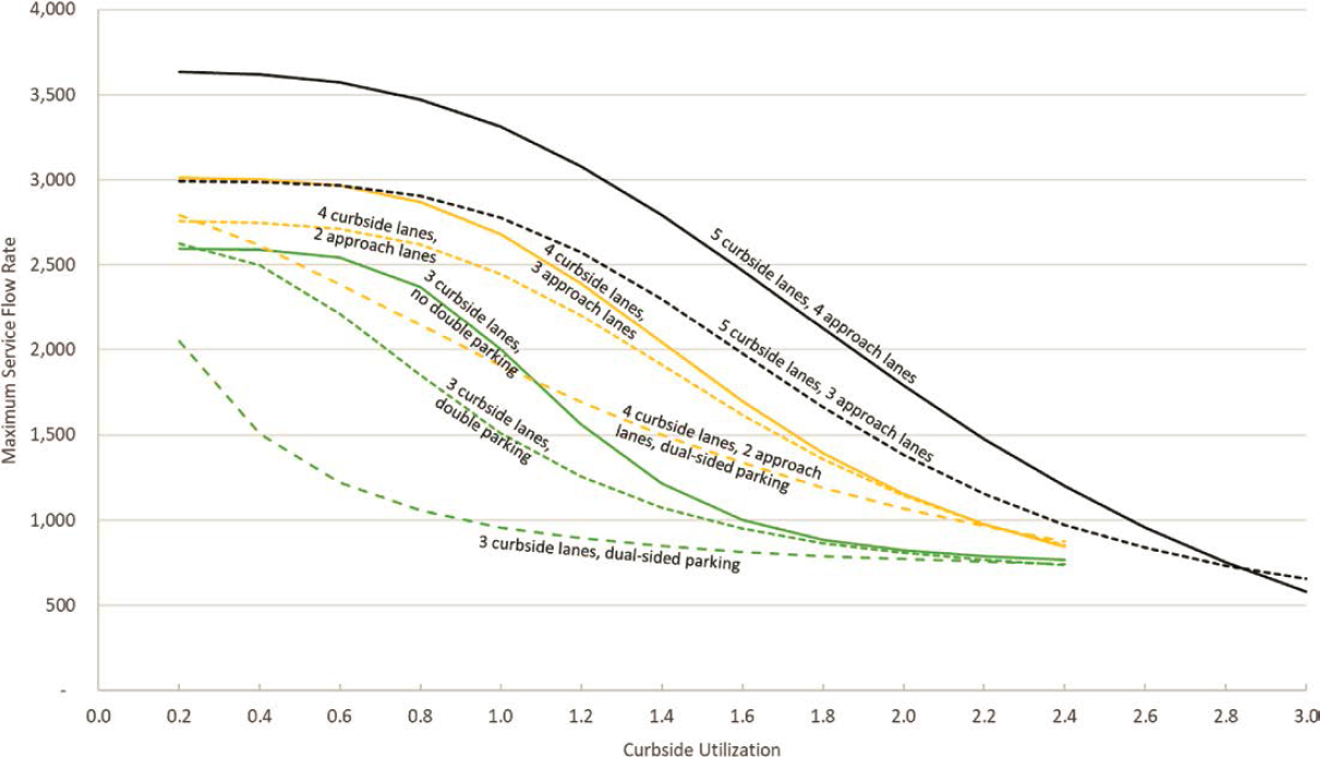
Table C-5. Roadway through capacity model definitions.
| Model | Total curbside lanes | Approach (through) lanes | Parking allowed on both sides? | Double-parking prohibited? | Const A | Const B | Const C | Const D |
|---|---|---|---|---|---|---|---|---|
| 3,2 no dub | 3 | 2 | No | Yes | 736.85 | 0.4672 | 2597.5 | −5.4292 |
| 3,2 dub | 3 | 2 | No | No | 638.72 | 1.291 | 2642.8 | −3.0582 |
| 3,2 dual | 3 | 2 | Yes | No | 650.81 | 5.9473 | 2791.65 | −1.5025 |
| 4,2 | 4 | 2 | No | No | 454.79 | 0.15502 | 2759 | −3.9169 |
| 4,2 dual | 4 | 2 | Yes | No | 117.92 | 0.53449 | 2868 | −1.8199 |
| 4,3 | 4 | 3 | No | No | 472.73 | 0.1506 | 3012.4 | −4.1772 |
| 5,3 | 5 | 3 | No | No | 392.95 | 0.089126 | 2993.2 | −4.184 |
| 5,4 | 5 | 4 | No | No | −373.44 | 0.088833 | 3638 | −3.2659 |
11. Adjusted Through-Lane Roadway Capacity
The lane capacity is multiplied by the Regional Adjustment Factor to obtain the adjusted through-lane capacity, as shown in Equation C-24.
| RdwyThruCapacityAdjustedz = RdwyThruCapacityz * gRegionalAdjFactor | (C-24) |
where
| RdwyThruCapacityAdjustedz = | adjusted capacity for zone z |
| RdwyThruCapacityz = | estimated capacity for zone z |
| gRegionalAdjFactor = | regional adjustment factor |
12. Roadway Volume-to-Capacity Ratio
The roadway volume-to-capacity (v/c) ratio is calculated by dividing the total volume of the study zone by its adjusted through-lane roadway capacity, as shown in Equation C-25.
| (C-25) |
where
| RdwyVCRatioz = | roadway volume-to-capacity ratio for zone z |
| TotRdwyVolz = | flow rate for zone z |
| RdwyThruCapacityAdjustedz = | adjusted capacity for zone z |
Table C-6. Mapping of inputs to through-lane models.
| Driver-side parking | Through lanes | Passenger-side parking | Double-parking prohibited? | Through-lane model | Notes |
|---|---|---|---|---|---|
| 0 | 2 | 1 | Yes | 3,2 no dub | NA |
| 0 | 2 | 1 | No | 3,2 dub | NA |
| 1 | 1 | 1 | No | 3,2 dual | Assumes 2 lane approach. Left approach lane becomes driver’s side parking lane. |
| 0 | 2 | 2 | No | 4,2 | NA |
| 1 | 2 | 1 | No | 4,2 dual | NA |
| 0 | 3 | 1 | No | 4,3 | NA |
| 0 | 3 | 2 | No | 5,3 | NA |
| 0 | 4 | 1 | No | 5,4 | NA |
Note: NA = Not Applicable
13. Roadway Sufficiency
The roadway sufficiency is based on comparing the roadway v/c ratio for each segment to the thresholds given in Table C-7.
14. Crosswalk Capacity with Traffic Signal Control or Traffic Control Officer Control
The methodologies presented in this section are derived from methods in the Highway Capacity Manual (Transportation Research Board 2022). Capacity under traffic signal control is governed by the saturation flow rate for the given lane model and the ratio of effective vehicular green time to the cycle length, using Equation C-26.
| (C-26) |
where
| CCAF = | crosswalk capacity adjustment factor |
| c = | capacity [veh/hr/ln] |
| s = | saturation flow rate [veh/hr/ln] |
| g = | effective vehicular green time [s] |
| C = | cycle length [s] |
In the absence of known signal timing, a default value of CCAF = 0.65 may be assumed.
The effective g/C ratio, or the ratio of effective green time to the cycle length, can be calculated directly if signal timing for the pedestrian crosswalk is known. When traffic control officer control is used, the flagger behavior should be approximated as if it were controlled by a traffic control signal using default values unless field operations are known.
If pedestrian signal timing is known, the effective g/C ratio can be calculated using Equation C-27.
| (C-27) |
where
| W = | walk indication time [s, default = 10 s] |
| L = | length of crosswalk [ft, default = 12 ft/ln] |
| Sp = | pedestrian walking speed [ft/s, default = 3.5 ft/s] |
| C = | cycle length [s, default = 60 s] |
15. Crosswalk Capacity with No Control or Active Warning Devices
It is possible using HCM methods (Transportation Research Board 2022) to estimate the vehicular capacity across a crosswalk with no control or with only active warning devices, such as rectangular rapid flashing beacons. However, the analytical methods to do this require estimates
Table C-7. Roadway sufficiency thresholds.
| Maximum Roadway v/c Ratio, RdwyVCRatioz | Roadway Sufficiency |
|---|---|
| <= 0.60 | Under Capacity |
| > 0.60 to 0.80 | Near Capacity |
| > 0.80 to 1.00 | At Capacity |
| > 1.0 | Over Capacity |
of pedestrian volumes and their likelihood to cross in groups, as well as estimates of driver yielding behavior. Pedestrian volumes and their likelihood to cross in groups are sensitive to activity patterns at the airport and to the specific layout of the airport terminal area that draws pedestrians to cross at a particular location for a specific purpose (e.g., access to parking or courtesy shuttle buses). While estimates of yielding behavior are available for midblock crossings outside of airport environments, little research has been done on the yielding behavior observed within the airport terminal environment. As such, for planning purposes, a default overall crosswalk capacity adjustment factor of CCAF = 0.65 is suggested. If further detail on the pedestrian crossing patterns and driver yielding behavior is known, microsimulation can be used to estimate crosswalk capacity more accurately, as well as determine the effect of the crosswalk on upstream and downstream zones.
References
Highway Capacity Manual 7th Edition: A Guide for Multimodal Mobility Analysis. Transportation Research Board, Washington, DC, 2022.
Hillier, F. S. and G. J. Lieberman. Introduction to Operations Research, 10th ed. McGraw-Hill Education, New York, NY, 2015.
Newell, G. F. Applications of Queueing Theory, 2nd ed. Chapman and Hall, New York, NY, 1982.
Stewart, W. J. Probability, Markov Chains, Queues, and Simulation: the Mathematical Basis of Performance Modeling. Princeton University Press, 2009.
Abbreviations and acronyms used without definitions in TRB publications:
| A4A | Airlines for America |
| AAAE | American Association of Airport Executives |
| AASHO | American Association of State Highway Officials |
| AASHTO | American Association of State Highway and Transportation Officials |
| ACI–NA | Airports Council International–North America |
| ACRP | Airport Cooperative Research Program |
| ADA | Americans with Disabilities Act |
| APTA | American Public Transportation Association |
| ASCE | American Society of Civil Engineers |
| ASME | American Society of Mechanical Engineers |
| ASTM | American Society for Testing and Materials |
| ATA | American Trucking Associations |
| CTAA | Community Transportation Association of America |
| CTBSSP | Commercial Truck and Bus Safety Synthesis Program |
| DHS | Department of Homeland Security |
| DOE | Department of Energy |
| EPA | Environmental Protection Agency |
| FAA | Federal Aviation Administration |
| FAST | Fixing America’s Surface Transportation Act (2015) |
| FHWA | Federal Highway Administration |
| FMCSA | Federal Motor Carrier Safety Administration |
| FRA | Federal Railroad Administration |
| FTA | Federal Transit Administration |
| GHSA | Governors Highway Safety Association |
| HMCRP | Hazardous Materials Cooperative Research Program |
| IEEE | Institute of Electrical and Electronics Engineers |
| ISTEA | Intermodal Surface Transportation Efficiency Act of 1991 |
| ITE | Institute of Transportation Engineers |
| MAP-21 | Moving Ahead for Progress in the 21st Century Act (2012) |
| NASA | National Aeronautics and Space Administration |
| NASAO | National Association of State Aviation Officials |
| NCFRP | National Cooperative Freight Research Program |
| NCHRP | National Cooperative Highway Research Program |
| NHTSA | National Highway Traffic Safety Administration |
| NTSB | National Transportation Safety Board |
| PHMSA | Pipeline and Hazardous Materials Safety Administration |
| RITA | Research and Innovative Technology Administration |
| SAE | Society of Automotive Engineers |
| SAFETEA-LU | Safe, Accountable, Flexible, Efficient Transportation Equity Act: A Legacy for Users (2005) |
| TCRP | Transit Cooperative Research Program |
| TEA-21 | Transportation Equity Act for the 21st Century (1998) |
| TRB | Transportation Research Board |
| TSA | Transportation Security Administration |
| U.S. DOT | United States Department of Transportation |


