Evaluating the Performance of Longitudinal Barriers on Curved, Superelevated Off-Ramps (2025)
Chapter: 3 Vehicle Dynamics Analyses
CHAPTER 3
Vehicle Dynamics Analyses
Vehicle dynamics analysis (VDA) was used in previous efforts to analyze barrier effectiveness for CSRSs to assess the trajectories of vehicles leaving the traveled way. This approach proved to be highly effective in understanding the interfaces of errant vehicles with various types of barriers in previous research on CSRSs. Therefore, the same VDA tools were used to develop an improved understanding of the effectiveness of longitudinal barriers used on CSORs. A vehicle departing the driving lanes on a CSOR is influenced by the same factors, including ramp curvatures, superelevation, vertical grade, shoulder and roadside designs, and barrier features. Given that such departures can occur on CSOR ramps of varying configurations, a similar VDA approach was considered appropriate. This VDA needed to reflect the features that would influence the dynamic response of vehicles leaving on-ramps. The roadway, shoulder, and barrier applications for these situations were defined.
Vehicle dynamics simulations were used in the initial phase of the study to yield quick analysis and understanding of the trajectories of errant vehicles on curved, superelevated ramp sections. The insights from these analyses were used to determine the most critical finite element crash simulations needed to investigate in much greater detail. VDA can simulate the trajectory of vehicles in three dimensions, considering the design features of the vehicle (e.g., wheelbase, weight or mass, suspension characteristics), the operating conditions (e.g., speed, driver inputs), and the influence of the surface terrain over which the vehicle is traveling (e.g., slope, grade, friction, softness). VDA uses concepts of free-body physics for the movement of a sprung mass for specific velocity, accelerations and decelerations, and surface conditions to determine vehicle trajectories, including roll, pitch, and yaw factors, for small increments of time.
Two vehicle dynamics software programs were used in this study to predict the vehicle trajectories on curved, superelevated ramps: HVE (Human, Vehicle, and Environment, by the Engineering Dynamics Company) (23) and CarSim (by Mechanical Simulation Corporation) (24). The programs were developed for use by engineers and safety researchers to study interactions among humans, vehicles, and their environment. HVE and CarSim are high-level simulation tools aimed at creating three-dimensional models of vehicles and environments, allowing the study of their dynamic interaction under selected conditions. The tools provide a detailed description of a motor vehicle’s trajectory, considering the influence of weight, suspension system, and other vehicle factors. Available databases include a wide range of high-fidelity vehicle models that can be used in dynamic reconstructions and simulations.
HVE and CarSim provide physical and visual environment models to simulate selected conditions. Weather attributes, road geometry, and pavement-friction properties can be computed and their effects on vehicle dynamics analyzed. Drivers’ actions (e.g., throttle, brakes, steering, gear selection) can also be simulated. The models have been thoroughly validated and are capable of accurately predicting a vehicle’s trajectory for different terrain profiles. The research team used
these programs in previous research studies to assess vehicle-to-barrier interaction when the barrier is placed on non-level terrain (25–29).
3.1 Vehicle Dynamics Analyses
Undertaking VDA required physical information about the vehicles and the barriers to be studied, as well as data on ramp configurations (e.g., grade superelevation, side slope), barrier design features, effective interface areas, and the terrain or surface conditions associated with CSORs. The factors considered in the VDA were:
- Vehicle types
- 1100C small car (Toyota Yaris)
- 2270P pickup truck (Chevrolet Silverado)
- Barrier types
- W-beam guardrail (27.75-in. and 31-in. top-of-rail height)
- Thrie beam guardrail (34-in. top-of-rail height)
- Concrete barriers (32-in. and 42-in. top height)
- Superelevation and curvature
- 4%, 6%, and 8% ramp cross slope
- 150-ft, 300-ft, and 450-ft curvature radius
- Impact conditions
- Impact angle: 5, 10, 15, 20, and 25 degrees
- Impact speed: 50, 70, and 100 km/h (31, 43.5, and 62 mph)
- Shoulder width and slope
- 4-ft, 8-ft, and 12-ft widths
- 0%, 3%, 6%, and 8% (angle relative to road)
- Other variations
- Ramp grade: 0%, −4%, and −8% (downward)
The following sections describe the VDA setups, the factors considered, the use of software, and the cases selected for analyses.
3.1.1 Vehicle-to-Barrier Interface Considerations
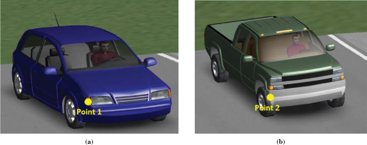
The study focused primarily on two types of vehicles commonly used for roadside hardware testing: a 1100C small car (1,100 kg) and a 2270P pickup truck (2,270 kg). The specific weight, size, frontal geometry, and suspension systems of these vehicles were incorporated into the VDA model such that they would match typical MASH test vehicles (namely a Toyota Yaris sedan and a Chevrolet Silverado pickup truck).
In these analyses, one point was defined for each type of vehicle and considered to represent its primary interface (engagement) region. These points are labeled 1 and 2 in Figure 6. The primary interfaces are located at positions on the front of the vehicles that are believed to represent the engagement point that differentiates between tendencies to override or underride a barrier. Point 1 for the small vehicle is located at a height of 21 in., while Point 2 for the pickup has a height of 25 in. These point positions were defined by examining the frontal profile of each vehicle and reviewing full-scale crash tests conducted using similar vehicles. The traces of these points are critical in determining the interface with barriers for any vehicle trajectory.
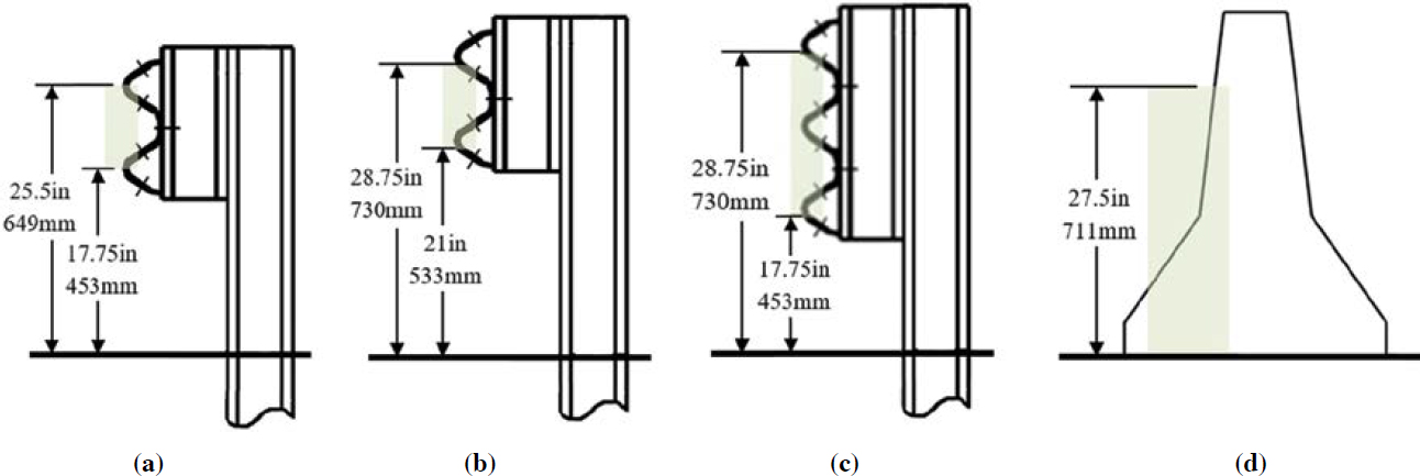
Various barriers were selected for analysis, and an interface region was defined such that if the critical points (Point 1 or Point 2) are inside this region at the start of the impact, the barrier is considered likely to redirect the vehicle. If Point 1 (from the small car) falls below the interface
region, an underride or significant snagging is likely to occur. Similarly, if Point 2 (from the pickup truck) is above the interface region, vehicle override is likely to occur. The interface regions for some of the barriers analyzed are shown in Figure 7. For each of the barriers, the interface region is represented by a green-shaded box with the corresponding maximum and minimum heights. These regions are based on the geometry of the barrier and a review of full-scale crash tests conducted on these barriers. For concrete barriers, only the override condition is considered; therefore, there is no minimum height.
Interface analyses accounted for the effects of vehicle orientation (changes in roll, pitch, and yaw angles) in computations to determine the positions of Points 1 and 2 relative to the vehicle’s center of gravity. Further, variations in the designs of the barriers, such as the inclusion of rub rails, increased heights, or different shapes for the concrete barrier, were not considered. The evaluations based on these interface regions were used in the VDA only as preliminary criteria to identify cases to be simulated in the finite element analysis. The actual impact is simulated in the finite element evaluations and the barrier performance is assessed on the basis of these results.
3.1.2 Ramp Curvature and Grading Conditions
Using information collected from the state agency survey, this study considered various degrees of ramp curvature to reflect the range of applications commonly found on highways.
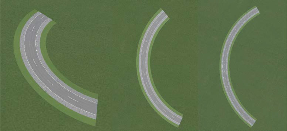
A total of nine roadway curve conditions with different superelevations (4%, 6%, and 8%) and curvatures (150, 300, and 450 ft) were analyzed in the VDA to investigate crash simulations. Figure 8 describes the types of ramp curvature considered in the VDA and crash simulations.
3.1.3 Analysis of CSOR Vehicle Trajectories
Figure 9 illustrates the typical path or trajectory (via sequential vehicle images) of a vehicle negotiating a curve before departing the ramp, as marked by the red line. The cross section of a superelevated curve perpendicular to the centerline (indicated by the black line) is depicted. The banking of the roadway surface is exaggerated in this case. The shoulders can be designed to have the same slope relative to the roadway cross section or to have negative slopes for drainage. The red line shows the typical path or horizontal trajectory of an errant vehicle leaving the road on a CSOR. The figure shows a rising surface, reflecting a diagonal crossing of the superelevation followed by a diagonal traversing of the negative shoulder and side slope.
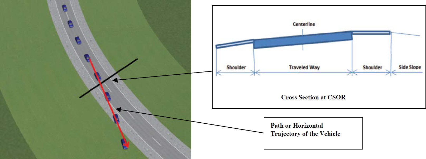
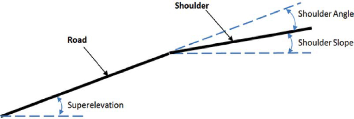
Table 3. Shoulder slopes used in VDA.
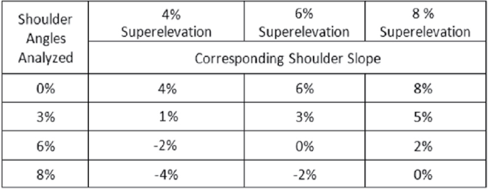
In the VDA, the vehicle was run a distance of about 330 ft (100 m) on this surface to be in a “curve operation” equilibrium state before it was directed off the road. Several defined departure paths were input into the software to represent various departure angles. Repeated simulations of vehicles traversing such paths were conducted, varied to reflect exit angles of 5, 10, 15, 20, and 25 degrees for vehicles traveling at 31, 43.5, and 62 mph (50, 70, and 100 km/h). The roadway-to-shoulder angles analyzed are depicted in Figure 10 with a 12H:1V roadside slope. Table 3 lists the shoulder angles (defined as the angle relative to the road and different from the common shoulder slope definition) relative to the road that were used and the corresponding shoulder slopes.
3.2 Vehicle Dynamics Analyses Results
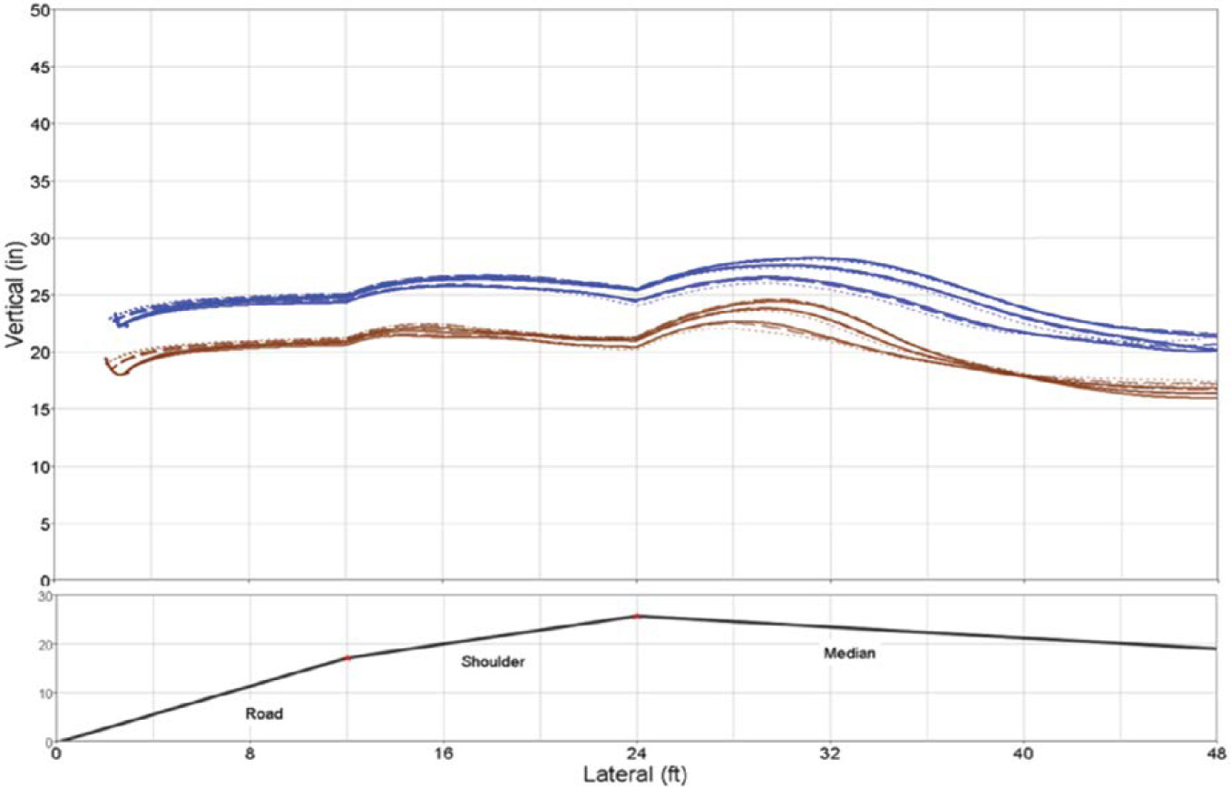
The VDA software was used to generate trajectories for each vehicle at the selected exit angles and speeds for each road departure condition. Figure 11 shows the vertical trajectories or trace paths of Point 1 for the 1100C vehicle (brown) and Point 2 for the 2270P vehicle (blue) negotiating a curve and departing onto the roadside at different speeds and angles. Multiple curves reflect variations in departure speed and angle for each vehicle, speed, and angle. The differences in basic vehicle heights are reflected by the relative positions of the two sets of curves. Consistency is present in the heights with the road profile shown by the black line at the base of the graph. Dynamic effects of the sprung mass cause the curves to vary for the changes in cross-section conditions. A similar graph was generated for each set of conditions in the analysis matrix.
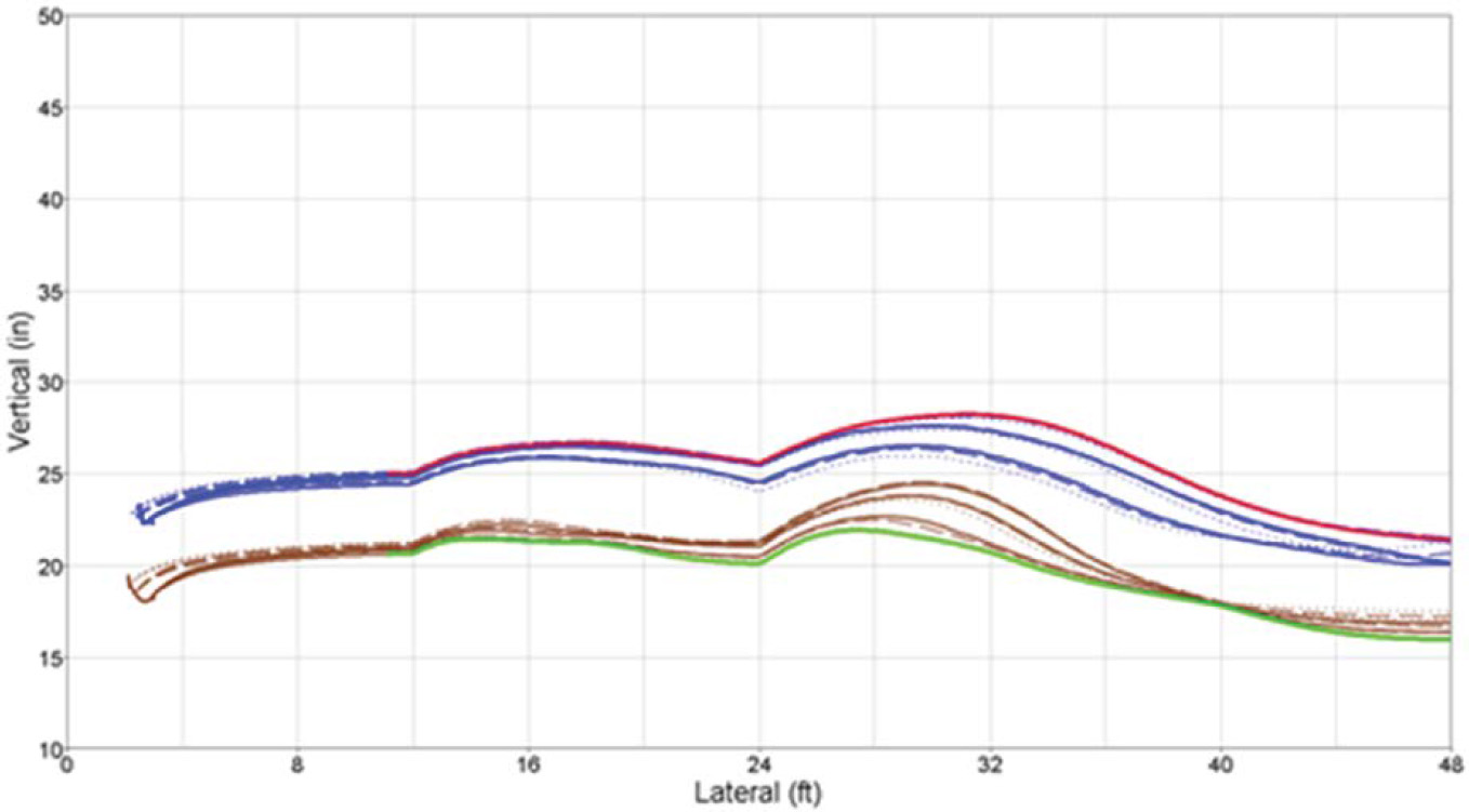
Figure 12 provides an example of the normalized representation of the vertical trajectory for the same conditions. In the normalized view, the variations in trajectory are indicated relative to a horizontal plane as opposed to the actual cross-section surface. The curve on the bottom shows

the road profile or cross section as a reference for the vehicle dynamics traces. The normalized view provides a convenient means to analyze and compare vehicle dynamics effects for different conditions simultaneously. The normalized version is also useful for translating the vertical trajectories to a common plane to allow the aggregation of groups of results to define limits.
Figure 13 illustrates a primary use of the normalized graphs of the trajectory data. All trajectory traces for a given set of CSOR conditions were plotted to derive maximum and minimum limit curves. The bold red line represents the maximum trajectory height limit across the entire path, while the bold green line indicates the minimum trajectory height. These limits indicate the requirements for any barrier system in that roadside configuration for all lateral positions beyond the shoulder. This approach can be used to determine the potential effectiveness of varying barrier systems across all possible lateral positions for a given roadside configuration.
Figure 14 shows more specific examples of how the plot of maximums and minimums can be applied. For a given superelevated curve and roadside configuration (e.g., 150-ft radius curvature, 6% superelevation, 8-ft shoulder width, 6% shoulder angle, and −6% vertical grade), the limits can be plotted along with the interface area provided by a specific barrier. These interface areas are represented by the blue and green lines that reflect the maximum and minimum vertical positions of the vehicle’s critical points as it leaves the roadway and moves onto the roadside. For the barrier to be effective, it must have a good interface for both large and small vehicles at any given lateral position. The graph shows the limits for the 31-in. W-beam MGS (or Midwest Guardrail System) barrier as yellow lines across the graph for various positions where the barrier can be placed. If the maximum and minimum limits fall within the yellow lines, then the barrier will have a good interface for both types of vehicles. Where the blue line goes above the top yellow line, the possibility of an override exists. Where the green line falls below the lowest yellow line, the possibility of an underride exists.
The lower portion of Figure 14 shows the profile or cross section of the road related to the upper graph. Effective placement areas are shown in this pane. The red-shaded area defines the lateral

positions where the specific barrier has an interface area above the maximum lower height limit (green curve), below the minimum height limit (blue curve), or both. Effective lateral placement occurs where both criteria are met, and this is shown shaded green. Plots of this type for all selected curve and roadside configurations were generated and are presented in Appendix C. Because of the large number of configurations considered in the study, plots from only one of the barriers analyzed (the 31-in. top-of-rail height W-beam barrier) are included in Appendix D and Appendix E. Similar plots were generated for the other barriers and can be supplied upon request.
3.3 Aggregated VDA Metrics for CSORs
The VDA simulations were used to determine the maximum and minimum heights of the critical points on the bumper (Points 1 and 2) as the vehicle first comes in contact with the barrier. Barrier lateral placement in these evaluations was 1 ft off the shoulder for each of the three barrier systems selected. All combinations of curvature, superelevation, and shoulder width and slope for the different speeds and impact angles were used in the evaluations. The maximum and minimum heights are shown in Table 4 to Table 9. These tables show the critical heights for the four analyzed barriers with all speeds (31, 43.5, and 62 mph) and angles (5, 10, 15, 20, 25 degrees) considered. Table 8 and Table 9 show the results for the 27.55-in. and 31-in. top-of-rail height W-beam barriers with only the lower speed (31 mph) considered. Each cell represents the barrier height for the specific conditions. If the value is shaded red, it implies that the height is outside the limits (i.e., too high or too low) and hence indicates that there is not a “good” interface. These tables, as well as the other interface plots, are used to provide the basis for determining those cases or types of cases that need to be analyzed with crash finite element simulation.
Table 4. Vehicle interfaces for 27.75-in. W-beam [G4(1S)] system for all speeds and angles.
![Vehicle interfaces for 27.75-in. W-beam [G4(1S)] system for all speeds and angles](https://www.nationalacademies.org/index.php/read/28589/assets/images/tab-4.jpg)
Table 5. Vehicle interfaces for 31-in. W-beam (MGS) system for all speeds and angles.

Table 6. Vehicle interfaces for Thrie beam (SGR09b) system for all speeds and angles.

Table 7. Vehicle interfaces for 32-in. concrete barrier for all speeds and angles.
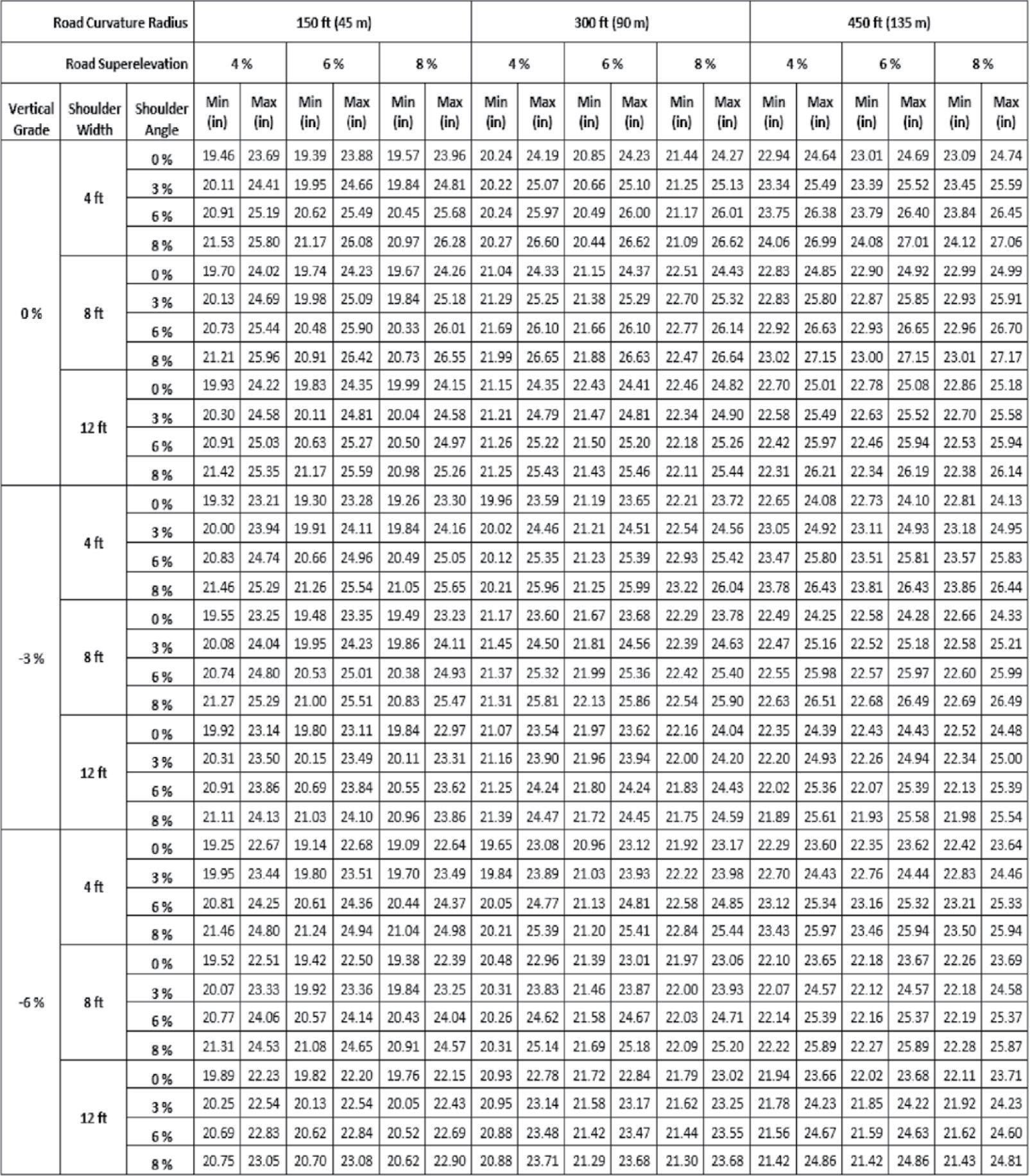
Table 8. Vehicle interfaces for 27.75-in. W-beam [G4(1S)] system for low speeds (31 mph).
![Vehicle interfaces for 27.75-in. W-beam [G4(1S)] system for low speeds (31 mph)](https://www.nationalacademies.org/index.php/read/28589/assets/images/tab-8.jpg)
Table 9. Vehicle interfaces for 31-in. W-beam (MGS) system for low speeds (31 mph).

Looking across all the values in the table, it can be seen that the critical heights range from just under 21 in. to almost 28 in. When examining the results in each of the tables, some of the following insights can be noted:
- For the 32-in. height concrete barriers:
- Because the concrete barrier has a 0-in. minimum interface height (i.e., no potential for underrides), this barrier works for all minimum cases for all the curvature, superelevation, shoulder, and vertical grade conditions. It can be observed from Table 7 that no red values are in any of the minimum rows.
- Similarly, this barrier provides a good interface for all offsets by noting no red values.
- Because the VDA showed good vehicle-to-barrier interface for the 32-in. height concrete barriers, it can be concluded that the 42-in. height barriers would also have adequate interface. (Finite element analyses would be needed to assess the effects of impact severity.)
- For the Thrie beam barrier (SGR09b):
- VDA indicates that the Thrie beam barrier meets the minimum interface requirements for all cases (Table 6), indicating less susceptibility to underride for the CSOR road profiles and impact conditions considered.
- Similarly, the greater height of the Thrie beam barrier led to all “good” maximum interface indications across the range of conditions considered, indicating less susceptibility to override for the CSOR road profile.
- For the W-beam barrier with 27.75-in. top-of-rail height (G4(1S)):
- The G4(1S) barrier appears to meet the minimum interface requirements for all cases, as Table 4 shows no red-shaded cells for any of the minimum columns, indicating less susceptibility to underride for the CSOR road profiles and impact configurations considered.
- Table 4, however, shows cases in which the maximum requirement is not met, as indicated by the red-shaded cells. Hence, there is an increased chance of override from the CSOR road profile. Red values are more noticeable with the higher shoulder slope angle (8%), lower vertical grade (0%), and higher curvature (450 ft).
- In Table 8, only the lower speed (31 mph) is considered, as fewer cases of override were observed.
- For the W-beam barrier with 31-in. top-of-rail height (MGS):
- The greater height of the MGS barrier provides more adequate maximum interface indications across a range of conditions, indicating less susceptibility to override with the CSOR road profile compared with the G4(1S) system (Table 5).
- However, there is no corresponding meeting of the minimum requirements. Several cells in Table 5 do not meet this criterion, indicating susceptibility to a vehicle going under the barrier and its potential for snagging posts. Cases are more noticeable for sharper CSORs (150 ft).
- Much fewer cases of underride were observed when considering only the lower-speed (31 mph) cases, as seen in Table 9.
These and other insights demonstrate the value of the VDA results. VDA provides an indication of how well or poorly the barrier would perform based on the vehicle dynamics and geometry of the barrier. It does not account for the increased or decreased severity of the impact attributable to changes in vehicle orientation and speed. This aspect of performance is analyzed using finite element simulations and crash testing in the next chapter.


