Thriving on Our Changing Planet: A Decadal Strategy for Earth Observation from Space (2018)
Chapter: 3 A Prioritized Program for Science, Applications, and Observations
3
A Prioritized Program for Science, Applications, and Observations
The committee was charged with developing a prioritized list of top-level science and application objectives to guide space-based Earth observations over the next 10 years, and identifying gaps and opportunities in the Programs of Record (PORs) at the National Aeronautics and Space Administration (NASA), National Oceanic and Atmospheric Administration (NOAA), and U.S. Geological Survey (USGS) in pursuit of those top-level science and application challenges. This chapter describes the process used by the committee to identify and prioritize observational needs, and defines a robust and balanced U.S. program of Earth observations from space consistent with agency-provided budget expectations. The resulting program, built on the foundation of the U.S. and international PORs, addresses exciting and societally relevant questions and challenges in Earth system science while providing the programmatic flexibility needed to leverage innovation and opportunities that occur on subdecadal time scales.
THE ESAS 2017 PRIORITIZATION PROCESS
Community Input
Prior to the start of the decadal survey, the standing Committee on Earth Science and Applications from Space (CESAS) issued the first request for information (RFI-1) to the community, soliciting white paper submissions describing key challenges in Earth system science. In addition to providing important input into the identification of major challenges that can be substantially advanced through space-based observations, the responses informed the structure of the panels that were established by the steering committee. A second RFI (RFI-2), issued by the steering committee, called for submittal of “specific science and applications targets (i.e., objectives) that promise to substantially advance understanding in one or more Earth system science themes.” Approximately 300 white papers were submitted in response to the two calls, spanning all areas of Earth science.
Approach and Process
The 2017 decadal survey was led by a steering committee and supported by five interdisciplinary panels. Steering committee members were selected to represent the broad Earth system science and applications community.
Process
The steering committee, in close collaboration with the panels, developed and implemented a process for establishing Science and Application Priorities and determining the resulting Observing System Priorities required to address them. The steps that were used to converge from a large set of possibilities to a final, small set of priorities, and the roles of the community, committee, and panels are shown using the analogy of a narrowing pyramid in Figure 3.1 and are discussed further later. From the hundreds of suggestions
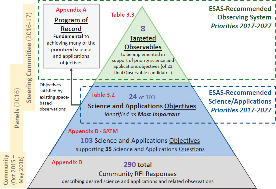
for science and applications priorities submitted through the RFI process and/or considered by the panels, only a much smaller number (103) were considered as formal priorities, and only a small portion of those (24) were ranked among the highest priorities.
Addressing the Statement of Task
As summarized in this report’s preface, the committee’s statement of task (SOT) requested that priorities focus on science, applications, and observations, rather than the instruments and missions required to carry out those observations. The SOT described a multistep requirements development process, diagramed in Figure 3.2, leading from science to observations through a step referred to in the SOT as “science

targets.”1 A science target, as defined in the SOT, is “a set of science objectives” related by a common space-based observable. The committee defined the observable associated with each science target as a Targeted Observable.
In accordance with the SOT, and with the goal of simplifying the presentation of its priorities, the committee chose to focus on two key elements of this sequence for prioritization: (1) the science and applications objectives (blue, corresponding to Table 3.2 on p. 81) and (2) the Targeted Observables (green, corresponding to Table 3.3, on page 118). Example measurements and missions were identified and evaluated only for the purpose of ensuring cost and technical readiness feasibility for Targeted Observables recommended within the NASA program, as required by the SOT.
Panels
Informed by the first RFI submission, the steering committee constructed a set of five interdisciplinary panels to facilitate community engagement in the decadal survey. Panel members were drawn from the scientific community based on their disciplinary and interdisciplinary expertise. The panels, each consisting of approximately 15 members, met three times, with the first and last of these meetings being conducted in a “jamboree” format in which all of the panels met in parallel at the same venue to identify and discuss where their science and application priorities intersected. The first panel jamboree also coincided with a meeting of the full steering committee and included joint plenary sessions to identify and discuss science priorities and areas where priorities might intersect. The second jamboree, and each of the stand-alone panel meetings, included participation by steering committee member representatives who helped facilitate communications between the steering committee and panels throughout the study. The five panels are listed here:
- Global Hydrological Cycles and Water Resources. The movement, distribution, and availability of water and how these are changing over time.
- Weather and Air Quality: Minutes to Subseasonal. Atmospheric dynamics, thermodynamics, chemistry, and their interactions at land and ocean interfaces.
- Marine and Terrestrial Ecosystems and Natural Resource Management. Biogeochemical cycles, ecosystem functioning, biodiversity, and factors that influence health and ecosystem services.
- Climate Variability and Change: Seasonal to Centennial. Forcings and feedbacks of the ocean, atmosphere, land, and cryosphere within the coupled climate system.
- Earth Surface and Interior: Dynamics and Hazards. Core, mantle, lithosphere, and surface processes, system interactions, and the hazards they generate.
The panel order in this list was chosen by the committee to simplify the presentation of the material and not to reflect any prioritization of the panels. This ordering is maintained throughout the discussion in this section and in various tables throughout the report. The panels developed science and applications priorities for their panel topic areas, based in large part on the input received through the RFI responses, and further informed by the expertise of the panel members and steering committee liaisons. Panel RFIs
___________________
1 Interpreted by the committee more broadly to be science and applications targets, in keeping with the nature of the report.
are not cited directly in this report, since the intent was to use them as guidance and not to suggest preference for particular RFIs within the report’s priorities. The panels were directed to interpret their scope broadly, considering the state of science in both their encompassed traditional disciplines as well as with a broader view of Earth system science. Reports of each panel are included as chapters in Part II of this report; see Box 3.1 for further information.
Integrating Themes
The steering committee identified a set of Integrating Themes to complement the panel deliberation process by ensuring explicit consideration of broad, thematic concepts that cut across multiple panel domains. Members of the steering committee and representatives of each panel participated in an Integrating Themes Workshop during which priorities were considered in the context of advancing key aspects of Earth system science (e.g., the Carbon Cycle, the Water and Energy Cycles, Extreme Events) outside the traditional panel structure. While no separate report has been prepared from this workshop, the broad thinking of the workshop is reflected in the analysis of observation priorities and the development of the committee’s recommendations.
The Integrating Themes developed at this workshop were used early in the decadal survey process to ensure important Earth system priorities were not missed by discipline-focused panels. Later, the steering committee leveraged this Integrating Themes perspective to ensure the recommended program addressed key system priorities. These themes, and their implications for the committee’s priorities, are discussed throughout this chapter.
Budget Assumptions and Cost Assessment
Translating the committee’s science and applications priorities into an observing program required that the committee assess the likely cost of the proposed observations to ensure the program can be accomplished within a budget consistent with agency expectations.2
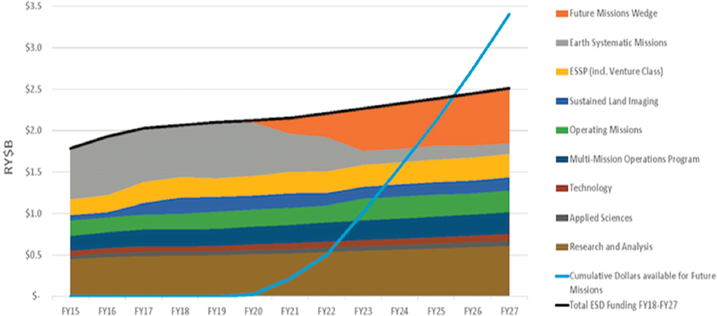
In accordance with sponsor input to the decadal survey, the committee adopted a baseline NASA budget scenario that assumes that the budget provided in the Earth Science Division (ESD) POR will grow only at the rate of inflation, as shown in the “sand chart” in Figure 3.3. The cost of the flight missions in the POR (ICESat-2, NISAR, PACE, SWOT, Sentinel-6, GRACE-FO, RBI, TSIS-1/2 and CLARREO PF) from the start of fiscal year (FY) 2018 through the end of FY 2027 results in a lien of $3.6 billion from the prior decadal interval.3 This baseline budget then implies a total of $3.4 billion available to invest in the coming decadal survey’s priorities (FY 2018 through FY 2027), beyond funds already allocated and assuming existing program elements remain unchanged. This value corresponds to the orange portion of Figure 3.3. It is noteworthy that in this scenario, funding for implementing this decadal survey’s flight priorities does
___________________
2 The statement of task says, “The survey committee will work with NASA, NOAA, and USGS to understand agency expectations of future budget allocations and design its recommendations based on budget scenarios relative to those expectations.” NASA Earth Science Division (ESD) provided a budget history to the committee and indicated that large-scale changes to recent funding levels were not anticipated. The committee thus based its recommendations on the assumption that the current budget would grow with inflation. Decision rules are established in Chapter 4 to describe how the program can be tailored to accommodate modest budget shortfalls and how it can best be expanded to take advantage of any additional resources that may become available throughout the decade.
3 See discussion in Chapter 3 of NRC (2015b, pp. 57-58).
not emerge until approximately FY 2020, as the flight program’s resources are fully consumed with the POR until that time.
The committee notes that its recommendations are provided with a series of decision rules (see Chapter 4), which allow NASA to readily respond with program augmentations consistent with decadal survey priorities to take advantage of any additional funds that may be made available to support Earth system science throughout the decade. Similarly, these decision rules provide guidance on how to implement program reductions in the face of reduced resource availability.
Responsive to the study’s statement of task, the committee used an independent Cost Assessment and Technical Evaluation (CATE) process to ensure concepts were credible and costs were of comparable fidelity when cost was a factor in prioritization. Drawing from the NRC The Space Science Decadal Surveys: Lessons Learned and Best Practices report (NRC, 2015b), the committee first used a cost “binning” approach to determine the relative scale of investment (i.e., small, medium, large) required for each potential program augmentation prior to down-selecting which program elements required more detailed cost estimation. Full CATE studies were completed by The Aerospace Corporation for explicitly prioritized program elements, which were binned as large (>$500 million).
Program of Record
The existing U.S. and international POR, which is summarized in Appendix A, forms the foundation upon which the committee’s recommendations are established. The POR includes NASA, NOAA, and USGS missions formally planned and budgeted per input from these agencies, and those partner missions for which either NASA or NOAA explicitly expressed a commitment to this committee. This appendix also lists anticipated additional space-based observation contributions from other space agencies, but the commitments to these programs were not verified by the committee (these nonverified programs have the additional challenge that even when commitments are real, data may not be reliably available to NASA and NOAA researchers). Some items in this list (e.g., QuikSCAT) are known to currently have degraded performance, which was taken into account by the committee in its deliberations.
To identify gaps in the POR, the steering committee members and panel representatives attended a workshop during which the measurement needs to address priority science and applications objectives in the next decade as identified in the Science and Applications Traceability Matricies (SATMs) were reviewed against the POR to determine whether existing or planned measurements were adequate to meet the stated objectives. Where the POR did not adequately meet the need to address a high-priority objective, participants identified candidate augmentations to the POR to address the unmet need. Observations not in the POR were aggregated, as summarized in Appendix C, and became the starting point for the committee’s deliberations regarding needed unmet observations.
The POR, and reliable funding to ensure its implementation, are particularly important. Earth system science and applications rely on long-term sustained observations of many key components of the Earth system. The POR provides many of the coming decade’s needed continuity measurements, with a significant portion of that investment coming from internationally coordinated networks of operational satellites. Two such networks are the meteorological satellites coordinated by the Coordination Group for Meteorological Satellites (CGMS) and the more recent Sentinel satellites of the European Union’s Copernicus Program (see Box 3.2), which together will provide continuity for a broad range of critical Earth observations.
The Sentinels will reach full operational status in 2023 and will sustain this observational capability for at least a decade. Given that the United States has no equivalent capability to this operational Earth observation and monitoring program in Europe, the committee recognizes the importance of Copernicus in general and the Sentinels in particular as a long-term, continuing source of a variety of important observations. It is clearly in the interest of the U.S. agencies and the research community for the U.S. agencies to
ensure that their investigators have access to Sentinel observations in a timely manner. If the United States cannot replicate an effort like Copernicus and the Sentinels, U.S. agencies would benefit substantially from exploring options for complementing and strengthening this European effort, such as is being done by NASA and NOAA with the JASON-CS satellite partnership for Sentinel-6.
Science and Applications Traceability Matrix
Achieving traceability of both science/applications and observing system priorities was central to the committee’s work. The foundation for this traceability was the SATM developed by the steering committee in conjunction with the panels, with content provided primarily by the panels. It establishes the traceability from prioritized science/applications to needed observing systems. The complete SATM is included in Appendix B. A shorter summary of the science and applications priorities within the SATM is provided as Table 3.2, below; this table provides the basis for the ESAS 2017 prioritized science and applications.
Development of the SATM was accomplished in four steps, as shown in Figure 3.2: (1) establish the priority science/applications question or goals; (2) identify a set of objectives (quantified when possible) needed to pursue those questions/goals; (3) determine the observables needed to fulfill those objectives; and (4) characterize the measurements available to make the observations.
The development of the SATM began with the committee issuing a second community RFI-2 soliciting specific science and applications needs (i.e., specific measurements/observations, or theory and/or modeling activities) that promise to advance existing or new scientific or applications objectives, contribute to fundamental understanding of Earth system science, and/or facilitate the connection between science and societal benefits (see Figure 3.1 and accompanying caption). The RFI responses provided a basis for panel deliberations, with each panel considering relevant RFI responses as it developed a set of key science and applications goals for the decade ahead. Panels then developed their SATM contributions to capture decadal goals and develop them into quantifiable objectives that might be addressed by space-based observations.
The prioritization of the Earth science/applications objectives within the SATM was accomplished using three categories:
MI—Most Important. Refers to objectives that are critical in order to make substantive advances in knowledge in key areas identified by the panel. These are the highest-priority objectives that should be pursued even under the most minimal of budget scenarios.
VI—Very Important. Refers to objectives that would contribute substantially to advances in knowledge in key areas identified by the panel and should be supported, second only to MI. Every effort should be made to accomplish these if resources are available or if they can be done opportunistically as a cost-effective add-on to an existing mission.
I—Important Refers to objectives of high value that should be addressed if resources allow or if cost-effective opportunities are found to address them.
Observations often satisfy multiple objectives; therefore, some observations that are targeted at addressing MI priorities will also address VI and I priorities as well. A prioritized observing program, focused on achieving MI science and applications priorities, would be expected to achieve some (or even many) VI and I priorities at no additional cost.
Methodology for Establishing SATM Importance Ranking
The importance values ascribed to each science and applications objective within the SATM were based on the expert judgment of each panel, informed by the RFI submissions and available peer-reviewed literature. The allocation of importance into three categories was carried out by the panels and was accomplished through an iterative process by which the importance of each science and application objective was established using a score that was normalized both within and across panels. Based on these scores, the objectives were then binned into the categories of Most Important, Very Important, and Important. Because of the many possible considerations that can influence the assessment of scientific and applications importance, a rigid framework of specific considerations was not used. However, panels were encouraged to review the considerations listed in Table 3.1 to guide their discussions. Each panel, and the individual members of that panel, was free to choose its own considerations. The steering committee monitored the ranking process and concurred with the results.
During its deliberations, the committee noted that each SATM question generally involved aspects of both curiosity-driven and applications-driven science, which thus led to observations that addressed both exploratory and continuity-related needs. The fact that such basic and applied science categories have largely merged over the last decade is a tribute to a community success: restructuring our field in an integrated Earth context that balances science with applications and combines exploratory and continuity-related observations.
In developing this ranking approach, the committee reviewed the quantitative methodology described in the report Continuity of NASA Earth Observations from Space: A Value Framework (NRC, 2015a). While the merits of a fully quantitative valuation as recommended in the Continuity Report were attractive, the practical aspects of completing such valuation over a hundred objectives, as needed for this ESAS 2017 report, precluded that approach. It would have required reliable quantitative evaluation of five factors for these objectives, meaning thousands of quantitative assessments—each of which requires documented justification. Furthermore, the committee recognized that the factors relevant for the specific task of making continuity decisions may not be sufficient for the broader task of identifying observing system priorities.
TABLE 3.1 Considerations for the Importance Factor Used to Evaluate Science/Applications Objectives Within the SATM as Presented in Appendix B (Not in Priority Order)
| Area | Description |
|---|---|
| Science Questions | Science objectives that contribute to answering the most important basic and applied scientific questions in Earth system science. These questions may span the entire space of scientific inquiry, from discovery to closing gaps in knowledge to monitoring change. |
| Applications and Policy | Science objectives contributing directly to addressing societal benefits achievable through use of Earth system science. |
| Interdisciplinary Uses | Science objectives with benefit to multiple scientific disciplines, thematic areas, or applications. |
| Long-Term Science and/or | Objectives that can support scientific questions and societal needs that may arise in the future, even if |
| Applications | they are not known or recognized today. |
| Value to Related Objectives | Science objectives that complement other objectives, either enhancing them or providing needed redundancy. |
| Readiness | Are we in a position to make meaningful progress to advance the objective, regardless of measurement? |
| Timeliness | Is now the time to invest in pursuing this objective? Examples include recently occurring phenomena that require focused near-term attention and the existence of complementary observing assets that may not be available in the future. |
As a result, the committee chose to embrace the general guidance of the Continuity Report regarding a traceable (though not fully quantitative) prioritization process. Traceability is documented, to the extent possible, through the structure of the SATM (Appendix B), as discussed earlier. A prioritized assessment of the SATM’s science/applications objectives was achieved through evaluating the Importance factor in the SATM, using a rigorously normalized process guided by judgment of the committee and panels.
The SATM Importance ranking (the rightmost column in Table 3.2) thus represents the committee’s assessment of the pure science and applications priorities (consistent with the input provided by the panels), independent of implementation considerations such as cost. The inclusion of cost, feasibility, and readiness constraints was accomplished subsequently, when the science and applications priorities were translated into needed observations (to be ultimately implemented as instruments or missions), as discussed in the following sections. This resulted in some situations where highly ranked science and applications are not reflected in the committee’s observing system recommendations when the observations proved too costly or appeared not ready for implementation. In such cases the high science and applications ranking suggests that investment in maturing the science or technology could have a substantial payoff.
The steering committee interacted directly with the panels during the development of priorities, which underwent a final review to ensure concurrence with all panel input to the ranking process. The committee is confident that the process used was comprehensive, reliable, and largely repeatable (in other words, similar results would be expected given a different committee makeup).
ESAS 2017 SCIENCE AND APPLICATIONS PRIORITIES
Using the process described earlier, the committee developed a set of science and applications priorities intended to address the breadth of the coming decade’s Earth system science and applications needs.
Initial generation of the science/applications priorities list was largely the responsibility of the panels. The committee reviewed and evaluated the panel suggestions, augmenting them with integrating theme discussions in an effort to comprehensively address Earth system science and applications. These integrating themes made it possible to view Earth system science in the context of thematic areas spanning multiple
panels. The goal was to ensure that the depth provided by disciplinary panel experience was appropriately complemented by a broader integrated perspective on the challenges in Earth system science.
The following sections present the science and applications assessment itself, then provide perspectives on the assessment from both interdisciplinary (panel) and cross-disciplinary (integrating theme) viewpoints.
The Science and Applications Priorities Assessment
The ESAS Integrated Science and Applications Assessment is documented in the full SATM (Appendix B) and summarized in the abbreviated version in Table 3.2, titled “Science and Applications Priorities.” Table 3.2 forms the basis for all discussions in the remainder of this chapter. It describes the primary science and applications priorities, and it forms the basis for the observing system priorities discussed later in the chapter.
Recommendation 3.1: NASA, NOAA, and USGS, working in coordination, according to their appropriate roles and recognizing their agency mission and priorities, should implement an integrated programmatic approach to advancing Earth science and applications that is based on the questions and objectives in Table 3.2, “Science and Applications Priorities for the Decade 2017-2027.”
TABLE 3.2 Science and Applications Priorities for the Decade 2017-2027—The Science and Applications Portion of the Full Science and Applications Traceability Matrix (SATM) in Appendix B
| GLOBAL HYDROLOGICAL CYCLES AND WATER RESOURCES PANEL | ||
|---|---|---|
| Societal or Science Question/Goal | Earth Science/Applications Objective | Science/Applications Importance |
| QUESTION H-1. How is the water cycle changing? Are changes in evapotranspiration and precipitation accelerating, with greater rates of evapotranspiration and thereby precipitation, and how are these changes expressed in the space-time distribution of rainfall, snowfall, evapotranspiration, and the frequency and magnitude of extremes such as droughts and floods? | H-1a. Develop and evaluate an integrated Earth system analysis with sufficient observational input to accurately quantify the components of the water and energy cycles and their interactions, and to close the water balance from headwater catchments to continental-scale river basins. | Most Important |
| H-1b. Quantify rates of precipitation and its phase (rain and snow/ice) worldwide at convective and orographic scales suitable to capture flash floods and beyond. | Most Important | |
| H-1c. Quantify rates of snow accumulation, snowmelt, ice melt, and sublimation from snow and ice worldwide at scales driven by topographic variability. | Most Important | |
| GLOBAL HYDROLOGICAL CYCLES AND WATER RESOURCES PANEL | ||
|---|---|---|
| Societal or Science Question/Goal | Earth Science/Applications Objective | Science/Applications Importance |
| QUESTION H-2. How do anthropogenic changes in climate, land use, water use, and water storage interact and modify the water and energy cycles locally, regionally, and globally, and what are the short- and long-term consequences? | H-2a. Quantify how changes in land use, water use, and water storage affect evapotranspiration rates, and how these in turn affect local and regional precipitation systems, groundwater recharge, temperature extremes, and carbon cycling. | Very Important |
| H-2b. Quantify the magnitude of anthropogenic processes that cause changes in radiative forcing, temperature, snowmelt, and ice melt, as they alter downstream water quantity and quality. | Important | |
| H-2c. Quantify how changes in land use, land cover, and water use related to agricultural activities, food production, and forest management affect water quality and especially groundwater recharge, threatening sustainability of future water supplies. | Most Important | |
| QUESTION H-3. How do changes in the water cycle impact local and regional freshwater availability, alter the biotic life of streams, and affect ecosystems and the services these provide? | H-3a. Develop methods and systems for monitoring water quality for human health and ecosystem services. | Important |
| H-3b. Monitor and understand the coupled natural and anthropogenic processes that change water quality, fluxes, and storages in and between all reservoirs (atmosphere, rivers, lakes, groundwater, and glaciers) and the response to extreme events. | Important | |
| H-3c. Determine structure, productivity, and health of plants to constrain estimates of evapotranspiration. | Important | |
| QUESTION H-4. How does the water cycle interact with other Earth system processes to change the predictability and impacts of hazardous events and hazard chains (e.g., floods, wildfires, landslides, coastal loss, subsidence, droughts, human health, and ecosystem health), and how do we improve preparedness and mitigation of water-related extreme events? | H-4a. Monitor and understand hazard response in rugged terrain and land margins to heavy rainfall, temperature, and evaporation extremes, and strong winds at multiple temporal and spatial scales. | Very Important |
| H-4b. Quantify key meteorological, glaciological, and solid Earth dynamical and state variables and processes controlling flash floods and rapid hazard chains to improve detection, prediction, and preparedness. (This is a critical socioeconomic priority that depends on success of addressing H-1c and H-4a.) | Important | |
| H-4c. Improve drought monitoring to forecast short-term impacts more accurately and to assess potential mitigations. | Important | |
| H-4d. Understand linkages between anthropogenic modification of the land, including fire suppression, land use, and urbanization on frequency of, and response to, hazards. (This is tightly linked to H-2a, H-2b, H-4a, H-4b, and H-4c.) | Important | |
| WEATHER AND AIR QUALITY PANEL | ||
|---|---|---|
| Societal or Science Question/Goal | Earth Science/Applications Objective | Science/Applications Importance |
| QUESTION W-1. What planetary boundary layer (PBL) processes are integral to the air-surface (land, ocean, and sea ice) exchanges of energy, momentum, and mass, and how do these impact weather forecasts and air quality simulations? | W-1a. Determine the effects of key boundary layer processes on weather, hydrological, and air quality forecasts at minutes to subseasonal time scales. | Most Important |
| QUESTION W-2. How can environmental predictions of weather and air quality be extended to seamlessly forecast Earth system conditions at lead times of 1 week to 2 months? | W-2a. Improve the observed and modeled representation of natural, low-frequency modes of weather/climate variability (e.g., MJO, ENSO), including upscale interactions between the large-scale circulation and organization of convection and slowly varying boundary processes to extend the lead time of useful prediction skills by 50% for forecast times of 1 week to 2 months. | Most Important |
| QUESTION W-3. How do spatial variations in surface characteristics (influencing ocean and atmospheric dynamics, thermal inertia, and water) modify transfer between domains (air, ocean, land, and cryosphere) and thereby influence weather and air quality? | W-3a. Determine how spatial variability in surface characteristics modifies regional cycles of energy, water, and momentum (stress) to an accuracy of 10 W/m2 in the enthalpy flux, and 0.1 N/m2 in stress, and observe total precipitation to an average accuracy of 15% over oceans and/or 25% over land and ice surfaces averaged over a 100 × 100 km region and 2- to 3-day time period. | Very Important |
| QUESTION W-4. Why do convective storms, heavy precipitation, and clouds occur exactly when and where they do? | W-4a. Measure the vertical motion within deep convection to within 1 m/s and heavy precipitation rates to within 1 mm/hour to improve model representation of extreme precipitation and to determine convective transport and redistribution of mass, moisture, momentum, and chemical species. | Most Important |
| QUESTION W-5. What processes determine the spatiotemporal structure of important air pollutants and their concomitant adverse impact on human health, agriculture, and ecosystems? | W-5a. Improve the understanding of the processes that determine air pollution distributions and aid estimation of global air pollution impacts on human health and ecosystems by reducing uncertainty to <10% of vertically resolved tropospheric fields (including surface concentrations) of speciated particulate matter (PM), ozone (O3), and nitrogen dioxide (NO2). | Most Important |
| Societal or Science Question/Goal | Earth Science/Applications Objective | Science/Applications Importance |
|---|---|---|
| QUESTION W-6. What processes determine the long-term variations and trends in air pollution and their subsequent long-term recurring and cumulative impacts on human health, agriculture, and ecosystems? | W-6a. Characterize long-term trends and variations in global, vertically resolved speciated PM, O3, and nitrogen dioxide (NO2) trends (within 20%/yr), which are necessary for the determination of controlling processes and estimation of health effects and impacts on agriculture and ecosystems. | Important |
| QUESTION W-7. What processes determine observed tropospheric ozone (O3) variations and trends and what are the concomitant impacts of these changes on atmospheric composition/chemistry and climate? | W-7a. Characterize tropospheric O3 variations, including stratospheric-tropospheric exchange of O3 and impacts on surface air quality and background levels. | Important |
| QUESTION W-8. What processes determine observed atmospheric methane (CH4) variations and trends, and what are the subsequent impacts of these changes on atmospheric composition/chemistry and climate? | W-8a. Reduce uncertainty in tropospheric CH4 concentrations and in CH4 emissions, including uncertainties on the factors that affect natural fluxes. | Important |
| QUESTION W-9. What processes determine cloud microphysical properties and their connections to aerosols and precipitation? | W-9a. Characterize the microphysical processes and interactions of hydrometeors by measuring the hydrometeor distribution and precipitation rate to within 5%. | Important |
| QUESTION W-10. How do clouds affect the radiative forcing at the surface and contribute to predictability on time scales from minutes to subseasonal? | W-10a. Quantify the effects of clouds of all scales on radiative fluxes, including on the boundary layer evolution. Determine the structure, evolution, and physical/dynamical properties of clouds on all scales, including small-scale cumulus clouds. | Important |
| Societal or Science Question/Goal | Earth Science/Applications Objective | Science/Applications Importance |
|---|---|---|
| QUESTION E-1. What are the structure, function, and biodiversity of Earth’s ecosystems, and how and why are they changing in time and space?a | E-1a. Quantify the distribution of the functional traits, functional types, and composition of terrestrial and shallow aquatic vegetation and marine biomass, spatially and over time. | Very Important |
| E-1b. Quantify the global three-dimensional (3D) structure of terrestrial vegetation and 3D distribution of marine biomass within the euphotic zone, spatially and over time. | Most Important | |
| E-1c. Quantify the physiological dynamics of terrestrial and aquatic primary producers. | Most Important | |
| E-1d. Quantify moisture status of soils. | Important | |
| E-1e. Support targeted species detection and analysis (e.g., foundation species, invasive species, indicator species, etc.). | Important | |
| QUESTION E-2. What are the fluxes (of carbon, water, nutrients, and energy) between ecosystems and the atmosphere, the ocean, and the solid Earth, and how and why are they changing? | E-2a. Quantify the fluxes of CO2 and CH4 globally at spatial scales of 100 to 500 km and monthly temporal resolution with uncertainty < 25% between land ecosystems and atmosphere and between ocean ecosystems and atmosphere. | Most Important |
| E-2b. Quantify the fluxes from land ecosystems between aquatic ecosystems. | Important | |
| E-2c. Assess ecosystem subsidies from solid Earth. | Important | |
| QUESTION E-3. What are the fluxes (of carbon, water, nutrients, and energy) within ecosystems, and how and why are they changing? | E-3a. Quantify the flows of energy, carbon, water, nutrients, and so on, sustaining the life cycle of terrestrial and marine ecosystems and partitioning into functional types. | Most Important |
| E-3b. Understand how ecosystems support higher trophic levels of food webs. | Important | |
| QUESTION E-4. How is carbon accounted for through carbon storage, turnover, and accumulated biomass. Have all of the major carbon sinks been qualified and how they are changing in time? | E-4a. Improve assessments of the global inventory of terrestrial carbon pools and their rate of turnover. | Important |
| E-4b. Constrain ocean carbon storage and turnover. | Important | |
| QUESTION E-5. Are carbon sinks stable, are they changing, and why? | E-5a. Discover ecosystem thresholds in altering carbon storage. | Important |
| E-5b. Discover cascading perturbations in ecosystems related to carbon storage. | Important | |
| E-5c. Understand ecosystem response to fire events. | Important |
| CLIMATE VARIABILITY AND CHANGE: SEASONAL TO CENTENNIAL PANEL | ||
|---|---|---|
| Societal or Science Question/Goal | Earth Science/Applications Objective | Science/Applications Importance |
| QUESTION C-1. How much will sea level rise, globally and regionally, over the next decade and beyond, and what will be the role of ice sheets and ocean heat storage? | C-1a. Determine the global mean sea-level rise to within 0.5 mm/yr over the course of a decade.b | Most Important |
| C-1b. Determine the change in the global oceanic heat uptake to within 0.1 W/m2 over the course of a decade. | Most Important | |
| C-1c. Determine the changes in total ice-sheet mass balance to within 15 Gton/yr over the course of a decade and the changes in surface mass balance and glacier ice discharge with the same accuracy over the entire ice sheets, continuously, for decades to come. | Most Important | |
| C-1d. Determine regional sea-level change to within 1.5-2.5 mm/yr over the course of a decade (1.5 corresponds to a ~6000 km2 region, 2.5 corresponds to a ~4000 km2 region). | Very Important | |
| QUESTION C-2. How can we reduce the uncertainty in the amount of future warming of Earth as a function of fossil fuel emissions, improve our ability to predict local and regional climate response to natural and anthropogenic forcings, and reduce the uncertainty in global climate sensitivity that drives uncertainty in future economic impacts and mitigation/adaptation strategies? | C-2a. Reduce uncertainty in low and high cloud feedback by a factor of 2. | Most Important |
| C-2b. Reduce uncertainty in water vapor feedback by a factor of 2. | Very Important | |
| C-2c. Reduce uncertainty in temperature lapse rate feedback by a factor of 2. | Very Important | |
| C-2d. Reduce uncertainty in carbon cycle feedback by a factor of 2. | Most Important | |
| C-2e. Reduce uncertainty in snow/ice albedo feedback by a factor of 2. | Important | |
| C-2f. Determine the decadal average in global heat storage to 0.1 W/m2 (67% confidence) and interannual variability to 0.2 W/m2 (67% confidence). | Very Important | |
| C-2g. Quantify the contribution of the upper troposphere and stratosphere (UTS) to climate feedbacks and change by determining how changes in UTS composition and temperature affect radiative forcing with a 1-sigma uncertainty of 0.05 W/m2 over the course of the decade. | Very Important | |
| C-2h. Reduce the IPCC AR5 total aerosol radiative forcing uncertainty by a factor of 2. | Most Important | |
| Societal or Science Question/Goal | Earth Science/Applications Objective | Science/Applications Importance |
|---|---|---|
| QUESTION C-3. How large are the variations in the global carbon cycle and what are the associated climate and ecosystem impacts in the context of past and projected anthropogenic carbon emissions? | C-3a. Quantify CO2 fluxes at spatial scales of 100-500 km and monthly temporal resolution with uncertainty < 25% to enable regional-scale process attribution explaining year-to-year variability by net uptake of carbon by terrestrial ecosystems (i.e., determine how much carbon uptake results from processes such as CO2 and nitrogen fertilization, forest regrowth, and changing ecosystem demography). | Very Important |
| C-3b. Reliably detect and quantify emissions from large sources of CO2 and CH4, including from urban areas, from known point sources such as power plants, and from previously unknown or transient sources such as CH4 leaks from oil and gas operations. | Important | |
| C-3c. Provide early warning of carbon loss from large and vulnerable reservoirs such as tropical forests and permafrost. | Important | |
| C-3d. Provide regional-scale process attribution for carbon uptake by ocean to within 25% (especially in coastal regions and the Southern Ocean). | Important | |
| C-3e. Quantify CH4 fluxes from wetlands at spatial scales of 300 km × 300 km and monthly temporal resolution with uncertainty better than 3 mg CH4 m–2/ day–1 in order to establish predictive process–based understanding of dependence on environmental drivers such as temperature, carbon availability, and inundation. | Important | |
| C-3f. Improve simulated atmospheric transport for data assimilation/inverse modeling. | Important | |
| C-3g. Quantify the tropospheric oxidizing capacity of OH, critical for air quality and dominant sink for CH4 and other greenhouse gases (GHGs). | Important | |
| QUESTION C-4. How will the Earth system respond to changes in air-sea interactions? | C-4a. Improve the estimates of global air-sea fluxes of heat, momentum, water vapor (i.e., moisture) and other gases (e.g., CO2 and CH4) to the following global accuracy in the mean on local or regional scales: (1) radiative fluxes to 5 W/m2, (2) sensible and latent heat fluxes to 5 W/m2, (3) winds to 0.1 m/s, and (4) CO2 and CH4 to within 25%, with appropriate decadal stabilities. | Very Important |
| C-4b. Better quantify the role of surface waves in determining wind stress; demonstrate the validity of Monin-Obukhov similarity theory and other flux-profile relationships at high wind speeds over the ocean. | Important | |
| C-4c. Improve bulk flux parameterizations, particularly in extreme conditions and high-latitude regions, reducing uncertainty in the bulk transfer coefficients by a factor of 2. | Important | |
| C-4d. Evaluate the effect of surface CO2 gas exchange, oceanic storage, and impact on ecosystems, and improve the confidence in the estimates and reduce uncertainties by a factor of 2. | Important |
| Societal or Science Question/Goal | Earth Science/Applications Objective | Science/Applications Importance |
|---|---|---|
| QUESTION C-5. A. How do changes in aerosols (including their interactions with clouds, which constitute the largest uncertainty in total climate forcing) affect Earth’s radiation budget and offset the warming due to greenhouse gases? B. How can we better quantify the magnitude and variability of the emissions of natural aerosols, and the anthropogenic aerosol signal that modifies the natural one, so that we can better understand the response of climate to its various forcings? | C-5a. Improve estimates of the emissions of natural and anthropogenic aerosols and their precursors via observational constraints. | Very Important |
| C-5b. Characterize the properties and distribution in the atmosphere of natural and anthropogenic aerosols, including properties that affect their ability to interact with and modify clouds and radiation. | Important | |
| C-5c. Quantify the effect that aerosol has on cloud formation, cloud height, and cloud properties (reflectivity, lifetime, cloud phase), including semi-direct effects. | Very Important | |
| C-5d. Quantify the effect of aerosol-induced cloud changes on radiative fluxes (reduction in uncertainty by a factor of 2) and impact on climate (circulation, precipitation). | Important | |
| QUESTION C-6. Can we significantly improve seasonal to decadal forecasts of societally relevant climate variables?* | C-6a. Decrease uncertainty, by a factor of 2, in quantification of surface and subsurface ocean states for initialization of seasonal-to-decadal forecasts. | Very Important |
| C-6b. Decrease uncertainty, by a factor of 2, in quantification of land surface states for initialization of seasonal forecasts. | Important | |
| C-6c. Decrease uncertainty, by a factor of 2, in quantification of stratospheric states for initialization of seasonal-to-decadal forecasts. | Important | |
| QUESTION C-7. How are decadal-scale global atmospheric and ocean circulation patterns changing, and what are the effects of these changes on seasonal climate processes, extreme events, and longer term environmental change? | C-7a. Quantify the changes in the atmospheric and oceanic circulation patterns, reducing the uncertainty by a factor of 2, with desired confidence levels of 67% (likely in IPCC parlance). | Very Important |
| C-7b. Quantify the linkage between natural (e.g., volcanic) and anthropogenic (greenhouse gases, aerosols, land-use) forcings and oscillations in the climate system (e.g., MJO, NAO, ENSO, QBO). Reduce the uncertainty by a factor of 2. Confidence levels desired: 67%. | Important | |
| C-7c. Quantify the linkage between global climate sensitivity and circulation change on regional scales, including the occurrence of extremes and abrupt changes. Quantify the expansion of the Hadley cell to within 0.5 degrees latitude per decade (67% confidence desired); changes in the strength of AMOC to within 5% per decade (67% confidence desired); changes in ENSO spatial patterns, amplitude, and phase (67% confidence desired). | Very Important | |
| C-7d. Quantify the linkage between the dynamical and thermodynamic state of the ocean upon atmospheric weather patterns on decadal time scales. Reduce the uncertainty by a factor of 2 (relative to decadal prediction uncertainty in IPCC, 2013). Confidence level: 67% (likely). | Important | |
| C-7e. Provide observational verification of models used for climate projections. Are the models simulating the observed evolution of the large-scale patterns in the atmosphere and ocean circulation, such as the frequency and magnitude of ENSO events, strength of AMOC, and the poleward expansion of the subtropical jet (to a 67% level correspondence with the observational data)? | Important |
| Societal or Science Question/Goal | Earth Science/Applications Objective | Science/Applications Importance |
|---|---|---|
| QUESTION C-8. What will be the consequences of amplified climate change already observed in the Arctic and projected for Antarctica on global trends of sea-level rise, atmospheric circulation, extreme weather events, global ocean circulation, and carbon fluxes? | C-8a. Improve our understanding of the drivers behind polar amplification by quantifying the relative impact of snow/ice-albedo feedback, versus changes in atmospheric and oceanic circulation, water vapor, and lapse rate feedback. | Very Important |
| C-8b. Improve understanding of high-latitude variability and midlatitude weather linkages (impact on midlatitude extreme weather and changes in storm tracks from increased polar temperatures, loss of ice and snow cover extent, and changes in sea level from increased melting of ice sheets and glaciers). | Very Important | |
| C-8c. Improve regional-scale seasonal to decadal predictability of Arctic and Antarctic sea-ice cover, including sea-ice fraction (within 5%), ice thickness (within 20 cm), location of the ice edge (within 1 km), timing of ice retreat, and ice advance (within 5 days). | Very Important | |
| C-8d. Determine the changes in Southern Ocean carbon uptake due to climate change and associated atmosphere/ocean circulations. | Very Important | |
| C-8e. Determine how changes in atmospheric circulation, turbulent heat fluxes, sea-ice cover, freshwater input, and ocean general circulation affect bottom water formation. | Important | |
| C-8f. Determine how permafrost-thaw-driven land-cover changes affect turbulent heat fluxes, above- and below-ground carbon pools, resulting GHG fluxes (CO2, CH4) in the Arctic, as well as their impact on Arctic amplification. | Important | |
| C-8g. Determine the amount of pollutants (e.g., black carbon, soot from fires, and other aerosols and dust) transported into polar regions and their impacts on snow and ice melt. | Important | |
| C-8h. Quantify high-latitude low cloud representation, feedbacks, and linkages to global radiation. | Important | |
| C-8i. Quantify how increased fetch, sea-level rise, and permafrost thaw increase vulnerability of coastal communities to increased coastal inundation and erosion as winds and storms intensify. | Important | |
| QUESTION C-9. How is the ozone layer changing and what are the implications for Earth’s climate? | C-9a. Quantify the amount of UV-B reaching the surface, and relate to changes in stratospheric ozone and atmospheric aerosols. | Important |
| EARTH SURFACE AND INTERIOR: DYNAMICS AND HAZARDS PANEL | ||
| Societal or Science Question/Goal | Earth Science/Applications Objective | Science/Application Importance |
| QUESTION S-1. How can large-scale geological hazards be accurately forecast in a socially relevant time frame? | S-1a. Measure the pre-, syn-, and post-eruption surface deformation and products of Earth’s entire active land volcano inventory with a time scale of days to weeks. | Most Important |
| S-1b. Measure and forecast interseismic, preseismic, coseismic, and postseismic activity over tectonically active areas on time scales ranging from hours to decades. | Most Important | |
| S-1c. Forecast and monitor landslides, especially those near population centers. | Very Important | |
| S-1d. Forecast, model, and measure tsunami generation, propagation, and run-up for major seafloor events. | Important | |
| Societal or Science Question/Goal | Earth Science/Applications Objective | Science/Applications Importance |
|---|---|---|
| QUESTION S-2. How do geological disasters directly impact the Earth system and society following an event? | S-2a. Rapidly capture the transient processes following disasters for improved predictive modeling, as well as response and mitigation through optimal retasking and analysis of space data. | Most Important |
| S-2b. Assess surface deformation (<10 mm), extent of surface change (<100 m spatial resolution) and atmospheric contamination, and the composition and temperature of volcanic products following a volcanic eruption (hourly to daily temporal sampling). | Very Important | |
| S-2c. Assess co- and postseismic ground deformation (spatial resolution of 100 m and an accuracy of 10 mm) and damage to infrastructure following an earthquake. | Very Important | |
| QUESTION S-3. How will local sea level change along coastlines around the world in the next decade to century? | S-3a. Quantify the rates of sea-level change and its driving processes at global, regional, and local scales, with uncertainty <0.1 mm/yr for global mean sea-level equivalent and <0.5 mm/yr sea-level equivalent at resolution of 10 km.b | Most Important |
| S-3b. Determine vertical motion of land along coastlines, at uncertainty <1 mm/yr. | Most Important | |
| QUESTION S-4. What processes and interactions determine the rates of landscape change? | S-4a. Quantify global, decadal landscape change produced by abrupt events and by continuous reshaping of Earth’s surface from surface processes, tectonics, and societal activity. | Most Important |
| S4b. Quantify weather events, surface hydrology, and changes in ice/water content of near-surface materials that produce landscape change. | Important | |
| S4c. Quantify ecosystem response to and causes of landscape change. | Important | |
| QUESTION S-5. How does energy flow from the core to Earth’s surface? | S-5a. Determine the effects of convection within Earth’s interior, specifically the dynamics of Earth’s core and its changing magnetic field and the interaction between mantle convection and plate motions. | Very Important |
| S-5b. Determine the water content in the upper mantle by resolving electrical conductivity to within a factor of 2 over horizontal scales of 1,000 km. | Important | |
| S-5c. Quantify the heat flow through the mantle and lithosphere within 10 mW/m2. | Important | |
| QUESTION S-6. How much water is traveling deep underground and how does it affect geological processes and water supplies? | S-6a. Determine the fluid pressures, storage, and flow in confined aquifers at spatial resolution of 100 m and pressure of 1 kPa (0.1 m head). | Very Important |
| S-6b. Measure all significant fluxes in and out of the groundwater system across the recharge area. | Important | |
| S-6c. Determine the transport and storage properties in situ within a factor of 3 for shallow aquifers and an order of magnitude for deeper systems. | Important | |
| S-6d. Determine the impact of water-related human activities and natural water flow on earthquakes. | Important | |
| QUESTION S-7. How do we improve discovery and management of energy, mineral, and soil resources? | S-7a. Map topography, surface mineralogic composition and distribution, thermal properties, soil properties/water content, and solar irradiance for improved development and management of energy, mineral, agricultural, and natural resources. | Important |
* As noted in the text, all of the indicated measurements for Questions C-6 and C-7 would be useful, but the absence or excessive coarseness of any of the measurements would not be a deal-breaker. This question is best considered not as a motivation for a mission but rather as a beneficiary of measurements taken to address other questions. Indicating here which measurements are already being taken is, in a way, extraneous.
a“Structure” is the spatial distribution of plants and their components on land, and of aquatic biomass. “Function” is the physiology and underpinning of biophysical and biogeochemical properties of terrestrial vegetation and shallow aquatic vegetation.
b The steering committee worked with the Climate Variability and Change Panel and with the Earth Surface and Interior Panel regarding their different requirements for the measurement of sea-level rise. Current altimetry missions, such as Jason-3, have a mission goal of 1 mm/yr, in order to accommodate the inherent measurement uncertainty and the effects of seasonal and interannual variations. The uncertainty in the global mean sea-level rise rate over the last 25 years has been estimated to be 0.3-0.5 mm/yr (e.g., Leuliette and Nerem, 2016; Ablain et al., 2017), and acceleration rates of 0.084 ± 0.025 mm/yr2 have been inferred (Nerem et al., 2018). The 0.5 mm/yr sea-level rise objective reflects requirements specified by the climate panel for multidecadal sea-level rise evaluations that are derived primarily from altimetry. The Earth Surface and Interior Earth Panel has advocated a more stringent requirement of 0.1-0.3 mm/yr, which would require a multi-instrument evaluation, merging measurements from in situ observations, and multiple types of satellites.
Panel Perspectives and Priorities
Part II of this report provides the comprehensive panel inputs on the science and applications underlying the SATM (Table 3.2 and Appendix B). In the following sections, the steering committee presents a review of the panel chapters and an analysis of how the panel priorities fit within the broader context considered by the steering committee of Earth system science and applications.
Global Hydrological Cycles and Water Resources
Water is the most widely used resource on Earth. Driven by this need, humans have established engineering and social systems to control, manage, use, and alter our water environment, for a variety of uses and through a variety of organizational and individual processes. Understanding the hydrologic cycle, monitoring, and predicting its vagaries, are therefore of critical importance to society.
Remotely sensed data have been playing a key role in advancing our insight into Earth’s water resources. Missions such as the Tropical Rainfall Measurement Mission (TRMM), Global Precipitation Measurement (GPM) mission, Soil Moisture Active Passive (SMAP), and Gravity Recovery and Climate Experiment (GRACE)—along with still-operating sensors from the older Earth Observing System (EOS)—have provided important measurements to understand the movement of water and energy throughout Earth at various spatial and temporal scales.
Among the most important contributions to hydrologic sciences and engineering—in addition to space-based measurements of water in its various forms—are space-based observations of shortwave and longwave radiation, as such observations provide an important ingredient for estimating fluxes of evaporation and evapotranspiration (ET), snow and glacier extent, soil moisture, atmospheric water vapor, clouds, precipitation, terrestrial vegetation and oceanic chlorophyll, and water storage in the subsurface (Box 3.3), among many others.
In its report, the Hydrology Panel recognized a number of high-level integrative science questions. To address these, the panel proposed remote sensing measurements that will enhance and continue developments needed to address critical gaps in our understanding of the movement, distribution, and availability of water and its variability and change over time and space. The four objectives identified by the panel as Most Important were associated with the following two questions:
- (H-1) Water Cycle Acceleration. How is the water cycle changing? Are changes in evapotranspiration and precipitation accelerating, with greater rates of evapotranspiration and thereby precipitation, and how are these changes expressed in the space-time distribution of rainfall, snowfall, evapotranspiration, and the frequency and magnitude of extremes such as droughts and floods?
- (H-2) Impact of Land Use Changes on Water and Energy Cycles. How do anthropogenic changes in climate, land use, water use, and water storage interact and modify the water and energy cycles locally, regionally, and globally and what are the short- and long-term consequences?
The panel recognized the importance of the coupling between the water cycle and energetics of the Earth system as a basis for understanding how the different water cycle facets are changing now and might change in the future. Quantifying the components of the water and energy cycles at Earth’s surface, through observations with sufficient accuracy to close the budgets at river basin scales, has been an unresolved problem for many decades. Two central coupled elements of the surface water and energy balances are the precipitation that reaches Earth’s surface (P) and the heat fluxes associated with evaporation from the surface and from transpiration from vegetation (ET). The surface properties, including soil moisture, also strongly influence the planetary boundary layer. It, in turn, influences surface-atmosphere exchanges, further complicating the coupling between energy and water.
The panel concluded that (1) couplings between water and energy are central to understanding water and energy balances on river basin scales; (2) ET is a net result of coupled processes; (3) precipitation and surface water information is needed on increasingly finer spatial and temporal scales; and (4) the consequences of changes in the hydrologic cycle will have significant impact on the Earth population and environment. These conclusions led the panel to identify four priority societal and scientific goals associated with the hydrologic cycle:
- Coupling the Water and Energy Cycles;
- Prediction of Changes;
- Availability of Freshwater and Coupling with Biogeochemical Cycles; and
- Hazards, Extremes, and Sea-Level Rise.
Related to the preceding four goals, the panel identified 13 science and application questions, and within these questions ranked the following four objectives as Most Important:
- (H-1a) Interaction of Water and Energy Cycles. Develop and evaluate an integrated Earth system analysis with sufficient observational input to accurately quantify the components of the water and energy cycles and their interactions, and to close the water balance from headwater catchments to continental-scale river basins.
- (H-1b) Precipitation. Quantify rates of precipitation and its phase (rain and snow/ice) worldwide at convective and orographic scales suitable to capture flash floods and beyond.
- (H-1c) Snow Cover. Quantify rates of snow accumulation, snowmelt, ice melt, and sublimation from snow and ice worldwide at scales driven by topographic variability.
- (H-2c) Land Use and Water. Quantify how changes in land use, land cover, and water use related to agricultural activities, food production, and forest management affect water quality and especially groundwater recharge, threatening sustainability of future water supplies.
Key Points Summarized by the Steering Committee
- The Hydrology Panel’s highest priorities are to develop an integrated Earth system analysis and make the measurements of rain- and snowfall, as well as accumulated snow, in order to constrain the key inputs into that analysis. In the coming decade, these advanced analysis systems will be the central framework upon which most of the water cycle remote sensing observations will be combined to deliver high-profile science and applications information about the hydrological cycle and changes to this cycle.
- This priority evolves out of the recognition that the full character of precipitation and other critical information on surface energy and water fluxes required to address critical science and application objectives is needed on much higher spatial and temporal resolutions than can be practically addressed from spaceborne observations alone.
- Many hydrological variables require such an analysis system. The multifaceted character of precipitation is one example where duration of precipitation events and total water output requires the integration of snapshot observations into a dynamic analysis system. ET is another example. This energy flux explicitly couples the water and energy cycles at the surface and is a net result of a number of complex processes that cannot be synthesized from any single remote sensing measurement alone.
- It is imperative, and an urgent challenge for the next decade, to accurately monitor the timing, amount, phase (snowfall or rain), and vertical structure of hydrometeors of precipitating systems globally and with sufficiently high space and time resolution to detect and quantify change at the river basin scale.
- In the coming decade, use of space-based observations has the potential to be revolutionized by the possibility of advancing process understanding so as to properly assimilate precipitation information in advanced high-resolution models used to forecast precipitation.
- Thus, a strong case can be made that observing variables central to key processes, like hydrometeor vertical velocities, will provide the required constraints to make high-quality model-based analyses and forecasts of precipitation at 1 km and 15-minute time steps a reality.
- Observations of all aspects of mountain hydrology are also a major challenge that has not been adequately addressed. For example, estimating the spatial distribution of the extant snow water equivalent (SWE) in mountainous terrain, which is characterized by high elevation and spatially varying topography, is an important but unsolved problem.
Weather and Air Quality: Minutes to Subseasonal
Progress over the last decade has given scientists a deeper understanding of, and capability to model and predict, the entire coupled Earth system. Satellite observations, combined with data assimilation and numerical prediction models, are now essential components in the fully coupled Earth system framework. Working from an Earth system framework is also essential for extending weather and air quality forecast skill beyond a few weeks (NASEM, 2016a). The societal benefits associated with achieving significant increases in weather skill, and extending skill to longer lead times, will be large (Box 3.4).
The panel identified and prioritized 10 science and application questions. Those with objectives ranked Most Important are listed here:
- (W-1) Planetary Boundary Layer. What planetary boundary layer (PBL) processes are integral to the air-surface (land, ocean, and sea ice) exchanges of energy, momentum, and mass, and how do these impact weather forecasts and air quality simulations?
- (W-2) Extending Forecast Lead Times. How can environmental predictions of weather and air quality be extended to seamlessly forecast Earth system conditions at lead times of 1 week to 2 months?
- (W-4) Convection and Heavy Precipitation. Why do convective storms, heavy precipitation, and clouds occur exactly when and where they do?
- (W-5) Mitigating Air Pollution. What processes determine the spatiotemporal structure of important air pollutants and their concomitant adverse impact on human health, agriculture, and ecosystems?
Continual increases in model resolutions enable better representation of the processes central to answering these questions and their underlying objectives. Consequently, observations central to these objectives require higher spatiotemporal resolution of the most basic atmospheric quantities, including profiles of temperature, humidity, wind, and atmospheric composition, along with quantitative surface characterization (e.g., snow, sea ice, surface temperature, soil moisture) and key physical process information. The latter includes diagnostic and validation information associated with clouds (liquid and ice phase), convection, and precipitation. In all cases better characterization of uncertainties in the observations is needed both for scientific inquiry and data assimilation purposes. Data assimilation, especially for coupled systems (e.g., atmosphere-ocean and atmosphere-land), also needs to advance in parallel to observations in order to blend model and observations delivering information on a higher time and space resolution.
Planetary Boundary Layer
The PBL has broad importance to a number of Earth science priorities. Profiles of thermodynamics and wind within it address important weather priorities. Many of the same sorts of PBL observations needed to advance weather and climate prediction would also enable improvements in our ability to track and predict the distribution of trace gases in the atmosphere. The addition of aerosol and ozone coupled to this advanced profile data would improve understanding and prediction of severe air pollution outbreaks that
affect human health, as discussed in the 2016 report Future of Atmospheric Chemistry Research (NASEM, 2016b). Advanced PBL measurements would improve our understanding of the exchanges between the biosphere and the atmosphere, and likewise the air-sea exchanges of chemical and energy fluxes. Better understanding of these exchange processes is critical for our understanding of biogeochemical cycles, impacts of climate change on ecological systems, and estimates of carbon storage in natural systems, among many other applications.
The profiling of thermodynamics and clouds in the boundary layer and across it into the free troposphere is relevant to low cloud feedbacks. The need for accurate, diurnally resolved, high vertical resolution in water vapor profiling in and across the boundary has now been elevated as an Essential Climate Variable by GCOS.
Accurate and high-resolution measurements and better understanding of boundary layer processes are of key importance for improving weather and climate models and predictions. As an example, recent development of the Next-Generation Global Prediction System (NGGPS) requires better understanding and modeling of the coupling among the atmosphere, surfaces waves, ocean, sea ice, and land in the integrated Earth system. The 2016 report Next Generation Earth System Prediction: Strategies for The Subseasonal to Seasonal Prediction (NASEM, 2016a) also identifies a number of boundary layer observations that would advance our prediction capabilities. The Weather and Air Quality Panel also identified important linkages between the PBL to other panels and Integrating Themes: (1) the PBL interacts with surface processes, which are important to the objectives of the Hydrology Panel, the Ecosystems Panel, and the Climate Panel (through near-surface atmospheric quantities such as wind speed, precipitation, aerosol and trace gases, and air-sea-land surface fluxes) and (2) subseasonal-to-seasonal prediction will bridge the weather and climate continuum and relate to hazardous event preparedness and mitigation via long-lead forecast information (e.g., floods, droughts, wildfire potential). The strategy requires a combination of space-based observations, and expansion of aircraft and ground-based observations, in conjunction with data assimilation and numerical modeling representing the 3D structure of the PBL.
Subseasonal to Seasonal Prediction
The second high-priority area reflects the goal to extend environmental predictions to seamlessly predict Earth system conditions at lead times of 1 week to 2 months. The specific objective is to improve the observed and modeled representation of natural, low-frequency modes of weather/climate variability, including upscale interactions between the large-scale circulation and organization of convection (e.g., Madden-Julian Oscillation of weather [MJO], El Niño Southern Oscillation [ENSO]) so as to reduce prediction errors by 50 percent at lead times of 1 week to 2 months. The panel identified the following steps required to advance this objective:
- Developing/improving the initialization of atmospheric variables;
- Developing optimal strategies for initializing deterministic and ensemble subseasonal forecasting systems;
- Constructing initial conditions that better utilize satellite data in cloudy and precipitating regions, where significant challenges remain in data assimilation methodology;
- Reducing systematic model errors in the underlying physical processes and subseasonal relevant phenomena that affect subseasonal forecast skill;
- Developing coupled atmosphere-land-ocean data assimilation methodologies;
- Determining optimal verification strategies, including measurements and metrics, for subseasonal forecasts; and
- Translating subseasonal forecast information into actionable information for societal benefits.
Convection
The third area of high importance is atmospheric moist convection, which exerts profound influences on our weather and climate. Life on Earth is tightly bound to the major convective storm systems that are found throughout the tropics and midlatitudes. Convective storms deliver the majority of the freshwater in the form of rain and snow and are a principal source of life-threatening severe weather. Predicting the occurrence and location of convective storms, and how they evolve into severe weather, is critical for accurate forecasting of many forms of weather and hazardous weather in particular. In addition to its role in local severe weather, convection also impacts the large-scale atmospheric circulation. The organization of convection and its coupling to the larger scale flows of the atmosphere is fundamental to understanding the principal phenomena that influence weather on subseasonal to seasonal time scales, which then influence weather across the globe.
Over the next decade, the spatial resolution of weather and climate models will increase to a point where cloud and convective processes will be explicitly resolved in varying degrees, in contrast to Earth system models of today. High-resolution weather and climate modeling is necessary to make reliable projections of rainfall extremes that are important for flood forecast risk, and hence for informing decisions regarding urban planning, flood protection, and the design of resilient infrastructure. More advanced observations about convective processes will be needed in parallel to these model advances.
Adverse Effects on Air Quality
Exposure to elevated levels of ambient air pollution is the largest environmental health risk factor globally leading to premature death. Air pollution also has a range of detrimental effects on ecosystems. Regulatory agencies charged with assessing and mitigating pollution levels need improved observing systems for air pollutants, and improved understanding of the transport and chemical processes relating emissions to impacts. This requires the establishment and maintenance of a robust, comprehensive observing strategy for the spatial distribution of particulate matter (PM; including speciation), ozone, and nitrous oxide along with a modeling strategy that quantifies how pollution is transported. It is a challenge to provide observations from space-based platforms alone, especially given this information is needed near ground level. The strategy requires a combination of space-based observations, and expansion of aircraft and ground-based observations, in conjunction with chemical transport modeling to deduce surface levels of air quality.
Key Points Summarized by the Steering Committee
- Advances in weather prediction over a range of time scales requires a comprehensive set of observations of meteorology and atmospheric composition, along with parallel advances in modeling and computation methods to assimilate data into numerical weather and air quality models.
- The PBL has broad importance to a number of Earth science priorities. Resolving the 3D structure of the PBL is an unmet but important challenge, as the PBL not only influences weather prediction and air quality forecasts but also is inherent to many other high-priority objectives connected to other panel priorities.
- The specific measurements needed to advance subseasonal prediction include either sustained observations or enhanced time-space resolution observations of (1) the 3D atmospheric state, including temperature, humidity, and winds; (2) the atmospheric boundary layer; (3) a number of surface characteristics and processes; and (4) advanced observations of atmospheric convection, including its mesoscale organization.
- Atmospheric convection exerts a profound influence on our weather and climate, influencing cloud, precipitation, atmospheric composition, and extreme weather processes.
- Accurately characterizing the levels of air pollution exposure globally, and developing effective strategies to mitigate the risks, relies on a combination of satellite information, atmospheric models, and ground-based observations, and an understanding of the dynamics of the boundary layer and atmospheric transport.
Marine and Terrestrial Ecosystems and Natural Resource Management
Land and ocean ecosystems are essential to human well-being, providing food, timber, fiber, and many other natural resources. Healthy ecosystems also help support clean air, clean water, and biodiversity among a wide range of benefits often referred to as “ecosystem services.” Ecosystems play a pivotal role in the planet’s cycling of carbon, nutrients, and water as well as energy exchange with the atmosphere. One key aspect is the removal of excess carbon dioxide by the ocean and land biosphere, acting to slow the buildup in the atmosphere of a major greenhouse gas. Ecosystem questions are thus closely related to climate, weather, hydrology, and solid Earth questions.
Information on ecosystems, and how they are changing over time, is increasingly relevant to decision making by individuals, businesses, and governments. In part, this decision-making need reflects the fact that human activities and ecosystems are so often closely intertwined. Many ecosystems are directly managed by people: croplands and rangelands for agriculture; forests harvested for timber; wetlands and coasts used for fishing, aquaculture, and protection from flooding; and coral reefs that support valuable tourism and recreation industries. The boundary between natural and managed ecosystems is becoming more blurred with time. For example, the threat of wildfires is changing with time, because of past land management decisions, because of choices about investments in suppression, and because communities commonly begin to abut forests and rangeland as they grow.
The Ecosystems Panel identified 15 science and application objectives corresponding to 5 questions. Priorities related broadly to the composition and dynamics of both land and freshwater/marine ecosystems, and how composition and dynamics are evolving with time in response to human and natural perturbations. Several of the priority ecosystem objectives spring from a growing body of evidence that ecosystem function depends in a variety of ways on vegetation and plankton composition, how the ecosystem is organized in space, and the factors governing photosynthesis or primary production. Five central interrelated objectives, four identified as Most Important and one as Very Important, are summarized here:
- (E-1a) Distribution. Quantify the distribution of the functional traits, functional types, and composition of terrestrial and shallow aquatic vegetation and marine biomass, spatially and over time.
- (E-1b) Structure. Quantify the three-dimensional (3D) structure of terrestrial vegetation and 3D distribution of marine biomass within the euphotic zone, spatially and over time.
- (E-1c) Primary Production. Quantify the physiological dynamics of terrestrial and aquatic primary producers.
- (E-2a) Fluxes of CO2 and CH4. Quantify the fluxes of CO2 and CH4 globally at spatial scales of 100 to 500 km and monthly temporal resolution with uncertainty <25 percent between land ecosystems and atmosphere and between ocean ecosystems and atmosphere.
- (E-3a) Flows Sustaining Ecosystem Life Cycles. Quantify the flows of energy, carbon, water, nutrients, and so on, sustaining the life cycle of terrestrial and marine ecosystems and partitioning into functional types.
Remote sensing has allowed for bulk measures of land vegetation cover (Box 3.5) and phytoplankton biomass (Box 2.8, in Chapter 2) as well as the rate of primary production. Only recently, however, has
hyperspectral imaging technology advanced sufficiently to distinguish different types of plants and plankton (Devred et al., 2013; Gregg and Rousseaux, 2017). This information is critical to improve estimates of primary production, nutrient, and carbon cycling. It will also improve our understanding of how ecosystem variations propagate upward through food webs (for example, how changes in plankton influence fisheries). Similarly, new active lidar-based sensor technologies open up opportunities to characterize ecosystem properties in the vertical dimension, yielding insights on tree-canopy height and plankton distributions in and below the mixed layer.
Ecosystems are open systems that exchange material and energy with the atmosphere and other parts of the biosphere and Earth system. Better understanding of the magnitude and causes of these flows are critical for addressing many Earth system scientific questions and linking into integrative themes on the global carbon cycle. A specific example highlighted by the panel is characterizing the sources and sinks of key greenhouse gases, such as CO2 and CH4, with the atmosphere, as part of an effort to constrain climate forcing and develop the tools for carbon accounting.
Key Points Summarized by the Steering Committee
- Human well-being is closely tied to healthy ecosystems, which provide a wealth of direct and indirect benefits to society.
- Better information on ecosystem composition, functioning, and fluxes will support improved scientific understanding, applications, and decision making.
- Significant improvements in the characterization of ecosystems are now possible, in terms of both functional traits and vertical structure of vegetation and plankton biomass.
- Characterizing the exchange of greenhouse gases between ecosystems and the atmosphere is an essential part of understanding the global carbon cycle and climate forcing.
Climate Variability and Change: Seasonal to Centennial
The Climate Panel considered a range of processes that act across time scales: short-lived processes relevant to weather, processes that shape interannual variability, processes relevant to important modes of decadal variability, and longer time-scale processes associated with anthropogenic climate change. On decadal time scales, oceanic variations can imprint themselves on atmospheric weather patterns, leading to seasonal- and decadal-scale regional shifts and changes in the occurrence of both regularly occurring weather patterns and extremes like droughts and floods. Forecasting these shifts, and their societal impacts, is now an active area of research and one of the grand challenges of climate science.
Climate variability across these time scales has tremendous impacts on society. Understanding them requires observations for monitoring Earth, so as to quantify what changes are occurring, and to explore the mechanisms through which these changes occur. Advanced Earth system models provide an important tool for accomplishing these goals, through their ability to disentangle the interactions most responsible for the changes being observed.
The six objectives identified by the panel as Most Important were associated with the following two questions:
- (C-1) Sea-Level Rise. How much will sea level rise, globally and regionally, over the next decade and beyond, and what will be the role of ice sheets and ocean heat storage?
- (C-2) Climate Forcings and Sensitivity. How can we reduce the uncertainty in the amount of future warming of Earth as a function of fossil fuel emissions, improve our ability to predict local and regional climate response to natural and anthropogenic forcings, and reduce the uncertainty in
- global climate sensitivity that drives uncertainty in future economic impacts and mitigation/adaptation strategies?
Sea-Level Rise: Land-Ice Contributions and Ocean Heat Storage
Global sea-level rise is one of the integrated responses of the Earth system to increased heat stored by the planet, with potentially significant impact on society’s security and prosperity. Given an expected increase of approximately 25 cm to 1 m of global mean sea-level rise by 2100, and absent appropriate adaptation, 0.2 to 4.6 percent of the global population is expected to be flooded annually with expected annual losses of 0.3 to 9.3 percent of global gross domestic product (Hinkel et al., 2013). Accurate projection of sea-level rise is essential for managing these risks. Sea-level rise is tightly coupled to several aspects of the Earth system (see Figure 1.2 in Chapter 1), and advances in predicting future change require scientific progress on a complex array of poorly understood interactions. As a result, there is a wide spread in twenty-first century projections of sea-level rise.
The two main contributors to sea-level rise are (1) loss of land ice (mountain glaciers and the Antarctic and Greenland ice sheets) and (2) thermal expansion of the sea water as its temperature increases.4 Sustained monitoring of both ice loss and heat input, in conjunction with sea-level rise monitoring, is required to quantify these two factors. Understanding the relative contributions to global sea-level change in terms of ocean warming and mass changes has been made possible by simultaneous global observations of the sea surface height from satellite altimetry (TOPEX/Poseidon and the Jason series), ocean mass from satellite gravimetry (GRACE), and ocean density from Argo floats (Box 3.6).
___________________
4 Changes in land water storage also contribute to change in sea level. They are the dominant contributor to sea level during El Niño Southern Oscillation (ENSO) events and have a significant contribution to the long-term trend. Contributions to sea-level rise are discussed in Chapter 3, “Contributions to Global Sea-Level Rise,” in NRC (2012).
Climate Forcings
There are two basic types of aerosol forcing, aerosol direct effects defined by aerosol influences mostly on sunlight and aerosol indirect effects where aerosol affects the energy balance of Earth through their effects on clouds. Of these two forcings, the aerosol indirect effect contributes by far the largest uncertainty. The coupling of cloud, precipitation, and aerosol observations available from the A-Train (Box 2.9, in Chapter 2) and integrated into model studies has enabled a deeper understanding of aerosol indirect effects and revealed the complex nature of the problem that involves various pathways primarily determined by cloud physical and dynamical processes. Our understanding of the processes and complex interactions relevant to all aerosol cloud interactions is still rudimentary, and the cloud-aerosol impacts cannot be deciphered from observations alone because of the inherent ambiguity associated with assigning a cause to an observed effect.
Climate Sensitivity and Climate Feedbacks
The amount of warming of the Earth system that occurs due to a given level of greenhouse gases is substantially determined by the climate feedbacks that act to define the eventual response to any given radiative forcing (Box 3.6). This response is referred to as Climate Sensitivity (CS) and is defined as the amount of global average temperature change per change in effective radiative forcing (IPCC, 2013). Climate sensitivity is an aggregate result of contributions from a wide range of feedback processes including clouds, water vapor, temperature lapse rate, surface albedo, and carbon cycle. Its uncertainty is one of the largest challenges for predicted future economic impacts of future emission scenarios (SCC, 2010). Model simulations with high climate sensitivity and large (negative) aerosol forcing, as well as simulations with low climate sensitivity and small (negative) aerosol forcing, are able to fit past temperature changes but differ significantly in their prediction of future temperature (Penner et al., 2010).
Cloud feedbacks, in particular, are the largest source of uncertainty in determining this sensitivity (IPCC, 2013). Cloud processes also have far reaching influences across the climate system. They exert a significant influence on the mass and energy balances over ice sheets (e.g., Von Schuckmann et al., 2016) and sea ice (Kay and Gettleman, 2009); they are a fundamental conduit of freshwater; and in the form of convection, they are instrumental in producing weather extremes and in shaping the modes of seasonal-interannual variability. The panel’s quantitative objective to “reduce the uncertainty in low and high cloud feedback by a factor of 2” (Objective C-2a) reflects the large uncertainty in feedbacks involving high and low clouds. Two measurement approaches to advance this topic were identified:
- Development of Observational Metrics Against Which the Feedback Can Be Assessed. This typically involves cloud observations, sustained over decades, matched to top of atmospheric radiative flux observations.
- Quantification of Processes. The largest cloud feedback uncertainties are those attached to low and high clouds. High cloud feedbacks are strongly shaped by convective processes and, in turn, the way convection is shaped by the atmospheric circulation (Bony et al., 2015). Low cloud feedbacks are intrinsically connected to the main branches of the atmospheric circulation and the interaction of this circulation with the planetary boundary layer.
Precipitation is an essential aspect to both feedback processes, as it shapes the life cycle of clouds, controls effects of aerosol on them, and couples to the dynamical atmosphere via the latent heating produced.
Carbon cycle feedbacks, especially over land surfaces, rival those of the physical climate system (IPCC, 2013). In reality, the feedbacks that control water and energy exchanges within the physical system on short time scales are fundamental components of the carbon feedbacks that operate over much longer time scales.
Key Points Summarized by the Steering Committee—Sea Level and Heat Content
- Although the change of the global mean sea level is now well determined from space-based measurements, maintaining and improving the sea-level measurement system is essential to understand the linkages between the ocean and the rest of the Earth system.
- A substantial amount of the uncertainty in estimating the rate of decadal change of sea level and ocean heat storage stems from the contribution of the heat storage component to the seasonal-interannual variability of the coupled atmosphere-ocean system.
- Our ability to predict the rate of sea-level rise in the future is compromised by a lack of quantitative understanding of the processes affecting sea level.
- The ice sheets account for one-third of the current trend in global mean sea level (Dieng et al., 2017). Greenland and Antarctica lose about 300 Gt/yr at present. An observational system that detects changes of the total surface mass balance at the 5 percent level (15 Gt/yr over the course of a decade) is needed to understand the interactions of ice in the Earth system at the regional scale and on a level that can test physical processes relevant to longer term change (NRC, 2015).
- Careful monitoring of Earth’s radiation budget (the radiation energy in and out of Earth) continues to be essential for understanding many aspects of the changing Earth system. An important challenge is monitoring of the small energy imbalance associated with the warming of the planet, and new approaches to monitor the changes in heat content of the planet should be explored. The difference between the joint altimetric measurement of sea-level change and ocean mass change provides a direct estimate of the heat taken up by the oceans and thus represents an indirect means for monitoring change to the planetary heat content.
- Reliance on in situ Argo observations for deducing the planetary heat imbalance will continue. Improvements in these observations are needed to better represent the oceans, particularly the implementation of deep Argo to encompass the full water column to 6,000 m depth (Zilberman and Maze, 2015).
Key Points Summarized by the Steering Committee—Climate Sensitivity and Feedback
- The largest sources of uncertainty of climate sensitivity arise from feedbacks associated with low and high clouds. Improving our quantitative understanding of the connection between cloud and convection processes and clouds, water vapor, and the atmospheric circulation is essential for addressing these cloud feedback uncertainties.
- Direct observation of decadal time scale cloud feedback signals from Earth, as well as climate model predictions, requires improved accuracy and traceability to international standards for cloud property and radiative flux satellite observations.
- More rigorous approaches are needed to connect quantitative objectives for cloud process observations with specific quantitative cloud feedback objectives. A close association between observations and high-resolution cloud process models will be essential, and Observing System Simulation Experiments (OSSEs) based on these advanced model systems offer one viable approach to quantifying observational impacts. The effect of aerosols on clouds will influence the response of clouds to climate change, so quantification of this objective also requires understanding the effect of aerosols on clouds.
- Models of the Earth system are increasing in fidelity. Advances in cloud feedback will occur based on a closer coupling between observations and models to explore cloud processes over a spectrum of time scales, from weather to seasonal, and from interannual to decadal and longer.
- The coupling between carbon, water, and energy is central to understanding the carbon cycle and feedbacks that shape it.
Key Points Summarized by the Steering Committee—Climate Forcings
- The largest source of uncertainty in determining climate forcing in models is quantifying aerosol forcing, including aerosol-cloud interactions. Improving our understanding will require measurements capable of examining aerosol and cloud vertical profiles and sizes. Vertical profiles of aerosols are also essential for determining how and whether aerosols affect cloud microphysical properties.
- Because the direct aerosol impacts on radiative fluxes and ensuing climate variables are a strong function of where in the column they occur (whether high above the clouds and water vapor or lower in the atmosphere), measurement of the vertical profile of aerosol extinction is essential.
- Understanding aerosol-cloud-precipitation interactions requires observations of the aerosol-cloud-precipitation cycle. Better representation of clouds themselves in climate models is essential to advance cloud-aerosol interactions. Some progress can be expected in the coming decade because of more advanced model systems that are presently in development, but joint observations of clouds, aerosols, and precipitation will be needed to support these more advanced model systems.
- Improved aerosol measurements from space would also improve substantially our ability to determine the health impacts of aerosols (equivalently referred to as particulate matter), which are major environmental contributors to human mortality.
Earth Surface and Interior: Dynamics and Hazards
Continuous satellite observations of the solid Earth enable us to document, explain, and even anticipate Earth dynamics on an unprecedented range of spatial and temporal scales. Such dynamics include volcanic eruptions, earthquakes, landslides, ground deformation due to tectonics or large-scale groundwater extraction, changes in ice sheets and glaciers, sea-level change, erosion, large-scale tectonic uplift of mountains, and even variations in Earth’s magnetic field. These phenomena motivate basic science questions and theories and also illuminate the urgent needs and opportunities for developing hazard reduction programs.
The panel identified the following key goals for sustained, high-density, space-based observation: (1) quantification of the nature and pace of solid Earth change; (2) characterization of the precursors, impacts, and key thresholds of disruptive events (e.g., volcanic eruptions or wildfires); (3) delineation of incremental change in Earth’s life-sustaining surface (its “critical zone”) in response to short-lived events and to sustained trends (e.g., more frequent droughts, permafrost loss, or ecological shifts); and (4) assessment of the impact of human activity on resources, environmental quality, sustainability, and habitability.
The panel identified seven science and applications questions (see Table 3.2), and within these broader questions ranked the following six objectives as Most Important:
- (S-1a) Volcanic Eruptions. Measure the pre-, syn-, and post-eruption surface deformation and products of Earth’s entire active land volcano inventory with a time scale of days to weeks.
- (S-1b) Seismic Activity and Earthquakes. Measure and forecast interseismic, preseismic, coseismic, and postseismic activity over tectonically active areas, on time scales ranging from hours to decades.
- (S-2a) Response to Disasters. Rapidly capture the transient processes following disasters for improved predictive modeling, as well as for response and mitigation through optimal retasking and analysis of space data.
- (S-3a) Sea-Level Change. Quantify the rates of sea-level change and its driving processes at global, regional, and local scales, with uncertainty <0.1 mm/yr for global mean sea-level equivalent and <0.5 mm/yr sea-level equivalent at resolution of 10 km.
- (S-3b) Coastline vertical motion. Determine vertical motion of land along coastlines, at uncertainty <1 mm/yr.
- (S-4a) Landscape Change. Quantify global, decadal landscape change produced by abrupt events and by continuous reshaping of Earth’s surface from surface processes, tectonics, and societal activity.
Volcanic Eruptions
Frequent satellite observations of volcanoes can be used to document changes in their shape, their emitted air chemistry, and both the temperature and composition of crater-lake or ground surfaces. Detected changes may precede eruptions by weeks to months, and thus be used in a warning system. Vertical precision of ground change detection needs to be 1 to 10 mm. Ideally, repeat frequency of observations could be adjusted to capture areas undergoing rapid change. Temperature and compositional estimates from hyperspectral observations would benefit from sampling intervals of hours to days.
Seismic Activity and Earthquakes
Earthquake prediction remains a grand challenge. Recent satellite-based observations have revealed transient slip phenomenon over periods of days to years that may shed light on the physics of earthquake cycles. Measurement of four types of phenomena will further advance the field: (1) crustal deformation between seismic events, (2) temporal variation in gravity associated with large earthquakes, (3) high-resolution bare-earth topography, and (4) high-resolution seismic activity and surface deformation (from terrestrial measurements). The length and time scale of quantification varies from 1 mm/yr, for interseismic motion, to 1mm/week for slow slip events and repeat measurements of less than 12 days over seismically active areas.
Response to Disasters
Devastating earthquakes, tsunamis, landslides, floods, and volcanic eruptions strike particular places and create a sudden local need for information to guide disaster response. Along with optical imagery, the suite of InSAR, high-resolution topography, and both hyperspectral and thermal infrared measurements from space provide an invaluable framework. This “rapid-response” objective will require the ability to redirect satellites, or the creation of a constellation of satellites to provide full Earth coverage.
Sea-Level Change
The need to quantify the rates of sea-level change and its driving processes at global, regional, and local scales is of great importance as discussed by the Climate Panel. Quantifying and understanding sea-level changes requires use of several satellite-based instruments including using radar altimeters over the oceans, and radar and laser altimeters over the ice sheets, along with GPS, InSAR, and GRACE gravity measurements. Gravity measurements provide critical information not only on the contributions of ice sheets and glacier systems to sea-level rise, but also changes and movement of mass throughout the Earth (Box 3.7).
Coastline Vertical Motion
The Earth Surface and Interior Panel identified the quantification of vertical land motion on local sea-level rise as profound but poorly constrained, and hence ranked its quantification as Most Important (S-3b). In many areas, land subsidence is the leading contributor to relative sea-level rise. Both natural and anthropogenic processes contribute to vertical land motion. GPS can be used to quantify vertical surface deformation at spatial scales on the order of 10 km or less. High-resolution (1 m horizontal and 10 cm vertical) global topography is needed to predict the path and magnitude of inundation across subsiding areas and during large storms.
Landscape Change
Earth’s surface, which includes the ground surface and its vegetative mantle, is constantly changing. Many changes are slow, and even nearly imperceptible on the seasonal to yearly level. But sustained observations from space detect features such as the elevation change due to tectonics, the slow shifting of rivers, the movement of ice sheets, or the progressive change in vegetation accompanying regional climate shifts. In addition, much more abrupt changes in landscapes due to wildfire, earthquakes, landslides, floods, deforestation, urbanization, and agricultural practices can be uniquely quantified as a time series of change using sustained and continual satellite observations. Documentation of landscape change has wide application including providing insight for theory of landscape dynamics and evolution, information for hydrologic and climate models, ecosystem analysis, and data for hazard mapping and land management.
Terrestrial Reference Frame
In addition to the panel’s six highest-priority objectives, there is a critical need for protecting and extending the Terrestrial Reference Frame, an observation infrastructure system that supports all satellite missions. An accurate global terrestrial reference frame provides the framework for positioning scientific satellites and aircraft, and underpins our commerce infrastructure. The reference frame must have a positional accuracy of 1 mm and a rate accuracy of 0.1 mm/yr. Such accuracy is achieved through a combination of
Very Long Baseline Interferometry (VLBI) and Satellite Laser Ranging (SLR) (Davis et al., 2015). Sustaining this invaluable Terrestrial Reference Frame requires (1) maintaining global participation and funding support with other agencies/countries; (2) increasing capacity; (3) lowering cost; (4) upgrading older sites (some VLBI/SLR instruments are more than 30 years old); and (5) improving realtime capabilities for GPS/Global Navigation Satellite System (GNSS).
Key Points Summarized by the Steering Committee
- Key advances in understanding and predicting earthquakes, landscape evolution, landslides, volcanic eruptions, groundwater dynamics, ice sheets, sea-level rise, and other hazards and resources can be accomplished using satellite data with higher spatial resolution, expanded global Earth coverage, and higher temporal frequency of sampling.
- Measurements from space that are most important to accomplish these goals include InSAR, GPS, gravity, and hyperspectral observations.
- Satellite-derived high-resolution lidar to obtain high-resolution (1 to 5 m spatial resolution) bare-earth topography globally remains a top priority, but is not yet technically feasible.
- Maintaining and improving the global Terrestrial Reference Frame is critically important.
Integrating Themes Perspective on the Assessment
It is important to examine the science and applications priorities not only from the perspective of the five panels, but also from an Earth system science perspective, which establishes a more multidisciplinary view of the science and applications being recommended. In part, this system perspective ensures that important topics do not “fall through the cracks” between panels, that we independently assess our choice of science and applications priorities, and that we adequately address the breadth and depth of Earth system science. An Integrating Theme analysis allowed the committee to reexamine the work of the panels, reinforce the importance of key topics, and uncover new science or applications not revealed by a single thematic perspective alone.
As described earlier in this chapter, the integrating themes were addressed in a workshop attended by members of the steering committee and representatives of each of the panels. The workshop focused on four topics: (1) water and energy cycle, (2) carbon cycle, (3) extreme events, and (4) miscellaneous topics exploring other important aspects of the Earth system that do not necessarily fit under the previous three topics. The miscellaneous category included topics such as sea-level rise, tipping points, and human health.
The strategy for placing disciplinary science objectives into the broader framework of an integrating theme could have followed a number of directions. The approach adopted was to organize this discussion around the important physical cycles of the Earth system that are widely recognized as fundamental to understanding the Earth system and predicting its change. The three cycles of water, energy, and carbon served as main themes for connecting across panels. These three cycles have also served as the organizing framework of the grand Earth science challenges identified under the World Climate Research Program (Asrar et al., 2013) and as a structure for the planning of the Global Climate Observing System (Simmons et al., 2016). An additional integrating perspective was developed around the topic of extremes given the fundamental importance and visibility of extreme events to society. Though not comprehensive, these formed the basis for examining the panel priorities from a more integrated Earth system perspective.
Both the Integrating Themes Workshop and the series of panel deliberations further identified modeling of the Earth system as an important integrating theme. Models serve a fundamental basis for understanding the interactions between the subsystems that are essential in shaping the variability and changes of
Earth and its climate.5 Observations are now increasingly being tied to modeling of the Earth system so as to disentangle the interactions and establish the causal relationships that determine them (see Modeling section in Chapter 4 for further discussion).
Extreme Events
Given the great impact and visibility of extreme events to society, the perspective of extreme events was thought by the steering committee to be an important way to consider the Earth system context of the panel’s priorities. The potential for a change in the character of extreme events as the Earth system undergoes change has many important societal and economic impacts (Box 3.8). Extremes are by definition rare, and thus it takes longer time periods of monitoring and better resolution in both space and time to characterize long-term changes in extreme events. The development of high-resolution data from current archives is one important effort needed to address extremes.6
Carbon, Energy, and Water Cycles
The hydrological and carbon cycles of Earth and their interactions with the Earth energy balance are widely understood to be the foundation for understanding and modeling of Earth as a physical system. This view stems from the basic importance of water to life and the central and interactive role the cycling of water plays within the Earth system, as well as the seminal role of energetics as a physical basis for understanding of the evolving Earth system and partly through the widespread consequences of rising levels of carbon dioxide and methane in the atmosphere.
Water and Energy Cycle
The hydrological and biogeochemical cycles, and the energy cycle that couples to them, can no longer be considered to be changing solely due to natural variability. Anthropogenic influences on these cycles occur across a range of space and time scales. The terrestrial component of the global water cycle on the regional scale, for example, is highly managed. On the larger scale, the hydrological cycle is changing due to climate change, in ways that are not yet fully understood. One aspect of climate change is increased heat uptake by the global oceans. This heat uptake, together with an increased amount of freshwater added to the oceans associated with melting land ice, results in rising sea levels.
The water and energy cycle theme underpins a number of the most important topic areas identified across the ESAS interdisciplinary panels:
- Global Hydrological Cycles and Water Resource Panel. There are a number of important water-related variables that are central to the most important hydrological science challenges and to water resource applications. These include soil moisture, stream flow, lake and reservoir levels, snow cover, glaciers and ice mass, evaporation and transpiration, groundwater, water quality, and water use. High-resolution precipitation measurements, however, emerged as a high priority with the panel. Numerous discussions within the precipitation community, reflected in part by multiple white paper submissions to this decadal survey, indicate the need and desire to continue to (1) advance the
___________________
5 For example, the Intergovernmental Panel on Climate Change (IPCC) glossary formally considers that the inclusion of the biogeochemical carbon cycle distinguishes an Earth system model from the physical climate model, where the latter provides the coupling models of the atmosphere, ocean, land, and ice.
6 A prioritization of the many challenges presented by extremes is given in the World Climate Research Program’s Grand Challenges, available at http://www.gewex.org/about/science/wcrps-grand-challenges/.
- quality of space-borne instantaneous precipitation measurements not adequately covered by GPM and (2) improve the quality as well as space-time resolution of measurements of precipitation. For the latter, in particular, there is growing consensus that the key to success is better process-related observations coupled to fine-scale models. A second high-priority measurement that emerged is the surface flux of evapotranspiration, which is a flux common to both the water and energy cycles thus linking the two. The difference between surface precipitation and evapotranspiration (P-E) is considered a fundamental hydrological balance quantity being a measure of groundwater storage and surface runoff. The latent heat flux is an important component of the surface available energy and is a primary driver of the surface boundary layer that influences the coupling of the land with the atmosphere and a topic of high importance to weather and air quality.
- Weather and Air Quality Panel. This panel identifies the advancement of weather prediction skill on subseasonal to seasonal (S2S) time scales as one of the most important challenges of the coming decade. The representation of physical processes in parameterizations, the coupling of Earth system components, and the use of observations with advanced data assimilation algorithms are essential ingredients for progress. Moist processes associated with atmospheric convection and the coupling of these to the atmospheric circulation largely determines the evolution of major modes of atmospheric variability on S2S time scales and principally establishes the precipitation patterns associated with these modes of variability. The PBL is also intimately connected to the water and energy cycles of Earth, as it is linked to surface processes that are important to the objectives of the Global Hydrological Cycles and Water Resources Panel, the Marine and Terrestrial Ecosystems and Natural Resource Management Panel, and the Climate Variability and Change Panel. These linkages are achieved through near-surface atmospheric quantities such as wind speed, precipitation, aerosol and trace gases, and air-sea-land surface fluxes of energy, water, and carbon.
- Marine and Terrestrial Ecosystems and Natural Resource Panel. Land vegetation plays a central role modulating surface energy and water fluxes. Water availability, in particular, shapes the distribution, productivity, and dynamics of terrestrial ecosystems. Different types of vegetation and the seasonal cycle of leaf cover modify the color or albedo of the surface, especially compared to bare soil or snow, and thus the fraction of solar radiation reflected back to space. Transpiration by plants strongly affects the partitioning of surface heat losses between sensible and latent heat flux and surface temperatures. Vegetation cover also influences the amount of precipitation reaching the surface, soil infiltration, and surface runoff.
- Climate Variability and Change Panel. Processes that couple water and energy are fundamental to the most pressing climate science challenges identified by the Climate Panel. On one scale, the increased amounts of heat being absorbed by the global oceans, together with an increased amount of freshwater added to the oceans associated with ice melt, results in the rising sea levels. Conversely, bulk measurements of the volume and mass changes of the oceans are a direct indicator of the planetary energy imbalance. Water-energy-coupled processes also shape the most influential climate feedback processes that determine the climate sensitivity through the profound and complex influences of water on energy flows within the Earth system. Water vapor feedbacks, carbon feedbacks, cryosphere feedbacks, cloud feedbacks, aerosol-cloud forcing, and precipitation are all essentially shaped by changes in the availability and state of water and the influence of these changes on the energy cycle. The two most important cloud feedbacks identified by the Climate Panel are associated with low and high clouds and how these clouds both connect to their environment and affect the radiation balance of Earth. Progress on these feedbacks requires process-scale observations of not only cloud properties, which include dynamical properties of clouds, but also convection and precipitation.
- Earth Surface and Interior Panel. Rainfall, snowmelt, and coastal storms drive erosional processes that evolve landscapes and generate hazards, and Earth surface characteristics—such as slopes, aspect, soil permeability, and the shape, orientation, and geometry of channels and basins—determine the terrestrial pathways of water. The Earth surface processes community is actively exploring the relationships between climate, tectonics, and topography. Higher quality precipitation observations, more resolved in space and time, will enable the advancement of mechanistic theories and hazard prediction. Landslides (see also Box 4.10, in Chapter 4) are most commonly caused by exceptional precipitation events, which lead to destabilizing pore water pressures on hillslopes, and to related issues such a gully erosion, topsoil loss, river-channel avulsion, bank erosion, and widespread flooding. Landslide warning programs have been developed that use precipitation forecasts, com-
- bined with other information, to anticipate periods of potential landslide activity and landslide susceptibility, and to underpin enhanced early warning and mitigation efforts. NASA, for example, has recently launched the Landslide Hazard Assessment for Situational Awareness (LHASA) for determining regional landslide probability in near real time. LHASA provides web-based mapping of precipitation over various periods and the corresponding locations of potential landsliding.
Carbon Cycle
The natural carbon cycle and the human-driven perturbations form an integrating theme that is closely linked to water and energy cycles, biogeochemistry and the functioning of the land and ocean biosphere, and a broad range of human activities that include fossil-fuel use, industry, agriculture and forestry, and other human land uses. A central scientific focus is to document and understand the processes controlling the atmospheric levels of the greenhouse gases carbon dioxide and methane, information that is essential for improving projections of future climate forcing trends. Addressing the carbon cycle is a scientific grand challenge that requires integration across the physical, chemical, and human socioeconomic aspects of the Earth system, and the carbon cycle theme arises across a number of the most important topic areas identified by the ESAS interdisciplinary panels.
Present-day atmospheric carbon dioxide levels are nearly 45 percent higher than preindustrial conditions, acting as the single largest human factor contributing to global climate change. Currently, a little less than half of human carbon dioxide emissions stay in the atmosphere (IPCC, 2014), with the remainder removed into ocean and land reservoirs. Ocean uptake at present is predominately caused by dissolution of elevated atmospheric carbon dioxide into the surface ocean and subsequent physical transport into the deep ocean by circulation and storage through ecosystem processes. The terrestrial carbon storage sink is less well understood but reflects a mixture of carbon dioxide and nitrogen fertilization, climate change, land management, permafrost change, and forest regrowth. Looking forward in time over this century and beyond, the continued buildup of carbon dioxide in the atmosphere due to cumulative human emissions is expected to be the dominant anthropogenic climate forcing; feedbacks between climate change and the storage of carbon in land and ocean reservoirs are also important because they could amplify or dampen atmospheric carbon dioxide growth and warming. For example, the release of methane from thawing permafrost in the warming Arctic constitutes a strong positive feedback that further exacerbates warming, while increased vegetation growth at higher latitudes can increase carbon uptake, helping to reduce the rate of warming. Vegetation, however, can produce a darker surface, which in turn increases surface warming.
The carbon cycle theme underpins a number of the most important topic areas identified across the ESAS interdisciplinary panels, as follows:
- Both the Ecosystems and Climate panels prioritize science and applications related to the carbon cycle: the measurement of the fluxes of carbon dioxide (and methane, see the following) among the atmosphere, land, and ocean; the size and processes governing long-term terrestrial and ocean carbon storage; and carbon cycle-climate feedback mechanisms including possible thresholds such as carbon release from thawing permafrost.
- Other Ecosystems Panel priorities highlight observing key underlying carbon cycle dynamics, including the factors governing primary production by plants and phytoplankton and the connection of carbon fluxes to water, energy, and nutrient cycles. The direct link of carbon and water fluxes via evapotranspiration by land plants is also called out by the Hydrology and Weather and Air Quality panels, and the Hydrology Panel prioritizes characterizing the interplay of human land management practices and water quality and availability.
- Methane, an even more potent greenhouse gas than carbon dioxide on a per molecule basis, has accumulated in the atmosphere from the preindustrial era at an even faster relative rate than carbon dioxide. The causes of changes in atmospheric methane concentration are not completely understood but likely involve a combination of emissions from natural and managed wetlands, thawing permafrost, agriculture, and the natural gas industry. Methane is also linked to air quality through its importance in producing background tropospheric ozone.
- Atmospheric methane levels, fluxes with the atmosphere, and underlying natural biosphere and human methane sources are prioritized by three panels: Ecosystems, Climate, and Weather and Air Quality.
These integrating themes—(1) extreme events and (2) carbon, water, and energy cycles—provided a complementary multidisciplinary lens through which the panel priorities could be viewed. While these themes formed the core of cross- and multidisciplinary examination of the panel priorities, others were considered as well, including sea-level rise, atmospheric composition, tipping points, and human health. The recommended targeted observables, derived from the panel priorities and informed by these themes, address key priorities within and across disciplinary lines. In so doing, they focus the investments on making the most substantive advances in Earth system science possible.
The Coupled Dynamic Earth System Framework
Examination of panel priorities in the context of these sets of Integrating Themes enabled the steering committee to consider observation priorities in a broader interdisciplinary context—a critical complement to the rigorous panel prioritizations that occurred.
In the development and implementation of its programs, it is important that NASA continue to approach its Earth science missions and associated research in the context of their contributions to Earth system science. After all, it was the space-based perspective that brought into much sharper relief that Earth is a truly integrated system of complex dynamic interactions between the atmosphere, ocean, land, and ice across a range of spatial and temporal scales.
As a result, the Earth and our relationship with it can best be understood when we consider geophysical, chemical, and biological processes in the broader Earth system framework. Disciplinary focus remains crucial for understanding key processes in sufficient detail that their broader interactions and interfaces system can be examined, but it needs to be complemented by a broader Earth system view as a fundamental component of NASA’s approach to its science activities. Such an approach will allow disciplinary phenomena to be translated to and understood in the context of matters of societal relevance.
The Integrating Themes approach provides consideration of physical, chemical, and biological processes in an Earth system context that (1) poses interesting scientific challenges; (2) integrates disciplinary elements of the Earth system into a broader framework to address larger and more comprehensive scientific challenges that are of relevance to society; and (3) provides an effective bridge between discipline-specific research and applications of direct societal relevance.
This approach is not new, but rather the culmination of progress over several decades. In the 1990s the emergence of a robust Earth Observing System (EOS) allowed us to begin viewing Earth as a system of interacting components. The space-based perspective enabled our examination of these components on global scales and allowed us to watch them evolve with time. The space-based perspective motivated characterization of their behavior, along with investigation of their interactions, with a view toward the ultimate goal of prediction or projection. Since that time, observational capabilities have improved considerably, our analytical tools such as regional and global models have advanced, our computational power
to examine the vast amounts of data from satellites and other sources has become exponentially better, and our ability to examine and understand this integrated system as a whole has rapidly accelerated.
The convergence of advanced observation and analytical capabilities, as well as the three-decade evolution toward Earth system science, extends the integrated Earth system approach so that it is capable of addressing new and more complex problems. It is now possible to examine the dynamic coupling between parameters, as well as their direct and indirect interactions, which are both necessary for a full understanding of the Earth system.
These capabilities do not reduce our need to understand the underlying processes that govern individual components of the Earth system. The need for that disciplinary knowledge expands, since we can explore these fundamental Earth system elements in a framework that incorporates other detailed process knowledge, along with enhanced understanding of the couplings and interactions among those processes, how they change with time, and ultimately how they affect the trends and behavior of the Earth system. Such a system framework allows us to understand our Earth system at a level never before possible. As a result, we can better understand the mechanisms of change, the full range of impacts of change, and our role in the evolving behavior of the Earth system. The resulting understanding of the Earth system will position us to assess alternative adaptation pathways to a more resilient future.
ESAS 2017 OBSERVATION SYSTEM PRIORITIES
Following review of the science and applications priorities presented in the previous section, the steering committee proceeded to identify the requisite observations. As described earlier in this chapter, the observation needs arising from the science and applications priorities were first compared to the POR. Observation needs for the unsatisfied priorities were then aggregated and analyzed for commonalities. The resulting set of Targeted Observables—those observations needed by SATM priorities but not satisfied in the POR—is summarized in the Targeted Observables Table in Appendix C.
With limited resources, it was not possible to recommend all Targeted Observables from Appendix C for flight implementation. As described later, the committee identified those highest-priority observations that could be accomplished within the decade’s available budget and defined a programmatic approach to implementing them.
The result is a comprehensive system of space-based observations, as appropriate for each sponsoring agency in accordance with the statement of task. The remainder of this section presents the proposed observation system, describes how it achieves the science and applications priorities within a realistic budget scenario, and defines existing and new agency program elements that can be used to implement the system.
A Comprehensive Observation System
The proposed observation system includes the POR,7 which the committee assumes will be implemented as planned (and must be protected in the budget to do so), and the additional observations proposed in this chapter. The additional observations are relevant to all three agencies—NASA, NOAA, and USGS—from various perspectives, but all are anticipated to be implemented as instruments or missions under NASA’s leadership. The extent to which NOAA or USGS participate in this NASA-implemented observing program is discussed in Chapter 4.
___________________
7 This system includes the ongoing operational satellite program of NOAA, to the extent that it contributes to the Program of Record (POR), as documented in Appendix A. In accordance with the statement of task (SOT), the committee did not consider changes or additions to NOAA’s expected operational satellite system, except as on-ramp opportunities to augment the capabilities of that system.
TABLE 3.3 Observing System Priorities—Observations (Targeted Observables)
| Targeted Observable | Science/Applications Summary | Candidate Measurement Approach | Designated | Explorer | Incubation |
|---|---|---|---|---|---|
| Aerosols | Aerosol properties, aerosol vertical profiles, and cloud properties to understand their effects on climate and air quality | Backscatter lidar and multichannel/multiangle/polarization imaging radiometer flown together on the same platform | X | ||
| Clouds, Convection, and Precipitation | Coupled cloud-precipitation state and dynamics for monitoring global hydrological cycle and understanding contributing processes, including cloud feedback | Dual-frequency radar, with multifrequency passive microwave and sub-mm radiometer | X | ||
| Mass Change | Large-scale Earth dynamics measured by the changing mass distribution within and between Earth’s atmosphere, oceans, groundwater, and ice sheets | Spacecraft ranging measurement of gravity anomaly | X | ||
| Surface Biology and Geology | Earth surface geology and biology, ground/water temperature, snow reflectivity, active geologic processes, vegetation traits, and algal biomass | Hyperspectral imagery in the visible and shortwave infrared; multi- or hyperspectral imagery in the thermal IR | X | ||
| Surface Deformation and Change | Earth surface dynamics from earthquakes and landslides to ice sheets and permafrost | Interferometric Synthetic Aperture Radar (InSAR) with ionospheric correction | X | ||
| Greenhouse Gases | CO2 and methane fluxes and trends, global and regional with quantification of point sources and identification of sources and sinks | Multispectral shortwave IR and thermal IR sounders; or lidar* | X | ||
| Ice Elevation | Global ice characterization including elevation change of land ice to assess sea-level contributions and freeboard height of sea ice to assess sea ice/ocean/atmosphere interaction | Lidar* | X | ||
| Ocean Surface Winds and Currents | Coincident high-accuracy currents and vector winds to assess air-sea momentum exchange and to infer upwelling, upper ocean mixing, and sea-ice drift | Doppler scatterometer | X | ||
| Ozone and Trace Gases | Vertical profiles of ozone and trace gases (including water vapor, CO, NO2, methane, and N2O) globally and with high spatial resolution | UV/VIS/IR microwave limb/nadir sounding and UV/VIS/IR solar/stellar occultation | X | ||
| Snow Depth and Snow Water Equivalent | Snow depth and snow water equivalent, including high spatial resolution in mountain areas | Radar (Ka-/Ku-band) altimeter; or lidar* | X | ||
| Terrestrial Ecosystem Structure | 3D structure of terrestrial ecosystem, including forest canopy and aboveground biomass and changes in aboveground carbon stock from processes such as deforestation and forest degradation | Lidar* | X | ||
| Atmospheric Winds | 3D winds in troposphere/planetary boundary layer (PBL) for transport of pollutants/carbon/aerosol and water vapor, wind energy, cloud dynamics and convection, and large-scale circulation | Active sensing (lidar, radar, scatterometer); passive imagery or radiometry-based atmospheric motion vectors (AMVs) tracking; or lidar* | X | X |
| Targeted Observable | Science/Applications Summary | Candidate Measurement Approach | Designated | Explorer | Incubation |
|---|---|---|---|---|---|
| Planetary Boundary Layer | Diurnal 3D PBL thermodynamic properties and 2D PBL structure to understand the impact of PBL processes on weather and air quality through high vertical and temporal profiling of PBL temperature, moisture, and heights | Microwave, hyperspectral IR sounder(s) (e.g., in geo or small sat constellation), GPS radio occultation for diurnal PBL temperature and humidity and heights; water vapor profiling DIAL (Differential Absorption Lidar); and lidar* for PBL height | X | ||
| Surface Topography and Vegetation | High-resolution global topography, including bare-surface land topography, ice topography, vegetation structure, and shallow water bathymetry | Radar; or lidar* | X | ||
| * Could potentially be addressed by a multifunction lidar designed to address two or more of the Targeted Observables. | |||||
| Other ESAS 2017 Targeted Observables, Not Allocated to a Flight Program Element | |||||
| Aquatic-Coastal Biogeochemistry | Radiance Inter-calibration | Surface Water Height | |||
| Magnetic Field Changes | Salinity | ||||
| Ocean Ecosystem Structure | Soil Moisture | ||||
NOTE: As discussed in the text, priority observations (Targeted Observables) needed in the coming decade that are not provided via the current Program of Record are allocated as shown in the rightmost three columns of the table to one or more of three new NASA flight program elements: Designated (light green), Earth System Explorer (darker shade of green), and Incubation (darkest shade of green). Within categories, the Targeted Observables are listed alphabetically. Targeted Observables that were not allocated to a program element for implementation are listed at the bottom of the table.
Starting from the science and applications priorities jointly developed by the steering committee and panels (Table 3.2 and Appendix B), the steering committee (without panel participation) first identified a set of candidate Targeted Observables reflecting measurements needed to address the identified science and applications priorities that remained unaddressed by the POR. Appendix C provides a comprehensive table summarizing these candidate Targeted Observables.
From this candidate Targeted Observable list in Appendix C, the steering committee identified observing system priorities and developed a recommended flight program, consistent with science and applications priorities and budget constraints8 and informed by an independent cost and technical evaluation process. The result is summarized in the ESAS 2017 Observing System Priorities Table (Table 3.3). Not all observables from the list in Appendix C were allocated to flight program elements. These unallocated Targeted Observables are listed at the bottom of Table 3.3. A description of opportunities to be considered for those listed as unallocated is described in subsequent text.
Within Table 3.3, Targeted Observables prioritized for implementation are allocated to one of three flight program elements (identified in the last three columns of the table and summarized in the above text). These flight program elements are as follows:
___________________
8 All budget assumptions, and the approach to establishing a credible budget profile, were described at the beginning of this chapter.
TABLE 3.4 Summary of Newly Recommended and Existing Program Elements Referred to in This Report
| Program Element | Description | Purpose |
|---|---|---|
| NEWLY RECOMMENDED PROGRAM ELEMENTS | ||
| Designated | Cost-capped core elements of the program specifically recommended for implementation. Could be competed or directed. | Addresses five of the highest-priority Earth observation needs, including three large missions and two medium missions. Elements of this program are considered foundational elements of the decade’s observation. |
| Earth System Explorer | Each competition seeks to address one of seven prespecified Targeted Observables with medium-size cost-capped missions (≤$350 million); three competition opportunities are recommended for the decade. | Addresses three key science and applications needs. The seven candidate Targeted Observables are not prioritized by importance; instead, competition is expected to drive innovation (technical and/or programmatic). |
| Incubation | Investments made in three Targeted Observables that are considered very high priorities for the 2027-2037 decade, but that are not currently ready for competition or directed implementation. | Focuses investments in key areas that are known to be priorities, that are not sufficiently mature for deployment at this time, but that would benefit from targeted investment. This differs from the standard NASA Earth Science Technology Office model in that it is specifically focused in three predetermined areas. |
| Venture-Continuity | New strand of the Venture program targeted at incentivizing low-cost continuity of existing measurements. | Provides opportunities for new and innovative ways to continue existing measurements, and seeks to address the tension between making new measurements versus continuing existing measurements by bringing forward innovative approaches to sustain measurements at lower costs. |
| EXISTING PROGRAM ELEMENTS | ||
| Earth Venture Suborbital, Instrument, and Mission (EV-S, EV-I, and EV-M, respectively) | Unchanged from what was recommended in ESAS 2007, three strands targeted at new opportunities that emerge, with no prespecified science and applications area. Wide-open competition for any idea of merit. | Provide opportunities in any area of Earth science without restriction. Can potentially be used to address Targeted Observables not recommended in the three preceding categories, or any other topic that is sufficiently meritorious and viable, as deemed by the review process. Allows for agile responses to emerging science and applications topics. |
| Program of Record | Existing domestic and international program for which commitments are in place, with the full expectation that the missions contained in the program will fly. | Provides many needed Earth system science measurements, providing the foundation on which the recommended program is built. ESAS 2017 priorities were based on the assumption that every mission in the POR will be deployed. |
- Designated Element. Funding for observations identified as requiring dedicated flight opportunities, directed or competed at the discretion of NASA.
- Earth System Explorer Element. Competitive opportunity for selected priority observations (identified in Table 3.2), implemented through a new Earth System Explorer program element.
- Incubation Element. Investment for priority Targeted Observables needing technology advancement, requirements refinement, or other advances prior to cost-effective implementation, implemented through a new Incubation program element. This also includes a new Innovation Fund to enable program-level response to unexpected opportunities that occur on subdecadal time scales.
The three new NASA flight program elements, along with the existing program elements referred to in this discussion, are summarized in Table 3.4, which also illustrates their role in creating a comprehensive and robust overall observation program.
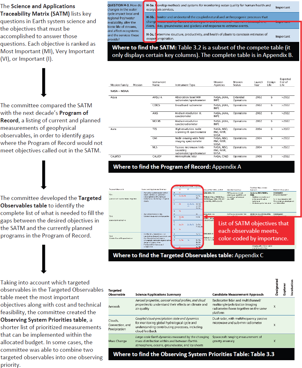
In addition, the committee is proposing an expansion of the Venture program elements to include a Venture-Continuity program element strand, focused on competitive opportunities for continuity observations with a goal of reducing cost. Candidates for the Venture-Continuity element could come from among Targeted Observables in Appendix C and Table 3.3, but are not explicitly identified as such. Each of these flight program elements is included in the funding wedge shown in Figure 3.4 and so can be implemented within anticipated resources. Details on these program elements, and the Targeted Observables to be implemented through them, are provided in the following text.
The seven Targeted Observables shown at the end of Table 3.3 were not allocated to any of the three program elements, but they are still considered important observations to implement in support of science and applications priorities identified in the SATMs. As the recommended flight program is implemented, it is expected that portions of the science for these unallocated observables will be addressed, particularly where similar measurement techniques are required to address both allocated and unallocated Targeted Observables. A more complete description of the disposition of these unallocated observables and the opportunities for pursuing their important underlying science is provided at the end of this section of the report.
The committee also recognizes that the focus on Targeted Observables, as opposed to missions and prespecified measurement approaches, does not lend itself to the consideration of multiple objectives being served by a single measurement technique. While this has the advantage of allowing for greater flexibility in implementation, it does not take full advantage of both the scientific and technical synergies that can develop from a more interdisciplinary framing. In particular, measurement technologies that address a particular Targeted Observable may likely also address others, and a careful evaluation of these opportunities should be built into the thinking and planning for flight program elements while respecting cost caps and guarding against mission creep leading to significant cost inflation.9 As NASA proceeds with planning for the implementation of the recommended flight program elements, the effort will benefit from input from a wide interdisciplinary community to help identify benefits and trade-offs among different measurement approaches. Possible interdisciplinary opportunities can be identified where observing techniques are common among Targeted Observables in Table 3.3. Lidar is highlighted as a clear example.
Recommendation 3.2: NASA should implement a set of space-based observation capabilities based on this report’s proposed program (which was designed to be affordable, comprehensive, robust, and balanced), by implementing its portion of the Program of Record and adding observations described in Table 3.3, “Observing System Priorities.” The implemented program should be guided by the budgetary considerations and decision rules contained in this report and accomplished through five distinct program elements:
- Program of Record. The series of existing or previously planned observations, which must be completed as planned. Execution of the ESAS 2017 recommendation requires that the total cost to NASA of the Program of Record flight missions from fiscal year (FY) 2018 through FY 2027—October 1, 2017 through September 30, 2027—be capped at $3.6 billion.
- Designated. A program element for ESAS-designated cost-capped medium- and large-size missions to address observables essential to the overall program, directed or competed at the discretion of NASA.
- Earth System Explorer. A new program element involving competitive opportunities for cost-capped medium-size instruments and missions serving specified ESAS-priority observations.
___________________
9 An example of both synergistic benefits and cost growth challenges is available through the lessons learned from the interdisciplinary scientific planning that emerged for the ESAS 2007 recommended Tier 2 Decadal Survey lidar mission known as the Aerosol/Cloud/Ecosystems (ACE) profiling lidar mission (ACE Science Study Team, 2016).
- Incubation. A new program element, focused on investment for priority observation capabilities needing advancement prior to cost-effective implementation, including an Innovation Fund to respond to emerging needs.
- EarthVenture. Earth Venture program element, as recommended in ESAS 2007, with the addition of a new Venture-Continuity component to provide opportunity for low-cost sustained observations.
The remaining text within this subsection, entitled “A Comprehensive Observation System,” elaborates on this Recommendation 3.2, including (in sequential order) discussions on the following:
- Summary of Observables.Table 3.3, which summarizes the Targeted Observables included in the recommendation and their allocation to flight elements.
- Prioritization Process. Description of the prioritization process used to identify the recommended Targeted Observables.
- Budget Considerations. An overview of how the recommendation is structured to meet budget constraints, including guidance for how to leverage the budget for an aspirational program.
- Observables Descriptions. Descriptions of the Targeted Observables included within each program element (Designated, Earth System Explorer, Incubation, Venture-Continuity).
- Opportunities for Non-Allocated Observables. Clarification of the opportunities available for unallocated Targeted Observables, including a case study for ocean science.
Prioritization Process
The Targeted Observables in Table 3.3 are responsive to the science and applications priorities (as measured by the Science/Applications Importance column) in Table 3.2, and ultimately to panel guidance addressing the science and applications as well as the needed observables. Table 3.2 was developed largely by the panels, but Table 3.3 was the responsibility of the steering committee without any direct panel consultation. Development of Table 3.3 from Table 3.2 involved two fundamental steps, listed here:
- Identify Observation Gaps. Identify those gaps in the POR corresponding to observables needed to address highest-priority science and applications objectives. In practice this meant working directly with two large tables of data. The first is the Program of Record table (Appendix A). The second is the Science and Applications Traceability Matrix (Appendix B). By comparing the two tables, a list was developed detailing gaps in observing capability (i.e., needed observations not available in the next decade’s POR) that are anticipated during the coming decade. The result of this effort was the Targeted Observables Table (Appendix C), which lists the 22 key unmet observation needs (referred to as Targeted Observables) in the next decade’s POR, as identified by the committee.
- Prioritize the Observation Gaps. Prioritization of the 22 Targeted Observables in Appendix C to derive the priorities in Table 3.3 was accomplished through extensive deliberation by the committee, with consideration of the following two factors:
- Scientific and Applications Priority. The scientific and applications priority is summarized in the Science/Applications Priorities column of the Targeted Observables table (Appendix C). The entries in this column refer to lines in the Science and Applications Traceability Matrix (Appendix B). At a simple level, priority can be discerned by the total number of Science and Applications Priorities, along with the preponderance of Most Important and Very Important priorities. While the committee used this simple view for guidance, decisions were made through direct review of the original science/applications priorities in Appendix B.
- Cost and Technical Feasibility. With the assistance of The Aerospace Corporation, various implementations were assessed to understand the potential cost and feasibility of measuring each proposed Targeted Observable. Because the committee is recommending observations, rather than missions, the assessment performs the role of an existence proof rather than an implementation plan. Nevertheless, a comprehensive range of feasibility factors was considered, from technical readiness to flight heritage.
The committee focused on ensuring that this process is traceable and grounded in the guidance of the panels. While endeavoring to achieve objectivity to the extent possible, the process inevitably involves subtle and often subjective trade-offs among the preceding factors. The committee held discussions involving complex considerations to arrive at the priorities in Table 3.3. An important consideration for the committee was the extent of interdisciplinary (i.e., Earth system) benefit obtained from a Targeted Observable, as measured by the degree of cross-panel prioritization. In addition, the committee considered programmatic balance (see Chapter 4 for a description of balance considerations) to be a desirable aspect of the recommended program.
While an inherent subjectivity exists in any prioritization, the multiple diverse perspectives from the steering committee that led to Table 3.3, as well as the consideration of panel input as informed by RFI responses, has produced a set of recommendations that is appropriately balanced, informed, and reflective of societal and scientific needs.
As also discussed elsewhere in this section, the committee chose to not simply list the prioritized Targeted Observables but to group them according to three candidate programmatic implementations (Designated, Earth System Explorer, and Incubation), based on the suitability of each Targeted Observable for each approach. In a general sense, the size of the resource commitment is justified by the value of the science and applications, as summarized for each Targeted Observable in the Science/Applications Priorities column of the Targeted Observables table (Appendix C). The committee’s overall goal was to maximize the amount and quality of the science and applications that can be achieved within constrained resources.
An example of the process is shown in Figure 3.4, illustrating the use of each of the key tables in development of the Aerosols Targeted Observable within Table 3.3.
Fitting Within a Realistic Budget
The committee had two fundamental strategic goals that guided its partitioning of the funds anticipated to be available for the Earth science program. The first goal is to achieve and preserve balance in the program portfolio by maintaining approximate ratios between each of the program elements. This is to be accomplished by application of the Decision Rules, which provide guidance on the cadence that elements in each program line should be implemented, as well as the possibility, if necessary, of modulating the schedule for development of the larger missions. The second goal is to control carryover into the next decade such that implementation of the large mission pipeline over the decadal boundary is maintained without deeply impacting the future funding wedge.
Figure 3.5 shows how the recommended program elements accomplish these two objectives and fit within the assumed profile of available funding.10 This budget assumes spending of $3.4 billion on new
___________________
10 Recognizing there is a natural latency that occurs at the transition between decadal surveys, it was assumed that there would be some encumbrance beyond 2027 to complete this decadal survey’s recommended program. The encumbrance equates to approximately all of the assumed available flight funding in 2028 (the first year post transition), falling to half and then less than a quarter of assumed available flight program funding in the second and third post-transition years, respectively. This approach, if followed for each successive decade, will ensure a full mission pipeline while also facilitating an earlier start for subsequent decadal surveys’ priorities.
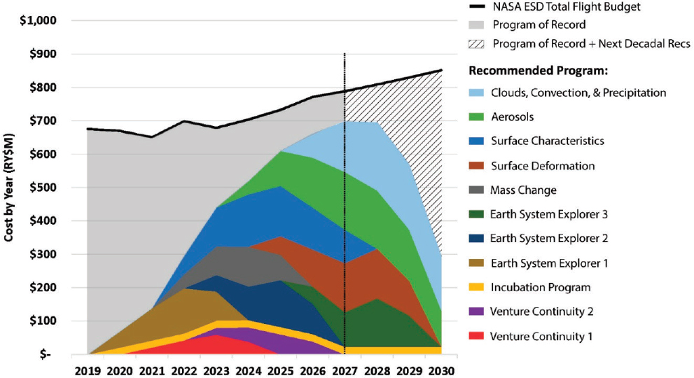
programs (beyond the already allocated POR runout budget) during the coming decade, and a lien on the following decade of $1.7 billion due to flight programs starting late in the decade. Such liens are an accepted consequence of achieving continuity from one decadal study recommendation to the next, but minimizing the lien is desirable (NRC, 2015b). The lien proposed by ESAS 2017 is less than half of the $3.6 billion lien currently estimated to complete POR flight programs this coming decade that were started last decade.
As described in more detail in the remainder of this chapter, the recommended program includes funding for the following:
- Designated. Three large (two expected to be <$800 million in FY 2018, one expected to be <$650 million) and two medium (one expected to be <$300 million and the other expected to be <$500 million) cost-capped projects, directed or competed at the discretion of NASA.
- Earth System Explorer. Three competitively selected cost-capped (<$350 million) projects.
- Venture-Continuity. Two projects that are <$150 million each, selected competitively with a goal of reducing costs as compared to prior projects for the same observable.
- Incubation. Funded at $20 million per year to advance identified priorities for concept and technology maturation, including the Innovation Fund to enable program-level innovation.
Given the breadth of observations needed to address priorities in Earth system science and the expectation of comparatively austere budgets, the recommended program relies on competition as the core approach to controlling individual mission costs, through the use of cost caps combined with trades between performance and risk during the formulation and implementation stages of system development.
An Aspirational Program
The committee intended the proposed observing system to be realistically accomplished within nominal budget growth, with recommended investments stated in terms of the “maximum recommended NASA development cost” levels to ensure that program balance is maintained.11
For each program element, the included Targeted Observables were drawn from the nonprioritized list of Targeted Observables identified in Appendix C, and intended to address the science and applications priorities listed in that table. In order for implementations of Targeted Observables to remain within their respective cost caps, however, it is not expected that every science and applications priority identified in Appendix C will be achieved for each relevant Targeted Observable. Rather the implementation is expected to first target the highest currently unmet science and applications priorities, and address others as feasible.
That should not preclude NASA from trying to accomplish more, and the committee believes that NASA can and should do so. Indeed, the new Earth System Explorer program includes more than twice as many candidate observations as the committee believes will be implemented in this decade, and Appendix C suggests there are many more good candidates for flight opportunities such as Earth Venture. With an increased budget, an aspirational program could be pursued. More importantly, however, it is possible to be aspirational within the nominal budget—to get more done with the same amount of resources. NASA is quite adept at many of the ways this could happen, as shown here:
- International partnerships that provide the same capability with reduced cost to NASA. Interest by several viable international partners was expressed to the committee regarding potential collaboration opportunities. Several of the priority observations included in the system are known to also be high priorities of these international partners, leading the committee to believe that partnering opportunities are quite promising.
- Technology innovation with the potential to reduce cost for all aspects of space-based observation. The commercial sector (in addition to NASA and academia) is presently introducing a wide range of technology innovation capabilities with the potential to be leveraged by NASA for cost reduction.
- Programmatic innovation, including public-private partnerships and spacecraft block buys, that accomplish the same goals with reduced resources.
- Aggressive cost management and requirements control of programs being implemented.
- Extended operations for continuity observations that delay the need for new missions.
A comprehensive effort within NASA focusing on these steps could reduce cost and generate the additional resources needed to expand the Earth System Explorer program element, complete the survey’s high-priority observations more rapidly, or increase opportunities for continuity of key Earth system observations. Doing so would enable additional high-priority science beyond the baseline recommended
___________________
11 The maximum recommended NASA development cost is what is allocated from NASA’s budget to cover the prelaunch (development phase) and launch vehicle cost for a mission to address the stated science and applications objectives. Development phase costs include reserves. Operations cost and associated research and analysis (R&A) funding are not included in this total.
by this committee. The key to achieving this aspirational program relies on managing costs through the approaches outlined in items 1 through 5 in the preceding list, and incentivizing mission development to be accomplished as far below the cost cap as possible.
Recommendation 3.3: NASA should manage development costs for each flight program element (including the Program of Record committed to prior to this report), and for each project within the Designated program element, so as to avoid impact to other program elements and projects.
- Innovative cost reduction, through programmatic or technological advances and partnerships, should be sought and incentivized where possible.
- By the time of the Midterm Assessment, NASA should report on steps it has taken (e.g., use of innovative approaches or partnerships) to ensure cost-effective development in each program element, and if or how these steps translate to increased science opportunity across the program.
- NASA should consult its standing scientific advisory committees if the project cost of the Program of Record is expected to grow to consume more than $3.6 billion in the FY 2018-2027 decade, if more than one mission in this decadal survey is delayed more than 3 years, or upon premature loss of a mission in the Program of Record or one required to make the measurements of this decadal survey.
- When appropriate, cost-effective, and consistent with recommended cost caps, NASA should consider instrument and mission designs that can increase science/applications return by combining Targeted Observables having common measurement technologies.
Program Element: Designated
The Designated program element represents a group of Targeted Observables believed by the committee to be of sufficiently high value to the Earth system science and applications communities to warrant designated implementation during the decade. This implementation could occur through directed guidance to the NASA Centers, through internal or external competition, or other means chosen by NASA ESD to achieve the most cost-effective solution.
Within the Designated program element, five Targeted Observables are recommended for implementation during the 2017-2027 decade. Table 3.5 lists these and indicates the maximum recommended NASA development cost, with science and implementation considerations discussed for each in the following sections. The maximum recommended development costs are not to be taken as expected development costs. Instead, the committee expects NASA to identify implementation approaches that achieve the recommended objectives for less than the identified maximum.
CATE Cost Confirmation
Consistent with other NASA space science decadal surveys, The Aerospace Corporation CATE process was applied to all concepts expected to cost more than $500 million, excluding operations costs.12 For those expected to be less than $500 million, a cost analysis was performed to estimate a cost cap but no formal CATE was completed. For the three large (two <$800 million, one <$650 million) Targeted Observables in Table 3.5, notional proof-of-concept missions with the recommended capabilities were evaluated to ensure top-level technical and programmatic risks were understood. Aerospace found each of these proof-of-concept missions to be implementable within the listed cost cap.
___________________
12 As discussed earlier in this chapter, the Cost Assessment and Technical Evaluation (CATE) process is a formal cost and technical readiness evaluation, performed by The Aerospace Corporation. It is mandated for the decadal survey.
TABLE 3.5 Targeted Observables to Be Addressed Through the Designated Program Element, and Their Respective CATE-Confirmed or Estimated Cost Caps
| Targeted Observable | Cost Cap ($FY2018) | Basis for Being Foundational |
|---|---|---|
| Aerosols | CATE Cap $800 million | Essential for air quality forecasting; provides critical insights into key radiative forcings, both direct and indirect (from cloud hydrometeor size and optical depth). When combined with Clouds, Convection, and Precipitation observations, enables assessment of aerosol effects on clouds and precipitation. Addresses many of the “Most Important” objectives of the Climate Panel and Weather and Air Quality Panel, along with key components of the water and energy cycle integrating theme. |
| Clouds, Convection, and Precipitation | CATE Cap $800 million | Critical for assessing low and high cloud feedbacks, and seasonal and interannual climate variability and its prediction, processes that are at the core of severe weather and extremes. Fundamental observations for water resource and hydrological applications. When combined with Aerosols observations, aerosol indirect effects can also be substantially advanced. Addresses many of the “Most Important” objectives of the Climate, Weather and Air Quality, and Hydrology panels, along with key components of the Water and Energy Cycle and Extreme Events integrating theme. |
| Mass Change | Estimated Cap $300 million | Ensures continuity of measurements of groundwater and water storage mass change, land ice contributions to sea-level rise, ocean mass change, ocean heat content (when combined with altimetry), glacial isostatic adjustment, and earthquake mass movement. Also important for operational applications, including drought assessment and forecasting, hazard response, and planning water use for agriculture and consumption. Addresses various “Most Important” objectives of the Climate, Hydrology, and Solid Earth panels and key components of the Water and Energy Cycle integrating theme. |
| Surface Biology and Geology | CATE Cap $650 million | Key to understanding active surface changes (eruptions, landslides, and evolving landscapes); snow and ice accumulation, melting, and albedo; hazard risks in rugged topography; effects of changing land use on surface energy, water, momentum, and carbon fluxes; physiology of primary producers; and functional traits and health of terrestrial vegetation and inland and near-coastal aquatic ecosystems. Further contributes to managing agriculture and natural habitats, water use and water quality, and urban development as well as understanding and predicting geological natural hazards and land-surface interactions with weather and climate. Depending on implementation specifics, the Targeted Observable may also contribute to hyperspectral open-ocean observation goals. Addresses many “Most Important” objectives of the Ecosystem, Hydrology, and Solid Earth panels, and addresses key components of the Water and Energy Cycle, Carbon Cycle, and Extreme Events integrating themes. |
| Surface Deformation and Change | Estimated Cap $500 million | Critical for assessing ice sheet stability and the potential for ice sheets to make large rapid contributions to sea-level rise. Key to mapping surface strain rates in order to understand earthquakes, volcanoes, landslides, and sea-level rise. Enables monitoring of tectonic plate deformation, changes in groundwater and subsidence, and thawing of permafrost. Directly addresses six “Most Important” and four “Very Important” objectives of the Earth Surface and Interior Panel, as well as one or more “Most Important” objectives of the Hydrology and Climate panels. Provides important insights into various components of the Water and Energy Cycle, the Carbon Cycle, and the Extreme Events integrating themes. |
NOTE: These are listed in alphabetical order, with proposed development sequencing discussed in the text.
The CATE process is by its very nature conservative (NRC, 2015b). It does not, for example, incorporate innovative implementation approaches or account for partnership opportunities that have the ability to significantly lower the cost of implementation to NASA. For large (>$500 million) Targeted Observables listed in Table 3.5, the CATE process identified this cap as a cost category limit within which the observable could be implemented at acceptable risk. The actual estimated cost was always below the cost cap, suggesting the realistic expectation that each implementation can be completed for less than the cost cap values in Table 3.5 (potentially considerably less).
Implementation Sequence
Based on the relative costs and risks of the three higher-cost Targeted Observables, and the substantial synergy gained by obtaining overlap between the Aerosols and Convection and Precipitation Targeted Observables, the committee suggests that the order of implementation be (1) Surface Biology and Geology, (2) Aerosols, and (3) Clouds, Convection, and Precipitation. However, if opportunities present themselves that in NASA’s judgment allow for a more effective implementation (through lower costs, better technologies, etc.), this implementation sequence should be flexible in order to be responsive to such opportunities. One reason for choosing the suggested sequencing is that cost-reducing opportunities, such as international partnerships, are particularly viable for Targeted Observables implemented late in the survey interval.
Cost Control
To further protect program balance, the committee expects that NASA will manage the Targeted Observables within the Designated program in such a way that the implemented missions adhere to their costs caps and do not adversely affect other elements of the flight program. To achieve this, the progress with developing and implementing these missions should be reviewed during the Midterm Assessment. The advantage of ensuring cost-effective investments, to NASA and its science/applications programs, is clear. When implementation can be achieved below the stated allocation (e.g., through innovative program implementation, partnerships, or other means), program breadth may be increased to address other identified priority observations consistent with the decision rules provided in Chapter 4.
Designated Targeted Observables
Each of the Targeted Observables in Table 3.5 recommended for the Designated program element is discussed in the following text, with Targeted Observables presented in alphabetic order.The extent to which science and applications objectives of multiple panels are addressed within each Targeted Observable demonstrates the cross-disciplinary nature of the program.
Aerosols
| Earth Science/Applications Objectives for the Designated Targeted Observable: Aerosols | |||
|---|---|---|---|
| Most Important | Very Important | Important | |
| Hydrology | 1c | 2b | |
| Weather | 1a, 2a, 5a | 6a, 9a, 10a | |
| Ecosystems | |||
| Climate | 2a, 2h | 2g, 5a, 5c, 7a | 3d, 4d, 5b, 5d, 7b, 8g, 9a |
| Solid Earth | 1a | ||
The Aerosols Targeted Observable corresponds to a combination of TO-1 and TO-2 in the Targeted Observables Table (see Appendix C). The IPCC 2013 Climate Change Assessment Report determined that uncertainties associated with aerosols and aerosol-cloud interactions are the largest radiative forcing uncertainty. Because of this, knowledge of their characteristics and processes is critical to reducing the uncertainty of future projections of climate change. As a result, aerosol observations are one of the higher priorities from the Climate Panel. In addition, the health effects from pollution are the largest environmental risk, and therefore aerosols are one of the most important boundary layer properties identified by the Weather Panel as essential both for air quality forecasting and for connecting health effects with pollution. Finally, aerosols, through their alteration of direct and diffuse radiation, change the amount of radiation available to ecosystems. The considered implementation of a backscatter lidar and multiangle, multispectral polarimeter would address important inputs for aerosol direct radiative forcing, and provide information that partially addresses indirect effects through aerosol effects on cloud hydrometeor size and cloud optical depth. These radiative forcings are a significant source of uncertainties in climate model projections. In combination with the Clouds, Convections, and Precipitation Targeted Observable, it would also address the additional aspects of the aerosol indirect effect (on clouds and precipitation formation), thus accomplishing key objectives of the ESAS 2007 recommended ACE mission.
- Science Considerations. Aerosol measurements are essential elements for understanding climate forcings and feedbacks. The types of systems that would contribute profiling (lidar) would also be capable of detecting height and optical properties of high thin clouds and cloud properties of lower thicker clouds, providing important information for cloud feedbacks in the climate system. In addition, such observations would provide information, critical for air quality forecasting, about aerosol profiles in the boundary layer. The information on clouds and aerosols would yield additional insights into cloud processes and processes that affect precipitation, particularly when Aerosols is flown simultaneously with a system for observing cloud, convection, and precipitation. As such, this observing system spans climate, weather, and air quality and directly maps to the water and energy cycles integrating themes.
- Candidate Measurement Approaches. The candidate measurement approach considered includes a lidar and a polarimeter. Expected lidar measurement implementations will provide aerosol extinction profiles and cloud top heights as well as vertical profiles of cloud occurrence in thinner clouds. The polarimeter provides aerosol/cloud properties information supporting science and applications objectives related aerosol/particulate matter optical depth, particle size, and some information on speciation. It also provides cloud optical depths and cloud droplet size (in the uppermost layer near cloud tops) and can distinguish between spherical cloud drops and nonspherical ice particles. The polarimeter also provides column-integrated information on aerosols that could be used to constrain lidar extinction profile estimates. Depending on implementation specifics, a lidar may also contribute to aquatic ecosystem structure, ocean mixed layer depth, ice-sheet topography, land topography, and PBL height. In particular, many of the scientific and technical opportunities and challenges for a joint aerosol-ocean measurement system have been mapped out in some detail as part of the planning for the ESAS 2007 Aerosol/Cloud/Ecosystems (ACE) mission (ACE Science Study Team, 2016). The recovery of upper-ocean plankton profiles from the Cloud-Aerosol Lidar with Orthogonal Polarization (CALIOP) sensor indicates that, with appropriate consideration, the Aerosol Targeted Observable should also be able to address key aspects of the Ocean Ecosystem Targeted Observable TO-10 (Appendix B) and the associated high-priority science and applications objectives from the Ecosystem, Weather, and Climate panels (W-3a, E-1b, E-3a, C-2d, and C-8d).
- The Aerosol Targeted Observable instrument and mission design, therefore, should seek to address these interdisciplinary objectives while recognizing that the primary mission focus is meeting the aerosol science objectives as described and remaining within the cost cap. Opportunities should be assessed to determine the extent to which these additional science goals can be achieved while also meeting the aerosol science objectives and maintaining overall costs at or below the recommended cost cap.
- CATE Evaluation. The CATE evaluation considered a reference concept consisting of a backscatter lidar and polarimeter. It found that the concept is based on mature technology and is consistent with a cost cap of $800 million or less (excluding operations). High Spectral Resolution Lidar (HSRL) was a desired capability as part of Aerosols, but cost and technical readiness considerations suggested it was incompatible with the recommended Aerosols cost cap.
- Descope Options. In the event development costs are expected to exceed the $800 million cost cap, the TO-1 and TO-2 Target Observables (Appendix C) could be instead included separately as candidates within the Earth System Explorer competition, using the available budget to fund two additional Earth System Explorer solicitations. This is preferred over descoping Aerosols to just one of the two (lidar and polarimeter) measurement techniques or to proceeding with a higher cost for the combined implementation.
- POR Assumptions. There are no dedicated atmospheric lidars in the POR after EarthCARE, which is expected to end in about 2022. The POR includes polarimetry from the European 3MI (Multi-viewing, Multi-channel, Multi-polarization Imager) instrument. Multiangle polarimetry will be provided by the Multi-Angle Imager for Aerosols (MAIA), but this measurement has limited coverage.
- Partnerships. NASA is encouraged to seek commercial or international partnership opportunities with the goal of reducing implementation costs and enabling overlap between the Aerosol and Clouds, Convection, and Precipitation efforts.
- Budgetary Guidance. In keeping with the guidelines of the Designated program element and this report’s Recommendation 3.3, the Aerosols Targeted Observable has a maximum recommended development cost of $800 million (in $FY2018).
Clouds, Convection, and Precipitation
| Earth Science/Applications Objectives for the Designated Targeted Observable: Clouds, Convection, and Precipitation | |||
|---|---|---|---|
| Most Important | Very Important | Important | |
| Hydrology | 1a, 1b, 1c | 3b, 4b | |
| Weather | 1a, 2a, 4a | 3a | 9a, 10a |
| Ecosystems | 3a | ||
| Climate | 2a, 2h | 2g | 3f, 5d, 7e, 8h |
| Solid Earth | 1c | 4b | |
The Clouds, Convection, and Precipitation Targeted Observable corresponds to TO-5 in the Targeted Observables table (Appendix C). Measurements associated with TO-5 are essential to advance understanding and prediction of cloud feedbacks, moist convection and its influence on weather and extremes, and the processes of precipitation, including important modes of precipitation not addressed within the POR. The Clouds, Convection, and Precipitation Targeted Observable also addresses priorities that emerged across multiple panel recommendations and from considerations of broader Earth science integration as, for example, described in the prior discussion of integrating themes.
Precipitation measurements and, notably, the combined information on cloud and precipitation processes to be addressed by the proposed measurements, are fundamental for addressing the high priorities of the Hydrology Panel, cloud feedbacks identified in the Climate Panel, and important topics on weather extremes. When combined with other measurements, such as those proposed to address the Aerosols Targeted Observable, other important objectives such as those associated with aerosol indirect effects can also be advanced.
TO-5 is motivated to address widely recognized critical challenges within Earth sciences. Clouds are a principal source of uncertainty in projections of climate change (IPCC, 2013, Assessment). These uncertainties are associated with low and high cloud feedbacks as described in the report from the Climate Panel (Chapter 9), and to the process of moist convection, which is a central theme of the cloud-climate sensitivity grand challenge of the World Climate Research Programme (WCRP,13 Bony et al., 2015). Moist convection is also central to two high-importance weather priorities, being the essential building block of our major storm systems found throughout the tropics and midlatitudes. Convective storms are the sole source of precipitation in many regions of our planet and are major sources of severe weather and extreme precipitation. Measurements of the vertical distribution of cloud and precipitation properties, including measurements of water and ice contents, and other microphysical information, are essential for quantifying the processes that underpin the challenges of the Clouds, Convection, and Precipitation Targeted Observable and for better predicting the intensity of storms and extreme weather.
- Science Considerations. This observation will address science and applications goals related to cloud cover (with the assistance of the POR) and cloud property profiles (with the assistance of the POR and/or the Aerosols Targeted Observable), precipitation profiles, precipitation (including light rain and snowfall), diurnal cycle of precipitation (with the assistance of the POR), convective vertical motion or proxies of it, and cloud water and ice contents. When cloud and precipitation observations overlap with the aerosol measurements earlier, they can better address the aerosol indirect effect priority called out by the Climate Panel as high importance. This measurement is also a central component of the ACE mission identified in ESAS 2007. A short-pulse altimeter mode of operation of higher frequency radar could help measure snow depth on the ground, which is an important priority both of hydrology and to ice mass measurement objectives, though this capability should not be allowed to drive mission cost or complexity.
- Candidate Measurement Approaches. The expected radar measurements will provide joint cloud water and ice contents, rain and snow amounts, and Doppler motions within clouds and convection. The radar will also provide profiles of shallow and deep clouds and some information on microphysical properties through the combination of frequencies and Doppler. The radar is expected to be a dual frequency W-/Ka-band system. If the W-band radar includes an altimeter mode, it could also contribute to surface snow depth measurement needs; however, adding an altimeter mode to the W-band radar is not considered a priority and thus is not recommended if it drives cost. Cloud optical properties and diurnal cycle information will come from the POR observations of clouds from available advanced geostationary imaging radiometers. Time and spatial coverage of precipitation similarly relies on the microwave radiances data within the POR, and diurnal cycle coverage of precipitation could be anticipated if this POR is augmented in decade.
- CATE Evaluation. The CATE evaluation of a reference concept consisting of a dual-band radar building on CloudSat heritage found that the concept is based on mature technology and has the potential to be executed within a cost cap of $800 million or less (excluding operations). Recent
___________________
13 See the World Climate Research Program’s Grand Challenges website at http://www.gewex.org/about/science/wcrps-grand-challenges/, accessed August 9, 2017.
- technological advances have led to either miniaturized or greatly simplified microwave radiometers and radar systems, suggesting the possibility of leveraging technology innovation and miniaturization to achieve the selected goals at reduced cost. These innovations are seen in for example, Raincube (Radar in a CubeSat), the demonstration of Compact Ocean Wind Vector Radiometer (COWVR; Brown et al., 2016), and in the implementation of the Time-Resolved Observations of Precipitation Structure and Storm Intensity with a Constellation of Smallsats (TROPICS) and Temporal Experiment for Storms and Tropical Systems (TEMPEST) EV-I missions.
- Descope Options. In the event development costs exceed the maximum NASA development cost level recommended here, the radar can be descoped to a single band, retaining Doppler capability.
- POR Assumptions. Addressing this Targeted Observable requires fully leveraging missions in the POR and augmenting them with new measurements that offer a dimension of time and motion as a way of quantifying and understanding processes. New observations of the dynamical aspects of cloud, convection, and precipitation processes will place those processes within the context of global mapping of precipitation and its diurnal cycle. Cloud properties (such as cloud amount, optical depth, and particle size) are available from the spectral radiance measurements provided by MODIS and VIIRS on polar orbiting satellites that are assumed within the POR. The same information can now be extracted from the advanced imagers available from the current and planned constellation of operational geostationary satellites. Precipitation radar measurements from GPM are assumed within the POR, but higher latitude precipitation is not addressed within the POR after CloudSat and EarthCARE. Cloud profile data from CloudSat and CALIPSO will not be available in the decade, while EarthCARE will be available only in the early part of the decade. Precipitation information especially over ocean relies heavily on microwave imaging radiometer measurements, and the time/space coverage of this information will not be available in the coming decade (see Box 4.4, in Chapter 4).
- Partnerships. NASA is encouraged to seek commercial or international partnership opportunities with the goal of reducing implementation costs and enabling overlap between the Aerosol and Clouds, Convection, and Precipitation efforts. In particular, NASA is encouraged to assess the extent to which the three series of operational microwave radiometers that will be flying concurrently later in the coming decade—EUMETSAT/EPS-2G-B, USAF/WSF, and CMA FY-3—can contribute toward meeting the objectives of this mission.
- Budgetary Guidance. In keeping with the guidelines of the Designated program element and this report’s Recommendation 3.3, the Clouds, Convection, and Precipitation Targeted Observable has a maximum recommended development cost of $800 million (in $FY2018).
Mass Change
| Earth Science/Applications Objective for the Designated Targeted Observable: Mass Change | |||
|---|---|---|---|
| Most Important | Very Important | Important | |
| Hydrology | 1a, 2c | 3b, 4c | |
| Weather | |||
| Ecosystems | |||
| Climate | 1a, 1b, 1c | 1d | 7d, 7e |
| Solid Earth | 1b, 3a, 4a | 5a | 6b |
The Mass Change Targeted Observable corresponds to TO-9 in the Targeted Observables table (Appendix C). The movement of mass, whether it is moisture, groundwater, snow, ice, ocean water, and so on represents exchanges within and across elements of the Earth system. As such, the Mass Change Targeted Observable provides an integrated view of the entire physical Earth system, and allows the relating of changes in one system component to changes in another. By providing continuity of the GRACE measurement record, it addresses Most Important and Very Important objectives for three panels (Climate, Hydrology, and Solid Earth) and contributes to several integrating themes.
- Science Considerations. This Targeted Observable will ensure continuity of information on groundwater and water storage mass change, land-ice mass change, ocean mass change, glacial isostatic adjustment, and earthquake mass movement. When combined with altimetry, additional information on heat storage is obtained. Gravity-derived measurements of mass change, as have been shown by GRACE, address key objectives related to sea-level rise, ocean heat content (Box 3.7), terrestrial water storage, among others. Consequently, monitoring changes and movement of mass throughout the Earth integrates objectives of the Climate, Solid Earth, and Hydrology panels, as well as addressing key integrating themes such as water and energy cycle with linkages to assessing whether or not systems may be approaching thresholds or tipping points, and assessing trends in the parameters observed, especially given the continuity of mass change and gravity measurements since the launch of GRACE in 2002.
- Candidate Measurement Approaches. The GRACE gravity observation can be accomplished through either of two ranging techniques (microwave and optical) that are being evaluated as part of the GRACE-FO mission. Either approach provides bulk measurements of mass fluctuations that are primarily associated with water changes within the Earth system. A down-select to a single measurement technology is likely required to fit within the allocated investment level. These measurements provide a way to track bulk changes in terrestrial water, changes to ice mass, and ocean water mass. Although these measurements are coarse in scale, making their use in water resource management challenging, they provide valuable insights on how water in bulk form cycles through and the changes within the Earth system. When this information is augmented with the ocean altimeter observations of the POR and in situ data from ARGO floats, then additional but important information about ocean heat storage is obtained. Monitoring this energy change over time is fundamental for assessing the state of the Earth system and its future evolution.
- CATE Evaluation. Cost and technical evaluation of a notional mission concept similar to the original GRACE mission found the concept to be technically mature with costs that are well understood, supporting a low-risk implementation recommendation.
- Descope Options. No descope options have been identified.
- POR Assumptions. The POR includes mass change measurements from GRACE-FO and continued altimetry measurements from the JASON and Sentinel-6 missions.
- Partnerships. NASA is encouraged to seek international partnership opportunities to implement this mission, and to phase implementation to ensure flight readiness prior to the end of the GRACE-FO mission.
- Budgetary Guidance. In keeping with the guidelines of the Designated program element and this report’s Recommendation 3.3, the Mass Change Targeted Observable has a maximum recommended development cost of $300 million (in $FY2018).
Surface Biology and Geology
| Earth Science/Applications Objectives for the Designated Targeted Observable: Surface Biology and Geology | |||
|---|---|---|---|
| Most Important | Very Important | Important | |
| Hydrology | 1c | 2a, 4a | 2b, 3a, 3b, 3c, 4c, 4d |
| Weather | 3a | ||
| Ecosystems | 1c, 2a, 3a | 1a | 1d, 5a, 5b, 5c |
| Climate | 3a | 3c, 3d, 6b, 7e, 8f | |
| Solid Earth | 1a | 1c, 2b | 4b, 4c, 7a |
The Surface Biology and Geology Targeted Observable, corresponding to TO-18 in the Targeted Observables table (Appendix C), enables improved measurements of Earth’s surface characteristics that provide valuable information on a wide range of Earth System processes associated with geological dynamics and terrestial and marine ecosystem changes. Society is closely tied to the land surface for habitation, food, fiber, and many other natural resources. The land surface, inland, and near-coastal waters are changing rapidly due to direct human activities as well as natural climate variability and climate change. New opportunities arising from enhanced satellite remote sensing of Earth’s surface provide multiple benefits for managing agriculture and natural habitats, water use and water quality, and urban development, as well as understanding and predicting geological natural hazards. The Surface Biology and Geology observable is linked to one or more Most Important or Very Important science objectives from each panel and feeds into the three ESAS 2017 integrating themes: water and energy cycle, carbon cycle, and extreme events.
- Science Considerations. This Targeted Observable will likely be addressed through hyperspectral measurements that support a multidisciplinary set of science and applications objectives. Visible and shortwave infrared imagery addresses multiple objectives: active surface geology (e.g., surface deformation, eruptions, landslides, and evolving landscapes); snow and ice accumulation, melting, and albedo; hazard risks in rugged topography; effects of changing land use on surface energy, water, momentum and carbon fluxes; physiology of primary producers; and functional traits of terrestrial vegetation and inland and near-coastal aquatic ecosystems. Thermal infrared imagery provides complementary information on ground, vegetation canopy, and water surface temperatures as well as ecosystem function and health. Depending on implementation specifics, the Targeted Observable may also contribute to hyperspectral open-ocean observation goals. However, such goals are met to a large degree by POR elements, in particular the hyperspectral PACE mission, and are not considered a priority for additional implementation (and thus are not recommended if they drive cost). Observations of the Earth’s surface biology and geology, with the ability to detect detailed spectral signatures, provide a wide range of opportunities for Earth system science parameters across most of the panels and integrating themes. As such, this Targeted Observable maps to some of the highest panel priorities as well as the Integrating Themes.
- Candidate Measurement Approaches. High spectral resolution (or hyperspectral) imagery provides the desired capabilities to address important geological, hydrological, and ecological questions, building on a successful history of past and ongoing multispectral remote sensing (e.g., MODIS). Consequently, hyperspectral imagery with moderate spatial resolution (30-60 m) is identified as a priority for implementation.
- CATE Evaluation. The CATE evaluation considered the Hyperspectral Infrared Imager (HyspIRI) concept, which was developed by NASA Science Mission Directorate following a recommendation
- from the 2007 ESAS decadal survey, and found that the concept is technically mature and costs are well-understood, supporting a recommendation for early implementation.
- Descope Options. In the event costs exceed the maximum recommended here, relaxing instrument requirements or eliminating the Thermal Infrared Radiometer (TIR) instrument is advised.
- POR Assumptions. It is assumed that the Sustainable Land Imaging program continues to provide Landsat-class land imagery to complement the measurements described here.
- Budgetary Guidance. In keeping with the guidelines of the Designated program element and this report’s Recommendation 3.3, the Surface Biology and Geology Targeted Observable has a maximum recommended development cost of $650 million (in $FY2018).
Surface Deformation and Change
| Earth Science/Applications Objectives for the Designated Targeted Observable: Surface Deformation and Change | |||
|---|---|---|---|
| Most Important | Very Important | Important | |
| Hydrology | 1c, 2c | 4a | 4b |
| Weather | |||
| Ecosystems | |||
| Climate | 1c | 7b, 8f | |
| Solid Earth | 1a, 1b, 2a, 3a, 3b, 4a | 1c, 2b, 2c, 5a, 6a | 4b, 6b, 6c, 6d, 7a |
The Surface Deformation and Change Targeted Observable corresponds to TO-19 in the Targeted Observables table (Appendix C). By monitoring the physical dynamics of Earth’s surface, we increase our ability to anticipate devastating geologic hazards, and monitoring progressive surface deformation can reveal how Earth’s systems are changing either naturally or through human activity. Such monitoring is key to avoiding surprises and improving our ability to anticipate future Earth states. This Targeted Observable is cited by nearly all of the Earth Surface and Interior objectives; it also matches needs expressed by the Hydrology Panel and the Climate Panel.
- Science Considerations. The Targeted Observable will provide surface deformation measurements including surface change monitoring, ice-sheet dynamics, the Antarctic grounding line migration, and permafrost thaw derived from subsidence. The measurements support science and applications objectives related to earthquakes, volcanoes, landslides, sea level, plate tectonics, the cryosphere, and groundwater. InSAR also is applicable to examining terrestrial ecosystem structure (Treuhaft et al., 2004). Measurements of displacement and surface deformation capture many of the Most Important and Very Important objectives of the Solid Earth, Hydrology, and Climate panels. Moreover, the more than 25-year history of InSAR observations of deformation and displacement establishes a long history of displacement observations, enabling detections of trends in behavior of land and ice processes.
- Candidate Measurement Approaches. The presumed measurement implementation involves Synthetic Aperture Radar (SAR) and Interferometric SAR (InSAR). SAR and InSAR have wide application across Earth science, including detection and monitoring of ice-sheet motion and grounding line locations, which are critical for assessing stability of ice sheets and their potential to cause rapid sea-level rise; detection of ground motion from earthquakes; detection of surface deformation and eruptive products of the active volcanoes; and mapping of landslides. Consequently, providing
- surface deformation measurements with improved space-time coverage post-NISAR was identified as a priority for implementation.
- CATE Evaluation. The recommended cost level does not support InSAR continuity through a reflight of a NISAR-like mission. Instead, continuity is to be pursued through consideration of international partnerships or a constellation of small satellites with relaxed performance characteristics to provide for the desired continuity within the specified NASA cost level. The decade’s priority science and applications objectives suggest that implementation should consider reduced spatial resolution in favor of improved temporal resolution, which further enables innovative implementation approaches (i.e., smaller aperture requirements imply the possibility of smaller satellites and lower cost).
- Descope Options. Should the maximum NASA development cost recommended here prove insufficient, the committee does not recommend a higher-cost implementation. Instead, the funding should be used to allow one additional Earth System Explorer competition and the Surface Deformation and Change Targeted Observable made eligible for competition in that flight program element.
- POR Assumptions. The POR includes NISAR, which is currently planned to launch in late 2021 and is designed to operate for 3-5 years, with no planned follow-on. NISAR’s primary science requirements are crustal deformation, glacier and ice-sheet motion, biomass structure, and sea-ice dynamics. NISAR operates at L-band, and can also look left to view Antarctica, for ice-sheet monitoring. It will have a dual-frequency ionospheric correction to enable improved detection of slow solid Earth signals.
- Partnerships. NASA is encouraged to seek international partnership opportunities to implement this mission, and to phase implementation to follow the NISAR mission. If the NISAR mission launch date slips, implementation of this mission may also move to the right.
- Budgetary Guidance. In keeping with the guidelines of the Designated program element and this report’s Recommendation 3.3, the Surface Deformation and Change Targeted Observable has a maximum recommended development cost of $500 million (in $FY2018).
Program Element: Earth System Explorer
To improve programmatic responsiveness while also maximizing the role of competition in implementing flight recommendations, a new medium-class (<$350 million FY 2018) cost-capped solicitation is recommended. The Earth System Explorer would be aimed at addressing the specific list of observing system priorities identified in Table 3.3 and summarized in Table 3.6 (no relative priorities are assigned to the candidates in the list).
The new Earth System Explorer line consists of a set of competitively selected principle investigator (PI)-led missions intended to mirror the proven success of the Astrophysics and Heliophysics Medium Class Explorer (MIDEX)14 lines. This program is designed to accomplish high-quality Earth system science investigations addressing one or more priority Targeted Observables in Table 3.6, utilizing innovative, streamlined, and efficient management approaches that seek to contain mission cost through commitment to, and control of, design, development, and operations costs. Analogous to MIDEX, specific mission objectives are defined by the PIs in their proposals and approved by NASA through confirmation review.15
___________________
14 Medium Class Explorer (MIDEX) spacecraft generally include selective redundancy with a cost in the range of $60 million to $85 million, depending on attitude control performance, communication requirements, and the need for propulsion. Launch costs are generally in the range of $55 million. MIDEX missions typically consist of a 250 kg payload (approximately 100 kg for instruments and 150 kg for the spacecraft) launched on a Pegasus-class vehicle to orbit.
15 While Table 3.3 lists the observing system priorities to be addressed in proposals to Earth System Explorer solicitations, the scope and technical requirements, and thereby the extent to which any particular objective associated with a Targeted Observable is met, depend on the proposed implementation approach, which will be assessed as part of the competitive selection process.
TABLE 3.6 Targeted Observables to Be Addressed Through the Competitive Earth System Explorer Program Element
| Targeted Observable | Implementation Considerations |
|---|---|
| Atmospheric Windsa | Address all or part of TO-4. Active sensing (lidar, radar, scatterometer); passive imagery or radiometry-based atmospheric motion vectors (AMVs) tracking; or lidar.b |
| Greenhouse Gases | Address all or part of TO-6. Can be active or passive, global or regional; or lidar.b |
| Ice Elevation | Addresses all or part of TO-7. Lidar;b if CryoSat-3 not approved, then highest-priority function for multifunction lidar. |
| Ocean Surface Winds and Currents | Address all or part of TO-11. Doppler scatterometer. |
| Ozone and Trace Gases | Address all or part of TO-12. UV/VIS/IR microwave limb/nadir sounding and/or UV/VIS/IR solar/stellar occultation. |
| Snow Depth and Snow Water Equivalent | Address all or part of TO-16. Radar (Ka-/Ku-band) altimeter or lidar. |
| Terrestrial Ecosystem Structure | Addresses all or part of TO-22. Lidar.b |
a Indicates Incubation program investment is also recommended to ensure competitiveness prior to the end of the decade (see description of Incubation program in the following section).
b Could potentially be addressed by a multifunction lidar designed to address two or more of the Targeted Observables.
NOTE: All rows are of equal ESAS 2017 priority and are shown here in alphabetical order.
These missions seek to conduct scientific investigations of modest and focused programmatic scope, and can be developed relatively quickly (generally in 40 months or less) and executed on-orbit in 3 years or less. The program does not maintain a budget reserve to which investigations exceeding their cost commitments may have access for cost overruns. If, at any time, the cost, schedule, or scientific performance commitments of a selected mission appear to be in peril, and descope options are not available, the mission can be subject to a cancellation review by NASA.
Each Earth System Explorer mission is cost-capped at $350 million, including the launch vehicle and 3 years of operations. Cost-capping the missions at $350 million leaves ample room for instrument costs, operations costs, reserves, and a range of mission-unique trades (from use of larger launch vehicles to more sophisticated payloads to multiple-spacecraft constellations, or integration/coordination with existing or new ground/suborbital assets). The program element line opens Earth system science to the benefits of innovation and to new, but flight-ready, technology alternatives including novel spacecraft bus concepts, miniaturized instrumentation, small satellites, constellations, and distributed launch options.
Competition is an excellent motivator, and competing for these medium-class missions will likely stimulate an already creative and motivated community to be even more so. Moreover, the health of the diverse scientific communities is strengthened when they see opportunities to compete for their priorities. As such, the Earth System Explorer program element is expected, as Earth Venture has done, to drive engagement across the scientific community and to attract and retain talented scientists and engineers who are motivated by opportunity. The Earth System Explorer program element is recommended in part because the science priorities identified are of sufficiently similar importance that the key discriminators on what should go forward are those that will emerge through competition addressing cost, scope, technical performance, technical readiness, and programmatic capabilities.
By identifying seven science areas for three competitions, community members associated with different science areas and different measurement approaches will be more inclined to seek innovative and
creative approaches, partnerships, and technologies so they can compete successfully.16 The selection among them should be made on the basis of competitive peer review, and in the context of the international POR as it stands at the time of competition. The recommended program includes funding to support three solicitations in the decadal period, with a goal of supporting additional solicitations if additional funding is made available per the decision rules outlined in Chapter 4.
The Earth System Explorer program element differs significantly from Earth Venture, in terms of both underlying philosophy and scope, which is why it is introduced as a new class of missions distinct from Earth Venture. The Earth System Explorer program element is confined to addressing any of seven priorities in Table 3.6. In recognition of the types of missions required to address these objectives, it carries a $350 million cost cap, which is significantly greater than that of Earth Venture. In contrast, the intent of Earth Venture is to present an opportunity for relevant observing systems without any prescribed focus or science and applications objectives and smaller in scope than the observing systems in Earth System Explorer.
Each of the Targeted Observables in Table 3.6 recommended for Earth System Explorer competition is discussed in the following text, listed without priority in alphabetical order.
Atmospheric Winds
| Earth Science/Applications Objectives for the Earth System Explorer Targeted Observable: Atmospheric Winds | |||
|---|---|---|---|
| Most Important | Very Important | Important | |
| Hydrology | 2a, 4a | 4b | |
| Weather | 1a, 2a, 4a | 9a, 10a | |
| Ecosystems | |||
| Climate | 4a, 5a, 7a, 7c | 3f, 4b, 5b, 7b, 7d, 7e, 8i | |
| Solid Earth | |||
The Atmospheric Winds Targeted Observable corresponds to TO-4 in Appendix C. It is included in ESAS 2017 recommendations for both the Earth System Explorer and the Incubation program element. The committee believes Atmospheric Winds is not yet ready for immediate implementation with acceptable risk, but could be during the decade with proper technology advances. The expectation is that Incubation investment could reduce risk sufficiently to accomplish that. A detailed description is included in the Incubation section.
___________________
16 NASA’s Earth System Science Pathfinder (ESSP) program, which was a cost-capped program in the late 1990s and early 2000s, produced such successful missions as GRACE, Cloudsat, CALIPSO, and Aquarius. Currently, the ESSP program is limited to Earth Venture (EV) concepts, which include open solicitations for suborbital strand (EV-S; $30 million each) competitions with five selections every 4 years, an instrument strand (EV-I) with one selection every 18 months, and missions (EV-M; up to $150 million each) with one selection every 4 years. Providing opportunities with higher cost caps that are similar to those of the previous ESSP program (in today’s dollars), will likely produce similarly successful concepts that can substantially advance important science and applications objectives. Unlike ESSP, however, the recommended Earth System Explorer solicitation is designed to solicit proposals responsive to a specific set of identified science and applications priorities.
Greenhouse Gases
| Earth Science/Applications Objectives for the Earth System Explorer Targeted Observable: Greenhouse Gases | |||
|---|---|---|---|
| Most Important | Very Important | Important | |
| Hydrology | |||
| Weather | 8a | ||
| Ecosystems | 2a, 3a | 4a, 5a, 5b, 5c | |
| Climate | 2d | 3a, 4a | 3b, 3c, 3e, 3g, 4d, 7b |
| Solid Earth | |||
The Greenhouse Gases Targeted Observable corresponds to all or part of TO-6 in Appendix C. Carbon dioxide (CO2) and methane are the two most important anthropogenic greenhouse gases (Hofmann et al., 2006; Montzka et al., 2011; IPCC, 2014), but their atmospheric budgets are still poorly understood, limiting our ability to predict future concentrations. A central question for CO2 is the role of the terrestrial biosphere as a sink to moderate the rise in atmospheric concentrations. This terrestrial sink is poorly quantified, the contributions from different regions are highly uncertain, and the environmental controls are largely unknown. For methane, there are very large uncertainties in the factors controlling wetland emissions and the magnitudes of different anthropogenic source sectors and regions.
- Observational Approach. Observations of CO2 and methane from space can provide unique information to constrain surface fluxes of these gases at the continental/regional level and down to the scale of point sources, considerably enhancing coverage relative to the sparse network available from surface sites. Inverse analyses exploiting the satellite observations can guide improvements in process-based biogeochemical models and emission inventories that provide the basis for enabling projections of future concentrations. Space-based measurement approaches include the following:
- Global observations of CO2 and methane at horizontal resolution of a few km and daily revisit with sufficiently high precision to constrain regional budgets of surface fluxes on a weekly time scale. This might be achieved with shortwave infrared (SWIR) spectrometers that observe the atmospheric column with sensitivity down to the surface, complemented by TIR spectrometers that provide information on vertical distribution as well as data over the oceans and at night. Lidars may provide complementary information with sensitivity down to the surface over the oceans and at night.
- Geostationary continental-scale observations with sub-km horizontal resolution and revisit of at most a few hours. This could involve SWIR spectrometers with high precision, possibly complemented by TIR spectrometers. The capability to stare over selected regions with large surface fluxes may provide unique insights into daily variations of these fluxes and sporadic high emissions.
- Low Earth orbit (LEO) observation of plumes from point sources using SWIR spectrometers with very high spatial resolution (less than 50 m) over limited viewing domains. Precision should be sufficient to quantify source magnitudes on the basis of a single pass of the satellite.
- Science and Applications Value. Atmospheric levels of CO2 and methane play a critical role in driving climate change. They are controlled by biogeochemical cycling and anthropogenic emissions in ways that are presently not well understood. As a result, we lack a sound basis to interpret current atmospheric trends and to project future trends. Coupling of atmospheric changes with biogeochemical cycles could lead to important climate feedbacks. Air quality is also expected to respond
- significantly to changes in greenhouse gases, both indirectly through meteorological variables and directly through the role of methane as a precursor of ozone pollution. Improved measurements of atmospheric CO2 and methane from space, combined with mapping of surface properties, would allow us to better understand and quantify the sources and sinks of CO2 and methane. This spans the interests of multiple panels and is central to the carbon cycle integrating theme.
Ice Elevation
| Earth Science/Applications Objectives for the Earth System Explorer Targeted Observable: Ice Elevation | |||
|---|---|---|---|
| Most Important | Very Important | Important | |
| Hydrology | 4b | ||
| Weather | 3a | ||
| Ecosystems | |||
| Climate | 1c | 8a, 8b, 8c | 8h |
| Solid Earth | 3a | ||
The Ice Elevation Targeted Observable corresponds to all or part of TO-7 in Appendix C. Land ice and sea ice are both important components of the cryosphere that play different roles in Earth’s climate system; a fundamental parameter that should be monitored for both of them is surface elevation.
- Observational Approach. For land ice, the surface elevation measurement is used to determine glacier and ice sheet mass balance. The largest uncertainty in future sea-level rise is the contribution from melting land ice (glaciers and ice sheets), which is increasing. The ice-sheet contribution (Greenland and Antarctica) likely will soon surpass thermal expansion as the dominant component, and they have the potential to cause rapid and large amounts of sea-level rise (tens of cm per decade). Observations of dramatic changes in the ice sheets have made us realize the complexity of ice-sheet response to atmospheric and oceanic forcing on various time scales, challenging our traditional view of ice sheets that evolve slowly. Improved understanding of processes driving ice-sheet changes is vital for predictions of future ice-sheet mass loss and sea-level rise. Only continual monitoring of land ice provides a multidecadal record of change, and the continuous nature of these observations is critical, if we are to learn which processes are contributing to the observed changes. Continual monitoring allows assessment of the contributions of seasonal, interannual, and interdecadal variability in snow accumulation, surface-melt, and ice flow dynamics and their impact on ice-sheet mass balance.
For sea ice, the freeboard (height of the ice surface above the sea surface) enables estimates of sea-ice thickness. The shrinking sea-ice area in the Arctic is one of the most striking manifestations of climate change since the satellite record began and the resulting albedo reduction is an important climate feedback. The ice thickness is an indication of the ice age, as older ice is thicker. Estimation of sea-ice thickness enables us to examine exchanges of energy, mass, and moisture between the ice, ocean, and atmosphere. In the Antarctic, estimation of sea-ice thickness is more challenging, as there is significant snow on the sea ice and often the freeboard is negative.
Measuring land-ice surface elevation and sea-ice freeboard height by satellite or radar laser altimeter along repeated ground tracks provides an estimate of the volume change of land ice and sea ice over time. ICESat-2 is planned for launch in September 2018. The planned lifetime of the mission is 5 years. After that, there will be a gap on our observing capabilities for ice-surface elevation and
freeboard, and it is critical that this gap be filled by a satellite system. Operation IceBridge has been successful in filling the gap between ICESat and ICESat-2, but provides only one measurement per year for a very limited portion of the ice sheet. Space-based measurements of ice surface elevation would include a polar-orbiting satellite (to 88 degrees) carrying a scanning laser or radar altimeter, as a follow-on to ICESat-2 and CryoSat-2. Over land ice, the spatial sampling should be at least 1 km over the central parts of the ice sheets, with 0.1 km sampling around the ice-sheet margins and should be accurate to 10-20 cm over areas with slopes greater than 1 degree. The repeat period should be weekly or better. Over sea ice, the spatial sampling should be at least 1 km with a precision of at least 3 cm. The repeat period should be weekly.
- Science and Applications Value. Land and sea ice play critical roles in the areas of climate, weather, energy balance and the water cycle. Sea ice insulates ocean water from overlying polar air, with direct impacts on atmospheric and ocean circulation. As sea ice forms and ages, it loses some of the salt in the seawater to the surface, altering the density structure of the underlying water, which in turn impacts ocean circulation. These processes directly affect weather, climate, and the energy cycle. The Greenland and Antarctic ice sheets are vast stores of highly reflective frozen water containing the equivalent of 7 m and 58 m of sea level, respectively.17 The topography of these ice sheets, which rise to several km in elevation, and the energy, mass, and momentum exchanges with the atmosphere affect regional and global weather patterns, climate, sea level, and the cycling of water. Moreover, the hydrology of mountain glaciers directly contributes to timing and amount of water availability for rivers, reservoirs, and consumption throughout the world.
- Implementation Contingency. In the event that ESA implements the CryoSat-3 radar altimetry mission, which has a different implementation but similar goals to the ice altimetry mission described here, this priority can be changed to a multipurpose altimeter. The altimeter need not be optimized for ice-sheet observations (although it can be), but rather can be designed for any relevant geophysical parameter addressed through altimetric measurements. However, absent a commitment to CryoSat-3, ice altimetry should be the mission driver.
Ocean Surface Winds and Currents
| Earth Science/Applications Objectives for the Earth System Explorer Targeted Observable: Ocean Surface Winds and Currents | |||
|---|---|---|---|
| Most Important | Very Important | Important | |
| Hydrology | 4b | ||
| Weather | 1a, 2a | 3a | |
| Ecosystems | |||
| Climate | 4a, 5a, 6a, 7a, 8d | 3d, 4b, 7b, 7d, 7e, 8i | |
| Solid Earth | |||
The Ocean Surface Winds and Currents Targeted Observable corresponds to all or part of TO-11 in Appendix C. Ocean surface winds are important to the Earth system for a number of reasons. These winds are critical elements in the coupling between ocean and atmosphere, strongly influencing the fluxes of heat and momentum transferred at the interface (e.g., questions/objectives W-3, C-9). Ocean surface winds are also a central driver of upper ocean currents, and thus the interaction between winds and currents
___________________
17 See Fretwell et al. (2013). Using data largely collected during the 1970s, Drewry et al. (1992), estimated the potential sea-level contribution of the Antarctic ice sheets to be in the range of 60-72 m; for Bedmap1 this value was 57 m (Lythe et al., 2001), and for Bedmap2 it is 58 m.
provides a measure of momentum exchange between the atmosphere and ocean. Small-scale variations in sea-surface temperature modulate heat and momentum exchanges, which can vary on time scales of hours to days.
- Observational Approach. Advancing our understanding of the coupling between the atmosphere and ocean will require coincident swath measurements of surface winds, near-surface atmospheric properties, and surface currents. Space-based measurement approaches include the following:
- Vector surface winds from scatterometers. Scatterometers provide accurate ocean wind speed and direction over a wide range of conditions.18
- Surface currents from Doppler anomalies measured by scatterometer, using a larger antenna and higher pulse repetition frequency in order to measure interferometric phase. A system that can measure surface winds and currents can also be used to infer sea-ice drift to show pathways by which freshwater can propagate through Arctic and Antarctic regions. Doppler scatterometer measurements are a new technology tested in aircraft measurements conducted in 2017.
- International partners operate single-band scatterometers, as noted in the POR, but no systems in operation are capable of observing wind and currents.
- Science and Applications Value. Ocean surface winds are critical elements that couple the ocean to the atmosphere, driving oceanic circulation and exerting a momentum drag on the atmosphere. They strongly influence the fluxes of heat, gas, and momentum across the air-sea interface. Jointly measuring winds and currents will provide a direct assessment of the momentum transfer between the ocean and atmosphere. In the short term, these processes have significant impact on weather, and, in the long term, they affect regional and global climates. Observing and understanding ocean-surface winds and currents together will provide key insights into Earth’s weather, climate, and energy cycles.
Ozone and Trace Gases
| Earth Science/Applications Objectives for the Earth System Explorer Targeted Observable: Ozone and Trace Gases | |||
|---|---|---|---|
| Most Important | Very Important | Important | |
| Hydrology | |||
| Weather | 2a, 4a, 5a | 6a, 7a, 8a | |
| Ecosystems | |||
| Climate | 2g | 3f, 3g, 6c, 9a | |
| Solid Earth | |||
The Ozone and Trace Gases Targeted Observable corresponds to all or part of TO-12 in Appendix C.
- Observational Approach. The UV shield from stratospheric ozone is critical to life on Earth. NASA satellites have played a central role in mapping ozone depletion over the past decades, and are now poised to observe the ozone recovery expected in response to the Montreal Protocol. Satellite observations are needed to monitor the ozone recovery at different latitudes and altitudes, and to examine whether it is consistent with our understanding of the underlying chemical processes. An improved understanding of how meteorological variability and other natural factors such as volcanic eruptions affect the ozone layer is also essential. Tropospheric ozone is of separate interest as
___________________
18 Active remote sensing from scatterometers provides accurate ocean surface wind speed and direction over a wide range of wind speeds, including in the presence of clouds. Polarimetric radiometers can provide wind direction for high wind speeds (>3 mph) but with greater uncertainty than scatterometers. SAR can provide wind vectors but with lower directional accuracy.
- a greenhouse gas, a surface air pollutant, and a precursor of the hydroxyl (OH) radical, the main atmospheric oxidant. The factors controlling tropospheric ozone are poorly understood, including the effect of human activity on a global scale, and multidecadal trends have been challenging to explain. Anthropogenic emissions affecting tropospheric ozone are rapidly changing and satellites offer a unique perspective for observing these trends. Observations of tropospheric ozone precursors can also advance understanding of the sources, chemistry, and transport controlling ozone concentrations. Space-based measurement approaches include the following:
- Solar/stellar occultation and TIR/microwave limb observations of the stratosphere and upper troposphere with ~1 km vertical resolution for ozone and related chemical species including H2O, CH4, N2O, NO2, CO, halogens, and aerosols. Characterizing the relationships between these different species and ozone in different regions of the stratosphere will provide important information for understanding the factors controlling ozone.
- Combined nadir/limb observations of the global troposphere in the UV/VIS/IR to integrate vertical profiling capability of the limb measurement approach with the spatial resolution of nadir measurements. The combined observations should provide approximately 1-day temporal resolution, and the nadir observations should provide pixel resolution of a few kilometers and sensitivity to the boundary layer for ozone and related atmospheric species (including CO, NO2, and HCHO). This combined measurement approach will allow improved quantification of the factors controlling ozone on scales ranging from global to urban, and enable understanding of the connections between those scales.
- Science and Applications Value. NASA’s history of mapping stratospheric ozone depletion and its role in mapping the expected recovery resulting from the implementation of the Montreal Protocol, provide an excellent example of direct connections between scientific observations and life-saving policies. In addition to its response to destructive anthropogenic chemicals, the behavior of stratospheric ozone is also linked to meteorological variability and other natural factors such as volcanic eruptions in ways that are not yet well understood. In the troposphere, ozone is a greenhouse gas and a pollutant, and as such has direct linkages to climate, weather, and air quality. It and other trace gases, even though they exist in relatively small quantities in the atmosphere, have direct implications for Earth’s energy cycle from the UV to the thermal infrared by influencing the radiative exchanges among the Sun, atmosphere, and Earth’s surface.
Snow Depth and Snow Water Equivalent
| Earth Science/Applications Objectives for the Earth System Explorer Targeted Observable: Snow Depth and Snow Water Equivalent | |||
|---|---|---|---|
| Most Important | Very Important | Important | |
| Hydrology | 1a, 1c | 4a | 2b |
| Weather | 3a | ||
| Ecosystems | |||
| Climate | 8c | 8f | |
| Solid Earth | 4a | 4b, 4c | |
The Snow Depth and Snow Water Equivalent Targeted Observable corresponds to all or part of TO-16 in Appendix C. Snow cover is the second largest area component of Earth’s cryosphere, covering 1.9 to 45 million km2. Half of the Northern Hemisphere is covered by snow in winter. Most snow falls outside the
high Arctic and Antarctica because extreme cold does not allow much moisture in the air. Two properties of snow contribute to snow cover being a key climate variable: It has a high albedo (fresh snow can reflect up to 90 percent of incoming solar radiation), and it is a very good insulator. Snow’s high albedo means that decreases in snow-cover extent act as a positive feedback to climate change by changing the global albedo. Its insulating properties mean that a snow layer over Earth’s surface has a major effect on the energy exchange between surface and atmosphere, which prevents soil freezing and slows down ablation of glaciers, ice sheets, and sea ice. Only a few decimeters of snow cover can insulate underlying ground or ice from atmospheric temperatures. Insulation increases with snow layer thickness, thus it is important to know its depth and how it changes over time. As snow ages, its density increases, and its albedo decreases.
- Observational Approach. Snowmelt plays a major role in water resources, affecting soil moisture, evapotranspiration, and runoff. Snow in mountain regions contributes to water supplies for almost one-sixth of the world’s population (e.g., snowmelt supplies 85 percent of Colorado River water). Changes in snow cover are having a dramatic impact on water resources. The important parameter for hydrology and water supply forecasting is snow water equivalent (SWE; how much water is contained in snow, equal to snow depth multiplied snow density). SWE is important for hydrological modeling and runoff prediction; snowfall as a fraction of total precipitation is important in hydrology models and in monitoring climate change. Snow area is mainly monitored by satellites (Dietz et al., 2012). Snow depth is monitored with passive microwave AMSR-E and SSM/I (passive microwave since 1978), as the ground emissivity changes with snow cover and also is affected by melt. Ground measurements are used to calibrate satellite data and constrain snow models and are also assimilated in NWP and reanalysis systems.
In the western United States, the Jet Propulsion Laboratory (JPL) Airborne Snow Observatory has been flying since 2013 and carries an imaging spectrometer to measure albedo and laser altimeter to measure snow depth before and after a snowfall event. Combination of albedo (to estimate age, and therefore density) and snow depth yields an estimate of SWE. An alternative to lidar for measuring snow depth is a high-frequency (W- or Ka-band) radar altimeter or interferometer. A Ka-band interferometer has been flown as an airborne sensor as GLISTIN, the Glacier and Land Ice Surface Topography Interferometer.
- Science and Applications Value. Snow cover, which spans half of the land area of the Northern Hemisphere in winter, directly affects climate through its high albedo (reflecting as much as 90 percent of incident sunlight) and its strongly insulative properties. The albedo in particular plays an outsized role in the surface energy balance, because of the strong difference in reflectivity between fresh new snow and old wet snow as well as the difference between snow-covered land and land that is not snow-covered. These albedo differences also directly impact weather, as the radiative and thermodynamic properties of snow-covered and non-snow-covered surfaces are dramatically different and have a substantial impact on near surface energy, mass, and momentum exchanges. Finally, snow plays a critical role in hydrology and the water cycle by modulating the delivery of freshwater to streams and reservoirs. This is because snow serves as a storage for water in winter and releases that water relatively slowly over time through the spring and summer.
Terrestrial Ecosystem Structure
| Earth Science/Applications Objectives for the Earth System Explorer Targeted Observable: Terrestrial Ecosystem Structure | |||
|---|---|---|---|
| Most Important | Very Important | Important | |
| Hydrology | 3c | ||
| Weather | |||
| Ecosystems | 1b, 3a | 1e, 4a, 5a, 5b, 5c | |
| Climate | 2d | 3c, 8f | |
| Solid Earth | 4c | ||
The Terrestrial Ecosystem Structure Targeted Observable corresponds to all or part of TO-22 in Appendix C. Characterization of the 3D structure of land-based vegetation, particularly for forested ecosystems, provides utility for multiple research, resource management, and conservation perspectives. Canopy and understory structure reflects the species and functional composition of the ecosystem as well as competition for light, water, and nutrients across the landscape. Measurements of ecosystem structure inform on rates of primary production, ecological functioning, carbon storage, and changing land use.
- Observational Approach. A measurement approach using satellite-based lidar would build on successful airborne experimentation and the 2-year pilot Global Ecosystem Dynamics Investigation (GEDI) instrument in the POR to be flown on the International Space Station beginning in 2018. Vertical structure of plankton biomass and mixed layer depth across the upper ocean is also of considerable scientific interest and accessible via lidar approaches, although requiring different technical constraints from land vegetation structure (see TO-10 in Appendix C). Recovery of useful oceanographic data from the CALIOP sensors motivate the inclusion of marine ecosystem structure as an opportunistic measurement within the Aerosol Targeted Observable.
- Science and Applications Value. Observations and characterization of the 3D structure of land-based vegetation provide critical information on ecosystem structure primary production, ecological functioning, carbon storage, and changing land use. In addition to the obvious linkages between vegetation structure and ecosystems and the carbon cycle, the changes over time of these characteristics have direct connections to climate and hydrological processes that influence vegetation growth and health, as well as the water and energy cycle, through evapotranspiration. Trees, shrubs, and other land plants compete for space, light, and other resources, resulting in the complex landscapes in forests and other land ecosystems. The 3D structure of vegetation strongly influences ecosystem dynamics and carbon cycling but is difficult to decipher from standard satellite imagery alone. For example, primary production, plant functional types, and carbon storage vary substantially from the canopy top through the canopy and understory to the ground surface. Therefore, new observational approaches to characterize 3D vegetation structure will provide critical information on ecosystem fluxes, carbon cycling, and changing land use. In addition, geographic and temporal variations in vegetation structure have direct connections to climate and hydrological processes that influence vegetation growth and health, as well as the water and energy cycle, through evapotranspiration.
ESAS 2017 established priorities based on an Earth system science perspective, but also recognized the importance of achieving disciplinary priorities. In doing so, the committee examined the combination of observations already available through the POR and any new observations proposed in this report. It is instructive to examine how this approach informed the prioritization of Targeted Observables; an example is detailed in Box 3.9.
Program Element: Incubation
The Incubation program element provides investment funds to support maturation of mission, instrument, technology, or measurement concepts to address specific high-priority science and applications Targeted Observables as needed to enable cost-effective implementation.
Three observing system priorities are recommended for maturation via Incubation program funding (see Table 3.7). These are observations that, despite their high priority, lack sufficient technical maturity to be considered ready for low-risk implementation. Each of the identified Targeted Observables would benefit from focused and sustained attention to establish and mature its associated prospective user communities to make material progress toward maturing both measurement requirements and implementation concepts within this decade.
To foster program-level innovation, the committee also recommends that NASA establish an Innovation Fund within the Incubation program to enable responses to unexpected opportunities that occur on subdecadal scales. Such responses could include leveraging new technologies; responding to international, commercial, or private partnership opportunities; or providing seed investments to evaluate or demonstrate new approaches (e.g., alternative procurement models, novel launch services concepts, data buys,
TABLE 3.7 Targeted Observables Selected by the Committee to Be Addressed Through the Incubation Program Element
| Targeted Observable | Candidate Incubation Program Goals |
|---|---|
| Atmospheric Winds |
|
| Planetary Boundary Layer |
|
| Surface Topography and Vegetation |
|
leveraging unconventional data sources, block buys, exploiting available multi-instrument platforms) to implementing priority Targeted Observables.
The committee has included an additional $20 million/year from the budget wedge (see Figure 3.4) to support these activities, some portion of which is allocated to programs such as the Earth Science Technology Office (ESTO), and notes that the maturation of mission, instrument, technology, or measurement concepts (described later) further requires the coordinated use of existing resources.
For each Targeted Observable in the Incubation program element, a coordinated program of strategic investments in technology, research, modeling, or data system development would be developed by NASA toward maturing the overall measurement concepts. This would entail strategic coordination of resources and support from the Technology, R&A, and Flight program elements to support concept maturation. Several existing programs already provide funding to mature individual technologies and instrument concepts. However, those programs tend to be implemented as individual open calls and do not provide a mechanism to make coordinated long-term progress toward a defined objective as is called for here. A team of scientists and engineers will be expected to develop an understanding of measurement needs through modeling and mission concept studies to address the specific goals outlined in Table 3.7. Activities might include:
- Trade Space Examination. Formally define and explore the trade space of implementation options.
- Solutions Brainstorming. Explore means to achieve breakthroughs and alternative sources to obtaining the needed measurements. Consider commercial, ground, airborne, and partnership opportunities
- Impact Evaluation and Sensitivity Assessment. Establish a quantitative understanding of the impact of the observations on science and applications, including sensitivity analysis showing which aspects are most important, using techniques such as OSSEs when appropriate.
- Requirements Refinement. Evaluate the observations’ impact parametrically, through mechanisms such as OSSEs when appropriate, to assess the most important observational requirements with the objective of relaxing less important requirements.
- State-of-the-Art Evaluation. Evaluate the current capability of technologies, models, and data systems to achieve and utilize the considered observations.
- Evaluation of Opportunities. Evaluate the identified needs to determine which are candidates to be addressed via open-solicitations such as Earth Venture (all strands) and Research Opportunities in Space and Earth Sciences (ROSES), and which (if any) might be candidates for future Earth System Explorer solicitations to be considered by the Midterm Assessment. The committee has identified only Atmospheric Winds as a potential candidate for this decade’s Earth System Explorer opportunities based on its current level of technical maturity. Should substantial development advances be made in Surface Topography and Vegetation or Planetary Boundary Layer by the Midterm Assessment, their suitability for the Earth System Explorer competition can be reassessed.
- Identification of Gaps and Investment Needs. Identify specific shortfalls in the state-of-the-art of technologies, models, and/or data systems that are barriers to achieving or utilizing the observation. Identify and invest in needed ground, aircraft, or suborbital instrument, subsystem, or mission technologies to increase the flight readiness of these mission concepts.
Each of the Targeted Observables in Table 3.7 recommended for the Incubation program element is discussed in the following text, listed without priority in alphabetical order.
Atmospheric Winds
| Earth Science/Applications Objectives for the Incubation Targeted Observable: Atmospheric Winds | |||
|---|---|---|---|
| Most Important | Very Important | Important | |
| Hydrology | 2a, 4a | 4b | |
| Weather | 1a, 2a, 4a | 9a, 10a | |
| Ecosystems | |||
| Climate | 4a, 5a, 7a, 7c | 3f, 4b, 5b, 7b, 7d, 7e, 8i | |
| Solid Earth | |||
The Atmospheric Winds Targeted Observable corresponds to all or part of TO-4 in Appendix C Measurement of atmospheric winds was identified as a recommendation in ESAS 2007 (Table 2.1, in Chapter 2), and this observation again appears as a high priority within ESAS 2017. The technology readiness of this measurement and apparent high cost of considered approaches, however, presents challenges for near-term implementation. For this reason the TO is included within the Earth System Explorer candidates and also within the Incubation candidates. The expectation is that Incubation investment could achieve sufficient risk reduction to achieve readiness for competition within the Earth System Explorer program element during the decade.
- Science and Applications Value. One of the most pressing science and application priorities in the coming decade is to better observe the properties in the PBL and lower troposphere and improve prediction of high-impact natural hazards such as severe air pollution outbreaks and tropical and winter storms, renewable wind energy applications, transport and distribution of global water, and carbon in hydrological and energy cycles of the Earth system. Observing 3D winds19 is key to addressing these priorities to meet societal needs.
Measurement of atmospheric winds is not only important to weather and air quality forecasts but also fundamental to other components of the Earth system. Wind is a central driver for ocean currents and essential for determining air-sea-land-ice surface fluxes. Atmospheric 3D winds are an essential expression of the circulation of the atmosphere, and the coupling between clouds and the general circulation is central to address cloud and climate grand challenges (Bony et al., 2015). Large-scale winds also transport energy and water through the atmosphere and, together with vertical motions of convection, are a principal input in quantifying transports of trace gases and other constituents around the globe. Transports by winds are critical inputs to methodologies that invert concentration of trace gases to eco-system fluxes. Winds are also fundamental to understanding the hydrological cycle and related water resource applications. For example, the narrow ribbons of water-laden tropospheric winds of the subtropics act like rivers of moisture bringing heavy rains and snows to the southwestern United States. Observations of winds in the PBL are critical for better understanding and forecasting of extreme high winds in winter storms, tornadoes, hurricanes, and wind-induced storm surge.
- Observational Approach, Technology Readiness, and Risk. The importance of global measurements of the evolution of atmospheric wind vectors is highlighted as an urgent need in the NASA Weather Research Community Workshop Report (Zeng et al., 2016). Measurement of the atmospheric winds was identified as a priority in ESAS 2007, and this observation again is a priority in ESAS 2017. Yet,
___________________
19 3D winds here refer to vertical profiles of horizontal wind vectors and vertical velocity in convective precipitation, which can be observed from space.
- progress in advancing observation of 3D winds has been relatively slow. The technology readiness of this measurement and apparent high cost of current approaches presents challenges for near-term implementation.
A detailed assessment is required to determine where wind information will most impact forecasts20 as well as the temporal and spatial resolution required for the upper tropospheric and lower troposphere/PBL winds for various applications such as extending weather and air quality forecasting from hours to 2 weeks and Earth system modeling and prediction on subseasonal-to-seasonal and longer scales.
Multiple active and passive technologies currently receive ESTO investment.21 A number of OSSE studies have been performed to evaluate potential impact of specific Doppler wind lidar (DWL) approaches (Baker et al., 2014). Some OSE studies have evaluated the impacts of atmospheric motion vector (AMV) measurements on numerical weather predictions (NWPs; Warrick, 2016). The long-anticipated launch of the ESA Atmospheric Dynamics Mission (ADM) Aeolus (planned for January 2018), designed to produce line-of-sight winds, may offer some partial assessment when it becomes available. Trade studies may still be needed to design the most cost-effective strategy for wind measurements (based on lidar, radar, and AMVs) from satellites and airborne flights and the benefits of combinations of approaches. As Zeng et al. (2016) states, “it is important to avoid all- or-nothing strategies for three-dimensional (3D) wind vector measurements, as important progress is possible with less than comprehensive observing strategies.”
For these reasons, the TO-4 is included within the Earth System Explorer candidates and also within the Incubation Program. The expectation is that Incubation investment could achieve sufficient risk reduction to achieve readiness for competition within the Earth System Explorer program element during the coming decade.
- Incubation Goals. Particular incubation goals are described in Table 3.7.
Planetary Boundary Layer
| Earth Science/Applications Objectives for the Incubation Targeted Observable: Planetary Boundary Layer | |||
|---|---|---|---|
| Most Important | Very Important | Important | |
| Hydrology | 2a | ||
| Weather | 1a, 2a | 3a | 10a |
| Ecosystems | |||
| Climate | 2b, 4a, 7a, 7c | 7b, 7d, 7e | |
| Solid Earth | |||
___________________
20 For example, it is expected that wind information more directly impacts tropical regions than the extra-tropics, where available strong atmospheric mass constraints serve to constrain large-scale winds.
21 Each measurement approach has advantages and disadvantages, and the optimal approach varies depending on application. Passive sensing atmospheric motion vectors (AMVs) use indirect measurements of atmospheric water vapor and clouds to derive winds, which have large errors in assigning a height of retrieved wind in the atmosphere and wind speed (Forsythe, 2007; Maschhoff et al., 2015). Good temporal coverage is provided by geostationary satellites; however, the low vertical resolution of AMVs is a limiting factor for observing winds in the Planetary Boundary Layer (PBL). Active sensing using a 2 µm aerosol backscatter Doppler wind lidar (DWL; Kavaya et al., 2014) may be best suited for observing winds in the PBL/lower troposphere where aerosol is abundant, though a 355 nm or 532 nm molecular backscatter DWL (Tucker et al., 2015) may have advantages in observing upper tropospheric winds. The combination of lidar winds and AMV winds might also provide some advantages where one is used to calibrate the other.
The Planetary Boundary Layer Targeted Observable corresponds to all or part of TO-13 in Appendix C.
- Science and Applications Value. The PBL literally couples the surface of the Earth to the atmosphere above. The importance of the PBL to the Next-Generation Global Prediction System (NGGPS), which requires better understanding and modeling of the coupling among the atmosphere, ocean surface, sea ice, and land in the integrated Earth system, is now recognized (NRC, 2016a). Boundary layer wind and thermodynamic information together with air quality measurements are needed to improve understanding and prediction of severe air pollution outbreaks that affect human health (NRC, 2016b). The boundary layer is also a critical element in understanding the role of biospheric feedbacks in the Earth system as well as air-sea exchanges. Processes within the PBL and how the PBL mixes with the air have been proposed as new emergent constraints on understanding climate sensitivity (Sherwood et al., 2015). This relation to climate sensitivity arises from the influence of these mixing processes on boundary layer clouds, thus making PBL processes central to low cloud feedbacks.
- Observational Approach, Technology Readiness, and Risk. The PBL is the lowest layer of the atmosphere and is directly influenced by its contact with the Earth surface. The PBL includes the air we breathe and the weather we experience. Yet, this near-surface layer of the atmosphere is relatively poorly observed and modeled, as is the exchange of energy, moisture, and pollutants between this layer, the surface, and the free atmosphere. These exchanges are critical to weather and climate because the bulk of the interactions with solar heating and surface evaporation that drive the atmosphere and ocean take place within the PBL rather than the free atmosphere. For forecasts longer than a few days, errors in these exchanges lead to substantial and growing errors in weather forecast models. In order to adequately represent the key boundary layer processes, high-resolution, diurnally resolved, 3D/2D measurements of the PBL are required. While the POR and other elements of the Designated program provide measurements in the PBL, the global temporal (3 hourly) and vertical resolution required by the SATM for thermodynamic profiles is not achieved. Further study is needed to quantify the limitations of POR and determine appropriate investments through technology development and strategic combination of the elements of the POR (and other parts of the Designated program) to fill the gap.
PBL profiles include measurements of 3D temperature, water vapor, aerosol and trace gas (e.g., ozone) concentrations. They also include two-dimensional (2D; in the horizontal direction) PBL height, cloud liquid water path, cloud base, precipitation, and surface fluxes of water and energy. Three-dimensional horizontal wind vector measurements, which are part of the Atmospheric Wind Targeted Observable, are also essential to understanding PBL processes and thus consideration of the Atmospheric Wind and Planetary Boundary Layer Targeted Observables together is warranted.
A number of the 2D variables can be measured by existing ground-based networks (mostly over land) and by a variety of instruments on board polar-orbiting and geostationary satellites within the POR. The recommended Aerosol TO investment (part of the Designated program element) will provide measurements of aerosols in the boundary layer and the height of the PBL. GNSS measurements in the POR will also contribute PBL height measurements. The recommended Clouds, Convection, and Precipitation Targeted Observable (part of the Designated program element) will contribute to PBL cloud and precipitation properties. Microwave radiance measurements within the POR provide cloud liquid water path and precipitation. Although thermodynamic properties of water vapor and temperature are also contained within the POR, much higher vertical resolution and diurnally resolved information is needed to advance understanding of the role of the PBL on Earth system processes.
The PBL processes that are important to weather prediction and to the Earth system more broadly exhibit a strong diurnal cycle. For instance, the PBL height can increase by an order of magnitude from near sunrise to midafternoon over land. While current observations from geostationary satellites can fully resolve the diurnal cycle and provide useful information on cloud properties (refer to the Cloud, Convection, and Precipitation Targeted Observable), temperature and humidity soundings with sufficient capability to resolve the PBL does not yet exist, let alone from GEO platforms. A combination of geostationary, polar, and suborbital profiles is needed to obtain diurnally resolved PBL observations. Active or advance hyperspectral sensors on the orbital platforms are capable of providing high vertical resolution, but investment in each technology is needed to achieve the required vertical resolution. For example, previous study has demonstrated the readiness of prototypes such as the Geosynchronous Imaging Fourier Transform Spectrometer (GIFTS), which was developed through the NASA New Millennium Program. Further, there are international efforts to develop sensors that nearly match the capabilities of GIFTS; these include China’s Geostationary Interferometer Infrared Sounder (GIIRS), and a European advanced IR sounder (IRS) similar to GIFTS, which will be a key part of Meteosat Third Generation (KTG).
- Goals of the Incubation Program Element (some of which will benefit from cross-coordination with the Atmospheric Wind incubation effort described earlier):
- Determine optimal augmentations to the POR—both space- and ground-based—that would address the requested requirements for the PBL targeted observables listed in the SATM (e.g., 0.2 km vertical resolution for 3D variables, and 2-3 hourly temporal resolution and 5-20 km horizontal resolution for all observables), to resolve the structure and diurnal variability of the PBL.
- Develop capabilities to provide advanced thermodynamic profiling of the PBL by:
- Assessing the state-of-the-art of passive and active technologies (such as DIAL), including their capability to provide water vapor profiling and thermodynamic profiles in the clear and cloudy PBL; and
- Identifying where additional technology investment—in existing or emerging technologies—may be required.
- Resolve the diurnal cycle of important PBL properties. This may require a combination of the following:
- Exploitation of existing geostationary and GNSS assets in the POR;
- The use of suborbital (ground or airborne) observations;
- The capabilities of hyperspectral instrument prototypes for geostationary application (e.g., GIFTS or the Hyperspectral Environmental Suite [HES]);
- Technology development investments to mature measurement needs not met with existing technologies; and
- Novel concepts involving PBL-capable sensors alone or in constellations to meet identified needs.
- Determine optimal augmentations to the POR—both space- and ground-based—that would address the requested requirements for the PBL targeted observables listed in the SATM (e.g., 0.2 km vertical resolution for 3D variables, and 2-3 hourly temporal resolution and 5-20 km horizontal resolution for all observables), to resolve the structure and diurnal variability of the PBL.
Surface Topography and Vegetation
| Earth Science/Applications Objectives for the Incubation Targeted Observable: Surface Topography and Vegetation | |||
|---|---|---|---|
| Most Important | Very Important | Important | |
| Hydrology | 2c | 2b, 3c, 4b, 4d | |
| Weather | 3a | ||
| Ecosystems | 1b | 1e | |
| Climate | 1c | 8f | |
| Solid Earth | 1a, 1b, 3a, 3b, 4a | 1c, 2b, 2c | 1d, 4b, 4c, 6b, 7a |
The Surface Topography and Vegetation Targeted Observable corresponds to all or part of TO-20 in Appendix C.
- Science and Applications Value. Characterizing surface topography with contiguous measurements at 5 m spatial resolution and 0.1 m vertical resolution will allow for detailed understanding of geologic structure and geomorphological processes, which in turn can provide new insights into surface water flow, the implications of sea-level rise and storm surge in coastal areas, the depth of off-shore water in near coastal areas, and more. In addition, assuming a lidar-based system, the implications for understanding ecosystem structure, and the associated cycling of carbon will be significant, as described earlier under the Terrestrial Ecosystem Structure Targeted Observable.
- Observational Approach, Technology Readiness, and Risk. Space-based lidar offers the possibility of simultaneously mapping at high spatial resolution the vegetation structure and underlying “bare earth” topography across the globe. Such data would revolutionize our capability to understand how Earth’s surface works, and greatly enhance our ability to predict hazards and anticipate the effects of surface change. Although increased topographic resolution from 30 m (SRTM) to 12 m (TanDEM-X) using synthetic aperture radar has been accomplished, much higher resolution is needed. Deriving vegetation height from radar involves much analysis. Optical methods, such as that provided by DigitalGlobe, have increased the resolution to 2-5 m, but such methods track canopy heights, not the ground surface in vegetated environments.
In the 2007 decadal survey, the Lidar Surface Topography (LIST) mission was proposed to obtain a 5 m global topographic survey with decimeter precision. Although the mission did not go forward, a NASA-commissioned LIST study identified major challenges in detection efficiency, imaging technology, data rate and throughput, and high average power and long lifetime lasers. Advances have been made in all of these areas. Substantial progress in lidar technology has been made since 2007 through significant funding from NASA, other U.S. agencies, and the commercial sector. NASA has supported technology advancement for the LIST program through airborne programs (LVIS, SIMPL, MABEL, ALISTS) and space-based missions (ICESat-2 and GEDI). A lidar would have significant synergy with the recommended Terrestrial Ecosystem Structure Targeted Observable, depending on choices and trade-offs among vertical resolution, spatial footprint, and repeat time. Higher temporal resolution may be needed for some ecological science objectives.
Although perhaps now practicable, a program to make the entire Earth to 5 m resolution using a space-based lidar would likely have a cost in the flagship mission range. International collaborations could reduce the cost, and some combination of high-altitude airborne (where flights are permitted) and optical systems (e.g., DigitalGlobe) where vegetation density is low may reduce the area needed to be surveyed by a space-based system. For example, NASA’s LVIS system provides 10 m footprints, but can do 5 m in a swath several kilometers wide.
The solid Earth community expressed the goal of reaching 1 m spacing at 0.1 m vertical precision (the common standard in airborne lidar surveys) from space. Whether the spacing is 5 m or finer, the data collect needs to be spatially continuous, not a series of swaths separated by large distances. This Incubation program should encourage active collaboration between those who advance the technology and those who seek applications such that compromises may be found to move forward in reaching the long-held goal of high-resolution topographic mapping (and vegetation structure) from space.
- Incubation Goals. Particular incubation goals are described in Table 3.7.
Program Element: Venture-Continuity
The Venture program is considered a critical element of the ESAS 2017 observing system program, although the open competitive selection process involved meant the committee did not specify candidates for the Venture program.
In its statement of task, the committee was charged with evaluating whether the present three-strand Venture-Class competed program should be expanded or modified, including whether ESD should initiate additional or different Venture Class strands, possibly with different cost caps. As the committee describes in Chapter 4, the Venture program appears to be working well overall, serving its intended purpose of restoring more frequent launch opportunities and facilitating the demonstration of innovative ideas and higher-risk technologies. The current three-strand Venture-class program responds directly to the ESAS 2007 recommendation, which suggested that the program include “stand-alone missions . . . more complex instrument of opportunity . . . or complex sets of instruments flown on suitable suborbital platforms to address focused sets of science questions.”
Similar innovation is warranted specifically in the context of providing for long-term, sustained observations, and therefore the committee proposes that a new Venture strand be established to incentivize innovation to enable sustained observations in a more cost-effective way. Sustained observations are identified in Chapter 4 as a priority area for achieving programmatic balance.
The Venture-Continuity strand would specifically seek to lower the long-term carrying cost of providing for continuity observations, rewarding innovation in mission-to-mission cost reduction through technology infusion, or programmatic efficiency, or other means. Box 4.5, in Chapter 4, provides a recognized example for the significance of this need. Note that funding for the proposed expansion of Venture opportunities is included in the survey’s allocation of available funds from the expected budget wedge.
Both the international and national communities continue to call for the creation of a sustained global satellite-based Earth monitoring system (NRC, 1999, 2008). The need for such monitoring for the purpose of understanding the Earth system is self-evident to scientists. However, such endeavors are costly undertakings, and justification for them requires clear, important, societal objectives with well-articulated, achievable goals in addition to the need to understand the behavior of the Earth system and predict its change over time.
Limited resources force an inherent tension between continuity of measurements and the introduction of new observation capabilities.22 As a result, it is imperative that as technologies that were once groundbreaking in enabling observations of new variables become more routine, a shift in emphasis toward reduced cost through programmatic or technical innovation is needed. Otherwise, either the sustained monitoring of critical variables will be put at risk or innovation and new observations will stagnate as the need to fund long-term measurement records further strains an already resource-limited budget.
___________________
22 The evaluation of space-based continuity measurements in the context of quantified Earth science objectives was an important recommendation of the 2015 NRC report Continuity of NASA Earth Observations from Space: A Value Framework (NRC, 2015a).
The Venture-Continuity strand provides a much-needed opportunity to incentivize development of cost-efficient means to provide for sustained observations of those critical parameters for which development and implementation costs can be brought down significantly by leveraging innovation to reduce costs rather than improve performance. It is envisioned to be similar to the Venture-Mission strand, including full mission implementation costs whether for instruments, spacecraft, and launch vehicles or hosted payloads with hosting services included. Implementation of the Venture-Continuity strand will challenge the science and engineering communities to make full use of technical advances and programmatic opportunities in order to develop the low-cost capabilities that will be necessary to enable sustained monitoring.
Opportunities for Targeted Observables Not Allocated to a Flight Program Element
A number of Targeted Observables identified by the committee and shown in Table 3.3 were not specifically allocated to a flight program element:
- Aquatic-Coastal Biogeochemistry (details in Ecosystem Panel chapter)
- Salinity (details in Climate Panel chapter)
- Ocean Ecosystem Structure (details in Ecosystems Panel chapter)
- Radiance Inter-calibration (details in Climate Panel chapter)
- Magnetic Field Changes (details in Solid Earth Panel chapter)
- Soil Moisture (details in Hydrology and Ecosystems Panel chapters)
- Surface Water Height23
As discussed earlier in this chapter (e.g., Box 3.9) and summarized in Table 3.8, there are opportunities within the recommended program to potentially address each of the unallocated Targeted Observables. Opportunities include consideration via the open Earth Venture solicitations,24 collaborations with international partners, or opportunistic inclusion in Earth System Explorer or Designated missions (when associated measurement needs can be accommodated within cost caps).
ACCOMPLISHING INTEGRATED SCIENCE WITH THE OBSERVING SYSTEM
The four elements of the ESAS 2017 observing program—Designated, Earth System Explorer, Incubation, and Venture—will augment the Program of Record to address a broad range of topics within Earth system science and applications, spanning both the panel priorities and ESAS 2017 Integrating Themes. Taken collectively, these ongoing and new observations will advance our understanding of Earth as a system and the interaction of its various components in ways that directly affect the way we live.
___________________
23 The Surface Water Height Targeted Observable is focused on observing several topographic-oriented aspects of both ocean and inland water (see Table 3.5 for details). A candidate implementation could be based on broad-swath altimetry, which is distinct from the along-track altimetry being addressed by the ESA/EUMETSAT/NASA/NOAA collaborative Sentinel-6A and -6B. Those missions will continue the climate record of sea level beyond Jason-3 through 2030, as reflected in the Program of Record. The US-French Surface Water and Ocean Topography (SWOT) mission (within the Program of Record) was recommended in ESAS 2007 as the first spaceborne demonstration of broad-swath altimetry and is scheduled to launch in 2021. The Program of Record does not include a follow-on to SWOT.
24 For example, the unallocated Radiance Inter-calibration Targeted Observable has heritage to the CLARREO recommendation from ESAS 2007 and CLARREO Pathfinder in the POR; in not allocating this Targeted Observable to a flight element the committee noted the long-term value of this calibration facility was best achieved by seeking lower-cost options, such as Venture-Continuity, to enable multi-decade continuity of this important measurement.
TABLE 3.8 Implementation Opportunities for Non-Allocated Targeted Observables
| Targeted Observable | Description | Related Science and Applications Objectives | Implementation Possibilities | |||
|---|---|---|---|---|---|---|
| MI | VI | I | ||||
| Aquatic-Coastal Biogeochemistry |
| H | 3a, 3b | Consider any related submissions to Venture solicitations, R&A efforts | ||
| W | ||||||
| E | 1c, 3a | 1a | 2b, 3b, 4a, 4b, 5a, 5b | |||
| C | 2d | 3c, 4d, 5b, 7b | ||||
| S | 4c | |||||
| Magnetic Field Changes |
| H | Consider any related submissions to Venture solicitations, R&A efforts | |||
| W | ||||||
| E | ||||||
| C | ||||||
| S | 5a | 5b | ||||
| Ocean Ecosystem Structure |
| H | Consider opportunistic use of data from recommended Aerosols TO-2 to address TO-10; Consider any related submissions to Venture solicitations, R&A efforts | |||
| W | 3a | |||||
| E | 1b, 3a | 3b, 4b, 5a, 5b | ||||
| C | 8d | 2d | 3d | |||
| S | ||||||
| Radiance Inter-calibration |
| H | Consider any related submissions to Venture solicitations | |||
| W | ||||||
| E | ||||||
| C | 2b, 2c, 5c, 7c | 2a, 2h | 2e, 5d, 7b | |||
| S | ||||||
| Salinity |
| H | 3a | Consider any related submissions to Venture solicitations, R&A efforts, technology development initiatives to reduce cost and improve performance | ||
| W | 3a | |||||
| E | 2b | |||||
| C | 6a, 7a | 3d, 7d, 7e | ||||
| S | 3a | |||||
| Soil Moisture |
| H | 2a, 2c | 1a | 4b, 4c, 4d | Consider any related submissions to Venture solicitations, R&A efforts, technology development initiatives to reduce cost and improve performance |
| W | 3a | 2a | ||||
| E | 1d, 2c | |||||
| C | 3a, 5a, 6a, 7a | 3c, 5b, 7b, 7e, 8 | ||||
| S | 1c | 4b, 6b | ||||
| Targeted Observable | Description | Related Science and Applications Objectives | Implementation Possibilities | |||
|---|---|---|---|---|---|---|
| MI | VI | I | ||||
| Surface Water Height |
| H | 1c | Consider any related submissions to Venture solicitations, R&A efforts | ||
| W | 3a | |||||
| E | ||||||
| C | 1a, 1b | 1d, 4a, 6a, 7a, 8a, 8b, 8c | 4b, 8g, 8i | |||
| S | 3a | 1d | ||||
To illustrate the ability of the program to address integrated science, it is useful to consider the contributions of the Targeted Observables in the context of the three Integrating Themes examples discussed previously: Water and Energy Cycle, Carbon Cycle, and Extreme Events. Table 3.9 shows how the various Targeted Observables map to these Earth system themes. In most cases, each observable addresses elements of multiple integrating themes. It is clear from this mapping that each Targeted Observable will contribute substantially to integrated science, and that collectively they can advance progress in high-priority Earth system science challenges.
In addition to the contributions, listed earlier, of individual observations to advance Earth system science, simultaneous combined observation offer an opportunity for more comprehensive insight into critical Earth system processes. One example is the combination of the Aerosols observable, which targets direct aerosol radiative forcing and feedbacks by observing aerosol optical properties, with the Clouds, Convection, and Precipitation observable, which targets the effects of aerosol forcings and feedbacks by observing cloud thermodynamics and optical properties. The combination of the two produces a far more complete understanding of components of the energy cycle that have the strongest forcings and feedbacks.
Similarly, combining the Greenhouse Gases observable with the Terrestrial Ecosystem Structure and Surface Biology and Geology observables enables a more comprehensive tracking of sources of CO2 as inferred from the quantity and locations of observed CO2 and the sinks as inferred from biomass and ocean primary productivity. Observing the sources, sinks, and transport between them provides much more insight into the dynamics of CO2 than any of the individual observations could.
These examples illustrate the value of a coordinated program with concurrent observations in advancing an integrated approach to Earth system science in which the whole of the observations is much greater than the sum of its parts.
TABLE 3.9 Potential Roles of Targeted Observables in Addressing ESAS 2017 Integrating Themes
| Integrating Theme | Targeted Observable Contribution |
|---|---|
| Water and Energy Cycle |
|
| Carbon Cycle |
|
| Extreme Events |
|
DISPOSITION OF ESAS 2007 MISSIONS IN THE ESAS 2007 OBSERVING SYSTEM
The missions recommended by ESAS 2007 reflected the highest-priority science and application needs at the time. It is instructive to assess how the ESAS 2007 priorities are reflected within the ESAS 2017 recommended observing system, including the POR. Table 3.10 summarizes how the ESAS 2007 missions map to this committee’s proposed observing system.
TABLE 3.10 Disposition of ESAS 2007 Priorities Within the Observing System Proposed by ESAS 2017
| ESAS 2007 Mission | ESAS 2017 Disposition |
|---|---|
| NASA-DIRECTED | |
| SMAP | Implemented by NASA, in POR |
| ICESat-2 | Implemented by NASA, in POR |
| DESDynI | Key objectives addressed in NASA POR via NISAR (in partnership with ISRO) and GEDI |
| HyspIRI | Objectives would be met with Surface Biology and Geology |
| ASCENDS | Objectives partially addressed in POR and recommended as a candidate for Earth System Explorer (Greenhouse Gases) |
| SWOT | Implemented by NASA in partnership with CNES, in POR |
| GEO-CAPE | Partially addressed by TEMPO in POR and by Aerosols in the Designated program element |
| ACE | Key objectives could be provided by a combination of Aerosols and Clouds, Convection, and Precipitation |
| LIST | Recommended under Incubation (Surface Topography and Vegetation) |
| PATH | Recommended under Incubation (Planetary Boundary Layer) |
| GRACE-II | GRACE-FO, implemented by NASA in partnership with GFZ, meets key objectives, as does Mass Change in the Designated program element, which seeks to ensure continuity |
| SCLP | Recommended as a candidate for Earth System Explorer (Snow Depth and Snow Water Equivalent) |
| GACM | Recommended as a candidate for Earth System Explorer (Ozone and Trace Gases) |
| 3D-Winds (Demo) | Recommended as a candidate for Earth System Explorer and for Incubation (Atmospheric Winds) |
| NOAA-DIRECTED | |
| GPSRO | Implemented by NASA, NOAA, NSF, and international partners, in POR |
| XOVWM | Recommended as a candidate for Earth System Explorer (Ocean Surface Winds and Currents) |
| JOINT NASA-NOAA | |
| CLARREO | Partially implemented by NASA, in POR |
ACHIEVING AN INSPIRATIONAL PROGRAM
The challenges of observing Earth from space naturally inspire innovation. As we look forward to the decade ahead, we seek to harness such inspiration to provide the bold but credible program the nation needs for making rapid progress in space-based Earth observation. This report’s proposed program establishes a realistic, structured framework within which inspired progress can be made over the next decade. However, as noted in Chapter 2 (see the section “Programmatic Impediments and Vulnerabilities”), the committee also recognized the existence of numerous impediments to success. In response, the recommended program embraces the role of competition, strengthens the critical leveraging of international and commercial partnerships, ensures focused incubation of needed measurements that have been languishing through existing programmatic channels, and introduces robust guidance for maintaining science priorities. Through such changes, it seeks to break the mold of “business as usual” and achieve new, more effective ways of pursuing science and applications. In particular:
- Through the new competitive Earth System Explorer program element, the NASA Earth Science Program will be able to address previously identified high-priority Target Observables, leveraging the latest innovations and ideas available to proposers at the time of solicitation, and in full consideration of the domestic and international POR at the time. This will create opportunities for new
- competitors and spur innovations in Earth observations from space, capitalizing on the full potential of the aerospace and Earth science communities. It will also enable the programmatic flexibility NASA needs to optimize its flight program throughout the decade as domestic and international programs evolve.
- The Venture-Continuity line will incentivize reductions in the cost to maintain long-term measurement records, as will the recommended increase in ESTO funding for game-changing technology development (Chapter 4). Lower cost capabilities for measurement continuity will help reduce the inherent tension between long-term continuous measurements and the emergence of new observations, creating more fertile ground for Earth observation capabilities. These elements provide a much-needed programmatic mechanism to incentivize innovation in favor of cost efficiency rather than improved performance.
- The recommended Incubation program will make possible development of capabilities that are difficult to achieve through one-off competitive calls, something long sought by managers of Earth observation programs at NASA.
- The establishment of decision rules (Chapter 4) ensures that community guidance with respect to science priorities is well understood when adjustments to the NASA flight program are required due to budgets that are greater or less than anticipated, or when unanticipated events alter plans.
The committee believes this program changes the existing programmatic paradigm, enabling innovation while constraining cost and managing risk. The program rises to the Community Challenge presented in Chapter 1, ensuring effective use of resources to accomplish outstanding science and enable valuable applications over the coming decade and beyond.
REFERENCES
Ablain, M., J.F. Legeais, P. Prandi, M. Marcos, L. Fenoglio-Marc, H.B. Dieng, J. Benveniste, and A. Cazenave. 2017. Satellite altimetry-based sea level at global and regional scales. Surveys in Geophysics 38(1): 7-31.
ACE Science Study Team, A. da Silva, R. Swap, H. Maring, M. Behrenfeld, R. Ferrare, and G. Mace. 2016. ACE 2011-2015 Progress Report and Future Outlook. September. https://acemission.gsfc.nasa.gov/documents/ACE_5YWP-FINAL_Redacted.pdf.
Andela, N., D.C. Morton, L. Giglio, Y. Chen, G.R. van der Werf, P.S. Kasibhatla, R.S. DeFries, et al. 2017. A human-driven decline in global burned area. Science 356:1356-1362.
Asner, G.P., G.V.N. Powell, J. Mascaro, D.E. Knapp, J.K. Clark, J. Jacobson, T. Kennedy-Bowdoin, et al. 2010. High-resolution forest carbon stocks and emissions in the Amazon. Proceedings of the National Academy of Sciences 107:16738-16742.
Asner, G., R. Martin, D. Knapp, R. Tupayachi, C. Anderson, F. Sinca, N. Vaughn, and W. Llactayo. 2017. Airborne laser-guided imaging spectroscopy to map forest trait diversity and guide conservation. Science 355:385-389.
Asrar, G.R., J.W. Hurrell, and A.J. Busalacchi. 2013. The World Climate Research Program strategy and priorities: Next decade. In Climate Science for Serving Society: Research, Modeling and Prediction Priorities, eds. G.R. Asrar and J.W. Hurrell. Dordrecht: Springer SBM.
Baker, W.E., R. Atlas, C. Cardinali, A. Clement, G.D. Emmitt, B.M. Gentry, R.M. Hardesty, et al. 2014. Lidar-measured wind profiles: The missing link in the global observing system. Bulletin of the American Meteorological Society 95:543-.564.
Bauer, P., A. Thorpe, and G. Brunet. 2015. The quiet revolution of numerical weather prediction. Nature 525:47-55.
Bony, S., B. Stevens, D.M. Frierson, C. Jakob, M. Kageyama, R. Pincus, T.G. Shepherd, S.C. Sherwood, A.P. Siebesma, and A.H. Sobel. 2015. Clouds, circulation and climate sensitivity. Nature Geoscience 8(4):261-268.
Brown, S., P. Focardi, A. Kitiyakara, F. Maiwald, L. Milligan, O. Montes, S. Padmanabhan, R. Redick, D. Russel, V. Bach, and P. Walkemeyer. 2016. Demonstrating a low-cost sustainable passive microwave sensor architecture: The Compact Ocean Wind Vector Radiometer Mission. Pp. 5561-5564 in 2016 IEEE International Geoscience and Remote Sensing Symposium (IGARSS).
Chen, J.L., C.R. Wilson, B.D. Tapley, and S. Grand. 2007. GRACE detects coseismic and postseismic deformation from the Sumatra-Andaman earthquake. Geophysical Research Letters 34(13):L13302.
Ciais, P., C. Sabine, G. Bala, L. Bopp, V. Brovkin, J. Canadell, A. Chhabra, et al. 2013. Carbon and other biogeochemical cycles. Pp. 465-570 in Climate Change 2013: The Physical Science Basis. Contribution of Working Group I to the Fifth Assessment Report of the Intergovernmental Panel on Climate Change, eds. T.F. Stocker, D. Qin, G.K. Plattner, M. Tignor, S. K. Allen, J. Boschung, A. Nauels, et al. Cambridge: Cambridge University Press.
Davis, J.L., L.H. Kellogg, J.R. Arrowsmith, B.A. Buffett, C.G. Constable, A. Donnellan, E.R. Ivins, et al. 2016. Challenges and Opportunities for Research in ESI (CORE). Report from the NASA Earth Surface and Interior (ESI) Focus Area Workshop. Arlington, VA, November 2-3, 2015.
Devred, E., K.R. Turpie, W. Moses, V.V. Klemas, T. Moisan, M. Babin, G. Toro-Farmer, M.H. Forget, and Y.H. Jo. 2013. Future retrievals of water column bio-optical properties using the Hyperspectral Infrared Imager (HyspIRI). Remote Sensing 5(12):6812-6837.
Dieng, H.B., A. Cazenave, B. Meyssignac, and M. Ablain. 2017. New estimate of the current rate of sea level rise from a sea level budget approach. Geophysical Research Letters 44:3744-3751.
Dietz, A.J., C. Kuenzer, U. Gessner, and S. Dech. 2012. Remote sensing of snow—A review of available methods. International Journal of Remote Sensing 33(13):4094-4134.
Drewry, D.J., E.M. Morris, G.D.Q. Robin, and G. Weller. 1992. The response of large ice sheets to climatic change. Philosophical Transactions of the Royal Society B 338:235-242.
Farahmand, A., and A. AghaKouchak. 2013. A satellite-based global landslide model. Natural Hazards Earth System Sciences 13:1259-1267.
Fasullo, J.T., C. Boening, F.W. Landerer, and R.S. Nerem. 2013. Australia’s unique influence on global sea level in 2010-2011. Geophysical Research Letters 40:4368-4373.
Forsythe, M. 2007. “Atmospheric Motion Vectors: Past, Present, and Future.” Presented at the ECMWF Seminar on Recent Development in the Use of Satellite Observations in NWP, September 3-7. https://www.ecmwf.int/sites/default/files/elibrary/2008/9445-atmospheric-motion-vectors-past-present-and-future.pdf.
Frankenberg, C., C. O’Dell, J. Berry, L. Guanter, J. Joiner, P. Köhler, R. Pollock, and T.E. Taylor. 2014. Prospects for chlorophyll fluorescence remote sensing from the Orbiting Carbon Observatory-2. Remote Sensing of Environment 147:1-12.
Fretwell, P., H.D. Pritchard, D.G. Vaughan, J.L. Bamber, N.E. Barrand, R. Bell, C. Bianchi, et al. 2012. Bedmap2: Improved ice bed, surface and thickness datasets for Antarctica. The Cryosphere 7:375-393.
Gonzalez, P., G.P. Asner, J.J. Battles, M.A. Lefsky, K.M. Waring, and M. Palace. 2010. Forest carbon densities and uncertainties from Lidar, QuickBird, and field measurements in California. Remote Sensing of Environment 114:1561-1575.
Gregg, W., and C. Rousseaux. 2017. Simulating PACE global ocean radiances. Frontiers in Marine Science 4:60.
Hammerling, D.M., A.M. Michalak, and S.R. Kawa. 2012. Mapping of CO2 at high spatiotemporal resolution using satellite observations: Global distributions from OCO-2. Journal of Geophysical Research: Atmospheres 117(D6).
Han, S.C., J.M. Sauber, and F. Polllitz. 2016. Postseismic gravity change after the 2006-2007 great earthquake doublet and constraints on the asthenosphere structure in the central Kuril Islands. Geophysical Research Letters 43(7):3169-3177.
Hansen, M.C., P.V. Potapov, R. Moore, M. Hancher, S.A. Turubanova, A. Tyukavina, D. Thau, et al. 2013. High-resolution global maps of 21st-century forest cover change. Science 342:850-853.
Hinkel, J., D.P. van Vuuren, R.J. Nicholls, and R.J.T. Klein. 2013. The effects of adaptation and mitigation on coastal flood impacts during the 21st century. An application of the DIVA and IMAGE models. Climatic Change 117(4):783-794.
Hofmann, D.J., J.H. Butler, E.J. Dlugokencky, J.W. Elkins, K. Masarie, S.A. Montzka, and P. Tans. 2006. The role of carbon dioxide in climate forcing from 1979-2004: Introduction of the Annual Greenhouse Gas Index. Tellus 58(5):614-619.
Houborg, R., M. Rodell, B. Li, R. Reichle, and B. Zaitchik. 2012. Drought indicators based on model assimilated GRACE terrestrial water storage observations. Water Resources Research 48:W07525.
IPCC (Intergovernmental Panel on Climate Change). 2013. Climate Change 2013: The Physical Science Basis. Contribution of Working Group I to the Fifth Assessment Report of the Intergovernmental Panel on Climate Change, eds. T.F. Stocker, D. Qin, G.K. Plattner, M. Tignor, S.K. Allen, J. Boschung, A. Nauels, Y. Xia, V. Bex, and P.M. Midgley. Cambridge: Cambridge University Press.
IPCC. 2014. Climate Change 2014: Synthesis Report. Contribution of Working Groups I, II and III to the Fifth Assessment Report of the Intergovernmental Panel on Climate Change, eds. Core Writing Team, R.K. Pachauri, and L.A. Meyer. Geneva: IPCC.
Ivins, E.R., T.S. James, J. Wahr, E.J.O. Schrama, F.W. Landerer, and K.M. Simon. 2013. Antarctic contribution to sea level rise observed by GRACE with improved GIA correction. Journal of Geophysical Research: Solid Earth 118(6):3126-3141.
Johnson, G.C., and D.P. Chambers. 2013. Ocean bottom pressure seasonal cycles and decadal trends from GRACE Release-05: Ocean circulation implications. Journal of Geophysical Research: Oceans 118(9):4228-4240.
Kavaya, M.J., J.Y. Beyon, G.J. Koch, M. Petros, P.J. Petzar, U.N. Singh, B.C. Trieu, and J. Yu. 2014. The Doppler aerosol wind (DAWN) airborne, wind-profiling coherent-detection lidar system: Overview and preliminary flight results. Journal of Atmospheric and Oceanic Technology 31(4):826-842.
Kay, J.E., and A. Gettelman. 2009. Cloud influence on and response to seasonal Arctic sea ice loss. Journal of Geophysical Research: Atmospheres 114 (D18).
Kelly, E.C., and M.B. Schmitz. 2016. Forest offsets and the California compliance market: Bringing an abstract ecosystem good to market. Geoforum 75:99-109.
Lang, T.J., S. Pédeboy, W. Rison, E.S. Cerveny, J. Montanyá, S. Chauzy, D.R. MacGorman, et al. 2017. WMO world record lightning extremes: Longest reported flash distance and longest reported flash duration. Bulletin of the American Meteorological Society 98(6):1153-1168.
Le Quéré, C., R.M. Andrew, J.G. Canadell, S. Sitch, J.I. Korsbakken, G.P. Peters, A.C. Manning, T.A. Boden, P.P. Tans, and R.A. Houghton. 2016. Global carbon budget 2016. Earth System Science Data 8(2):605-649.
Leuliette, E.W., and R.S. Nerem. 2016. Contributions of Greenland and Antarctica to global and regional sea level change. Oceanography 29(4):154-159.
Llovel, W., J.K. Willis, F.W. Landerer, and I. Fukumori. 2014. Deep-ocean contribution to sea level and energy budget not detectable over the past decade. Nature Climate Change 4(11):1031-1035.
Lythe, M.B., D.G. Vaughan, and the Bedmap Consortium. 2001. BEDMAP: A new ice thickness and subglacial topographic model of Antarctica. Journal of Geophysical Research 106:11335-11351.
Maschhoff, K.R., J.J. Polizotti, and J. Harley. 2015. MISTiCTM Winds, A Micro-Satellite Constellation Approach to High-Resolution Observations of the Atmosphere Using Infrared Sounding and 3d Winds Measurements. Presented at the 29th Annual AIAA/USU Conference on Small Satellites, Logan, UT, August 8-13.
Montzka, S.A., E.J. Dlugokencky, and J.H. Butler. 2011. Non-CO2 greenhouse gases and climate change. Nature 476:43-50.
NASEM (National Academies of Sciences, Engineering, and Medicine). 2016a. Next Generation Earth System Prediction: Strategies for Subseasonal to Seasonal Forecasts. Washington, DC: The National Academies Press.
NASEM. 2016b. The Future of Atmospheric Chemistry Research: Remembering Yesterday, Understanding Today, Anticipating Tomorrow. Washington, DC: The National Academies Press.
Nerem, R.S., B.D. Beckley, J.T. Fasullo, B.D. Hamlington, D. Masters, and G.T. Mitchum. 2018. Climate-change–driven accelerated sea-level rise detected in the altimeter era. Proceedings of the National Academy of Sciences U.S.A. 115(9):2022-2025.
NOAA (National Oceanic and Atmospheric Administration). 2001. U.S. Detailed National Report on Systematic Observations for Climate: U.S. Global Climate Observing System (U.S.-GCOS) Program. August. https://www.ncdc.noaa.gov/gosic/global-climate-observing-system-gcos/us-gcos-program.
NRC (National Research Council). 1999. Adequacy of Climate Observing Systems. Washington, DC: National Academy Press.
NRC. 2008. Ensuring the Climate Record from the NPOESS and GOES-R Spacecraft: Elements of a Strategy to Recover Measurement Capabilities Lost in Program Restructuring. Washington, DC: The National Academies Press.
NRC. 2012. Sea-Level Rise for the Coasts of California, Oregon, and Washington: Past, Present, and Future. Washington, DC: The National Academies Press.
NRC. 2015a. Continuity of NASA Earth Observations from Space: A Value Framework. Washington, DC: The National Academies Press.
NRC. 2015b. The Space Science Decadal Surveys: Lessons Learned and Best Practices. Washington, DC: The National Academies Press.
Penner, J.E., M.J. Prather, I.S.A. Isaksen, J.S. Fuglestvedt, Z. Klimont, and D.S. Stevenson. 2010. Short-lived uncertainty? Nature Geoscience 3(9):587-588.
Reillon, V. 2017. “Securing the Copernicus programme—Why EU Earth Observation Matters.” European Parliamentary Research Service. http://www.copernicus.eu/sites/default/files/library/EPRS_BRI_Copernicus_matters.pdf. Accessed August 4, 2017.
Rignot, E., W.A. Salas, and D.L. Skole. 1997. Mapping deforestation and secondary growth in Rondonia, Brazil, using imaging radar and thematic mapper data. Remote Sensing of Environment 59:167-179.
Rignot, E., I. Velicogna, M.R. Van Den Broeke, A. Monaghan, and J. Lenaerts. 2011. Acceleration of the contribution of the Greenland and Antarctic ice sheets to sea level rise. Geophysical Research Letters 38(5):L05503.
Riva, R.E.M., J.L. Bamber, D.A. Lavallée, and B. Wouters. 2010. Sea-level fingerprint of continental water and ice mass change from GRACE. Geophysical Research Letters 37(19):L19605.
Rodell, M., H.K. Beaudoing, T.S. L’Ecuyer, W.S. Olson, J.S. Famiglietti, P.R. Houser, and E.F. Wood. 2015. The observed state of the water cycle in the early twenty-first century. Journal of Climate 28(21):8289-8318.
Save, H., S. Bettadpur, and B.D. Tapley. 2016. High resolution CSR GRACE RL05 mascons. Journal of Geophysical Research: Solid Earth 121:7547–7569.
SCC (Social Cost of Carbon, U.S. Government, Interagency Working Group). 2010. Technical Support Document: Social Cost of Carbon for Regulatory Impact Analysis—Under Executive Order 12866. https://obamawhitehouse.archives.gov/sites/default/files/omb/inforeg/for-agencies/Social-Cost-of-Carbon-for-RIA.pdf.
Sherwood, S.C., S. Bony, O. Boucher, C. Bretherton, P.M. Forster, J.M. Gregory, and B. Stevens. 2015. Adjustments in the forcing-feedback framework for understanding climate change. Bulletin of the American Meteorological Society 96(2):217-228.
Simmons, A., J.L. Fellous, V. Ramaswamy, K. Trenberth, G. Asrar, M. Balmaseda, J.P. Burrows, et al. 2016. Observation and integrated Earth-system science: A roadmap for 2016-2025. Advanced Space Research 57(10):2037-2103.
Sneed, M., J.T. Brandt, and M. Solt. 2014. Land Subsidence, Groundwater Levels, and Geology in the Coachella Valley, California, 1993-2010. No. 2014-5075. U.S. Geological Survey, Reston, VA.
Tapley, B.D., S. Bettadpur, J.C. Ries, P.F. Thompson, and M.W. Watkins. 2004. GRACE measurements of mass variability in the Earth system. Science 305(5683):503-505.
Treuhaft, R.N., B.E. Law, and G.P. Asner. 2004. Forest attributes from radar interferometric structure and its fusion with optical remote sensing. AIBS Bulletin 54(6):561-571.
Tucker, S.C., C. Weimer, M. Adkins, T. Delker, D. Gleeson, P. Kaptchen, B. Good, M. Kaplan, J. Applegate, and G. Taudien. 2015. Optical Autocovariance Wind Lidar (OAWL): Aircraft test-flight history and current plans. Proceedings of SPIE 9612(96120E).
U.S. Commission on Ocean Policy. 2004. An Ocean Blueprint for the 21st Century. Final Report. Washington, DC.
Velicogna, I., T.C. Sutterley, and M.R. Van den Broeke. 2014. Regional acceleration in ice mass loss from Greenland and Antarctica using GRACE time variable gravity data. Geophysical Research Letters 41(22):8130-8137.
Voigt, F., F. Giulio-Tonolo, J. Lyons, J. Kucera, B. Jones, T. Schneiderhan, G. Platzeck, et al. 2016. Global trends in satellite-based emergency mapping. Science 353(6296):247-252.
Von Schuckmann, K., M.D. Palmer, K.E. Trenberth, A. Cazenave, D. Chambers, N. Champollion, J. Hansen, et al. 2016. An imperative to monitor Earth’s energy imbalance. Nature Climate Change 6(2):138-144.
Warrick, F. 2016. NWP SAF AMV Monitoring: the 7th Analysis Report (AR7). Document NWPSAF-MO-TR-032, Version 1.0 http://nwpsaf.eu/monitoring/amv/nwpsaf_mo_tr_032.pdf.
Zeng, X., S. Ackerman, R.D. Ferraro, T.J. Lee, J.J. Murray, S. Pawson, C. Reynolds, and J. Teixeira. 2016. Challenges and opportunities in NASA weather research. Bulletin of the American Meteorological Society 97(7):ES137-ES140.
Zhang, C. 2013. Madden-Julian Oscillation: Bridging weather and climate. Bulletin of the American Meteorological Society 94(12):1849-1870.
Zilberman, N., and G. Maze. 2015. Report on the Deep Argo Implementation Workshop. http://www.argo.ucsd.edu/DAIW1report.pdf.


