APPENDIX B. FUNDAMENTAL ARTIFICIAL INTELLIGENCE CONCEPTS

INTRODUCTION

AI is a computer science specialty that deals with the use of algorithms, models, and systems to undertake tasks usually associated with human intelligence, such as finding patterns, understanding language, learning from experience, reasoning, and solving problems. A variety of AI techniques have evolved since AI was recognized as a formal discipline in the mid-1950s. At the highest level, types of AI techniques include the following (125, 126, 127):

• Machine learning. Machine learning techniques enable machines to automatically learn and make predictions or decisions based on data. Examples of techniques include traditional statistical methods such as linear regression and decision trees, as well as more sophisticated techniques such as random forest, SVMs, kNN, and clustering algorithms.
• Deep learning. Deep learning techniques are a subtype of machine learning techniques that use ANNs to learn from data. ANNs are interconnected nodes, called neurons, that work together to process information. Deep learning neural networks comprise multiple layers of neurons, allowing them to learn more complex patterns than traditional machine learning algorithms. Deep learning models pass data through multiple layers of interconnected neurons in a neural network. Each neuron applies a mathematical transformation to its input and passes the result to the next layer.
• Natural language processing. NLP techniques enable machines to read, understand, and derive meaning from human language. A common application of NLP is the classification of text into meaningful categories. Examples of NLP techniques include logistic regression, kNN, multi-layer perceptron classifier, SVM, and random forest.
• Computer vision. Computer vision techniques enable machines to interpret data visually.

This categorization of AI techniques is not prescriptive, and the various techniques are not mutually exclusive. For example, NLP and computer vision rely on various machine learning and deep learning techniques. Likewise, it is common to refer to robotics as a collection of AI techniques that use sensors to detect and learn from real-world data, such as temperature, sound, heat, pressure, and light to imitate human intelligence. Further, in terms of the level of sophistication and complexity of AI systems, four types of AI machines have been proposed: Reactive machines, limited memory machines, theory of mind machines, and self-aware machines (128).

SUPERVISED AND UNSUPERVISED CLASSIFICATION

AI techniques use two different approaches to learn from data:

• Unsupervised classification. Unsupervised classification is an approach in which AI models find patterns, structures, or groupings in a dataset without requiring labeled examples or records to train the models. Common unsupervised classification methods include clustering (i.e., grouping items that are similar) and dimensionality reduction (i.e., simplifying data). Unsupervised classification tends to work well in situations where the data show clear patterns or clusters. However, it tends to perform poorly when

• dealing with unstructured data or in situations where there is considerable overlap between groups.
• Supervised classification. Supervised classification is an approach in which AI models learn from labeled examples or records to make predictions. Common supervised classification methods include logistic regression, kNN, SVM, naive Bayes, decision tree classification, random forest classification, and gradient boosting classification (129).

The use of single-word and two-word terms to classify change orders into UR or NUR, as described in Chapter 5, could be conceptualized as a prototype or foundation for unsupervised AI classification. The research team did not formally test AI models using an unsupervised classification approach. Instead, the research team tested supervised classification AI models because the manual review of thousands of change orders had made it possible to have a dataset with reliable UR and NUR labels to train the AI models.

AI MODEL DEVELOPMENT PHASES

Preprocessing

In NLP, it is necessary to pre-process the raw text to remove noise from the data. Examples of noise include irrelevant characters, punctuation, and stop words. Preprocessing also includes lemmatization, stemming, and tokenization.

• Removing irrelevant characters and punctuation. This step involves removing non-textual characters and symbols such as numbers, special characters, words ending with numbers or special characters, and punctuation. The goal is to clean the text and focus on meaningful words to help the AI model detect underlying patterns.
• Removing stop words. Stop words are commonly used words in a language but typically add little meaning. Examples of stop words include the, and, in, is, of, and on. Removing stop words reduces noise and speeds up processing.
• Tokenization. Tokenization is the process of breaking text into individual words or units called tokens. Standard tokenization usually involves separating text using spaces, punctuation marks, or special characters. The research team used spaces to create tokens for lemmatization.
• Lemmatization. Lemmatization is the process of reducing inflections and variations of words to the corresponding root words without affecting the original meaning. For example, the root words for eating and better are eat and good, respectively. Lemmatization reduces words to their core meaning, simplifying analysis and improving consistency in the results.
• Stemming. Stemming is the process of reducing inflected words to their stem, typically by removing the last few characters from a word. Although simpler than lemmatization, it can lead to incorrect spelling or meaning. The research team did not use stemming.

After completing these steps, tokenized words are usually joined back into a string to use as an input parameter for vectorization.

Vectorization

In the context of NLP, vectorization is the process of converting tokens into numerical vectors that AI algorithms can learn to make predictions. This transformation allows AI algorithms to process and analyze the textual data for tasks such as classification and summarization.

Vectorization assigns numerical values to text data using criteria such as text frequency within a record and text frequency across the entire dataset. For example, a simple vector representation for a sentence that includes two instances of a word, zero instances of a second word, two instances of a third word, and one instance of a fourth word would be [2, 0, 2, 1].

Training

In supervised classification, training an AI model involves learning underlying patterns from a sample of records that include labels (i.e., the training data) by adjusting weights and bias values iteratively to reduce prediction errors. Selecting the training sample usually involves randomization to ensure the sample is a reliable representation of the entire population of records. Depending on the training process, it may be possible to use linear or nonlinear functions for the prediction. A generic prediction function is as follows:

y = f(w₁x₁, w₂x₂, w_nx_n, b)

where:

• y is the predicted output.
• f is an activation function (see next section).
• x₁, x₂, … , x_n are the input vectors associated with an individual record.
• w₁, w₂, … , w_n are weights associated with x₁, x₂, … , x_n respectively. The weights control how much influence each input has on the neuron’s output.
• b is the bias term. The bias controls the output of a neuron.

A commonly used technique to adjust weights and biases is the gradient descent technique. This technique begins with a random set of weights and biases. The model then makes predictions for the training data and calculates the error between the predictions and the ground truth labels (also called loss). A common loss function used to train models is the squared loss function, also known as L2 loss, which calculates the square of the difference between a prediction and the corresponding label (130). The model then finds the gradient of the function at the current point and adjusts weights and biases in the direction opposite to the gradient. The process continues iteratively until the overall error or loss is minimized.

Loss values provide a metric that indicates whether a model suffers from “overfitting” or “underfitting.” Overfitting occurs when a model learns to perform extremely well on the training sample, including its noise and fluctuations, but does not generalize to new, unseen data. In this case, the loss on the training sample is extremely low, but the loss on the validation or test data is high. Underfitting occurs when a model does not capture the underlying patterns in the sample, leading to significant training and validation losses. The model lacks the complexity to adequately represent the relationships in the sample, leading to poor performance.

Testing

Testing is the process of evaluating the performance of a trained AI model using new data for which true labels are available. Common metrics to evaluate classification performance include accuracy, precision, recall, and the F1-score (F1).

Deployment

Deploying an AI model involves making the trained model available for real-world applications. This process includes saving or exporting the model, developing an interface for predictions or classifications, and setting up infrastructure on suitable platforms (cloud, local servers, or mobile devices). Factors to consider for deployment include security, scalability, and maintainability.

ACTIVATION FUNCTION

The activation function of a node in an ANN (see previous section) calculates the output of the node based on its inputs and weights (131). Activation functions produce an output if certain (nontrivial) conditions are met. Examples of activation functions include binary step, sigmoid, rectified linear unit (ReLU), exponential linear unit, and gaussian. The research team used the sigmoid and ReLU activation functions for training purposes. The sigmoid function maps input values to a continuous range from 0–1. It is common to use the sigmoid function in the output layer for binary classifications when the final output needs to be interpreted as a probability. The ReLU function replaces negative input values with zero and leaves positive values unchanged.

AI MODELS

This section summarizes the supervised classification AI models the research team used to classify change orders as UR or NUR: Logistic regression, kNN, multi-layer perceptron classifier, SVM, random forest, and deep learning.

Logistic Regression

Logistic regression models calculate the probability that a record in a sample belongs to a particular class and makes a decision based on that probability. During training, the model adjusts the weights assigned to each input vector based on the training data the model receives. The aim is to minimize the difference between predicted and true labels (132). The model takes the input vectors of the training data and calculates a weighted sum. It then applies a sigmoid function to transform the weighted sum into a probability value between 0 and 1. The probability is defined as the likelihood of the input record belonging to Class 1 (i.e., UR). If the sigmoid output is greater than or equal to a predefined threshold (usually 0.5), the model predicts Class 1. Otherwise, it predicts Class 2 (i.e., NUR).

k-Nearest Neighbors

kNN models predict the class for a new record by calculating the distance (or dissimilarity) between the record and all the other records. Based on a user-defined k parameter, the model uses the calculated distance to select k-nearest neighbors. The predicted class for a record is the class that appears most often among the k-nearest neighbors (132). Distance in kNN models does

not refer to geographic distances, although it uses some of the same formulations (e.g., Euclidean distance or Manhattan distance). Distance in kNN models is more about relative mathematical differences between records. From this perspective, input and output units are not relevant.

kNN models do not have a specific training phase. Instead, these models memorize the entire training dataset without other computations or adjustments and then use the training data to make predictions. During predictions, the kNN algorithm calculates the distance (Euclidean or Manhattan distance) between new unseen data and all data points in the training dataset. The algorithm selects k neighbors with the smallest distances to the new data point and assigns to this point the class that appears most often among the k-nearest neighbors.

Multi-Layer Perceptron Classifier

A multi-layer perceptron classifier is an ANN that consists of multiple layers of interconnected neurons. It includes an input layer, one or more hidden layers, and an output layer. Layers after the input layer are called hidden layers because they are not exposed to the input directly. In general, each neuron in the classifier applies an activation function to the weighted sum of its inputs to introduce non-linearity into the model, enabling the neural network to capture complex relationships and patterns within the data that linear combinations of inputs may not adequately represent. During training, the model iteratively adjusts the weights and biases of its neurons to minimize the difference between the model’s predicted outputs and the actual target labels of the training data (133).

A common activation function is the ReLU function. When a ReLU neuron receives a negative input, it becomes inactive (outputting 0), effectively turning off the neuron. This characteristic can be beneficial because it reduces the number of active neurons in a layer, leading to a more efficient network with fewer computations and faster convergence. This property also helps to mitigate overfitting, as fewer active neurons are less likely to memorize noise in the data. The output layer logistic sigmoid activation function for binary classification problems produces probabilities that are similar to the logistic regression prediction.

Support Vector Machine

SVMs are AI models that build hyperplanes, which are multidimensional surfaces that separate data point classes. In a binary classification scenario, a hyperplane is a decision boundary that maximizes the separation (or margin) between the two classes (134). SVMs aim to find the hyperplane that best separates the data while keeping the largest possible margin. During training, SVM models find the hyperplane that maximizes the margin between the two training classes while minimizing the classification error.

Random Forest

Random forest is an ensemble machine learning model that combines multiple decision trees to make predictions. In a random forest decision tree, each internal node corresponds to an input vector, each branch represents a decision based on that vector, and each leaf node represents a class label. During training, the random forest creates multiple decision trees using different subsets of the training data and different subsets of input vectors. Each decision tree in the random forest predicts the given testing or validation data during prediction. The class predicted

by each tree is considered a vote. The final prediction is then determined by majority voting among all the decision trees. The class that receives the most votes becomes the predicted class for the testing or validation data. By using multiple trees and aggregating their predictions through majority voting, the random forest reduces the risk of overfitting (i.e., memorizing the training data) (132).

Deep Learning

Deep learning is a type of machine learning model that uses neural networks that extract input vectors and patterns from textual data to make predictions. These neural networks consist of layers of interconnected nodes, each layer progressively refining the representations of the input data (135). Deep learning processes sequences of words or tokens, capturing the relationships and nuances within the text.

Deep learning layers include an input layer, intermediate layers, and an output layer. An input layer loads the training sample into the deep learning model. An embedding layer refines numerical representations to capture contextual word meanings. Embeddings are compact vector representations of each word (as opposed to large sparsely populated vectors). Convolutional layers detect underlying patterns sequences. These layers apply filters over small segments of the text to identify relevant vectors. Pooling layers aggregate information and reduce dimensionality, which aids in focusing on the most salient vectors. Dense layers make high-level decisions based on learned vectors and form the core of the model’s decision-making process. An output layer produces classification results using probabilities for different classes.

Training a deep learning model for text classification involves adjusting the connections between nodes iteratively to minimize the difference between predicted class labels and the actual labels in the training data. It is common to use optimization techniques to fine tune the vast number of parameters in the model. This characteristic allows deep learning models to capture intricate linguistic nuances that are vital for text classification. However, the tradeoff is the need for substantial computational resources during training (136).

VECTORIZATION

The research team used two common vectorization methods: CountVectorizer and TF-IDF. The research team also used BERT, which is much more recent than the other two vectorization methods. The research team also considered using OpenAI’s generative pre-trained transformer (GPT) but decided not to because the usage fee would have been in the thousands of dollars.

CountVectorizer

CountVectorizer transforms text data into a numerical matrix of token counts. The process begins by tokenizing and preprocessing the text to obtain a unique vocabulary of words. For each record, CountVectorizer counts the occurrences of each word from the vocabulary and generates a vector, with each element in the vector representing the frequency of a word in the record. For all records in the sample, the result is a sparse matrix with multiple zeros (because most records only contain a subset of the entire vocabulary). CountVectorizer maps each unique word in the vocabulary to an index in the feature matrix, increasing the computational efficiency of the

vectorization process (126). CountVectorizer is commonly used because it is simple, captures word frequency efficiently (which is beneficial for dealing with large text datasets), and allows users to customize the preprocessing steps.

TF-IDF

TF-IDF transforms text data into numerical feature vectors by taking into account both the frequency of words in individual records (i.e., term frequency) and the rarity of those words across the entire dataset (i.e., inverse document frequency) (137). The process starts by tokenizing the text and building a vocabulary of unique words. The product of the term frequency and the inverse document frequency forms the TF-IDF score for each word in each record. The resulting TF-IDF matrix represents the importance of words in each record relative to the entire dataset. Words that occur often in one record but rarely in others receive higher weights. TF-IDF is widely used in text classification because it captures word importance.

BERT

BERT is a LLM that Google AI released in 2018. BERT was pre-trained on a massive text database, including books, articles, and websites. During pre-training, the BERT model learned to understand the context of individual words in a sentence by considering their surrounding words (i.e., before and after) (138). This characteristic distinguishes BERT from other language models, such as GPT, which only reads text sequentially in one direction (either left to right or right to left) (139).

BERT captures word context in a sentence and nuances of language usage by using word embeddings. BERT embeddings are fine-tuned using a smaller task-specific dataset, capturing semantic information and nuances about word meanings based on their usage in various contexts, therefore making the embeddings more relevant and accurate. The acquired embeddings support direct application or fine-tuning for various NLP tasks, including classification.

GPT

OpenAI released what would become GPT in June 2018. Subsequent releases include GPT-2, GPT-3, GPT-3.5, and GPT-4 (140). Training GPT requires billions of tokens, and the number of tokens has increased with each GPT generation. Along with GPT-3.5, OpenAI released a tool called ChatGPT, which enables users to interact with GPT using a conversational style to provide humanlike responses to questions (141). As opposed to BERT (which is accessible for free), GPT is only available for a fee (more precisely GPT-3 and subsequent releases). Versions older than GPT-3 are available at no cost, but they could not manage the amount of text data the research team needed to train and test AI models. The pricing structure for GPT is based on usage. Given the amount of change order data the research team needed to train, test, and validate AI models, the research team estimated the cost of using GPT could have been in the thousands of dollars.

PERFORMANCE METRICS

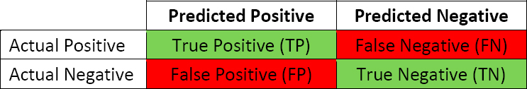
A variety of metrics are available to evaluate the performance of AI models completing classification tasks. The most common performance metrics are accuracy, precision, recall, and

F1. For a typical classification problem, it is of interest to measure the number of true positives (TP), the number of true negatives (TN), the number of false positives (FP), and the number of false negatives (FN) for each class. A common visual representation of the relationship between these quantities is the confusion matrix. Figure 50 shows the confusion matrix of true and predicted labels for an individual class.

For each class (UR or NUR), accuracy is the overall proportion of correctly predicted instances (both positive and negative). Accuracy is calculated as follows:

$Accuracy=\frac{{\displaystyle \sum TP+TN}}{{\displaystyle \sum TP+FP+FN+TN}}$

For each class, precision is the proportion of correctly predicted positive instances (i.e., true positives) with respect to all instances predicted as positive (i.e., true positives and FPs). Precision is calculated as follows:

$Precision=\frac{{\displaystyle \sum TP}}{{\displaystyle \sum TP+FP}}$

For each class, recall is the proportion of correctly predicted positive instances (i.e., true positives) with respect to all instances that were actually positive (i.e., true positives and FNs). Recall is calculated as follows:

$Recall=\frac{{\displaystyle \sum TP}}{{\displaystyle \sum TP+FN}}$

For each class, F1 is the harmonic mean of precision and recall. It provides a measure of overall performance that takes into account both precision and recall. F1 is calculated as follows:

$F_1=\frac{2}{\raisebox{1ex}{$1$}\!\left/ \!\raisebox{-1ex}{$Precision$}\right.+\raisebox{1ex}{$1$}\!\left/ \!\raisebox{-1ex}{$Recall$}\right.}$