Airport Greenhouse Gas Emissions Inventory: A Primer (2024)
Chapter: 3. Collect Data and Estimate Emission Sources
3. Collect Data and Estimate Emission Sources
After determining which emission sources to include in your airport’s GHG inventory based on the inventory boundaries, the next steps will be to determine the baseline inventory year, decide on the methods to use to calculate emissions, and identify the data that are needed to complete the calculations. You can then collect the data and estimate emissions for each source to complete your airport’s baseline GHG emissions inventory.
3.1 Establish a Baseline GHG Inventory
Airport operators must choose a base year, or a specific historical GHG inventory year that establishes a baseline against which progress toward emission reduction goals can be measured. You should select a base year for which you have reliable, verifiable, and representative emissions data. You should select a single year as your base year and you will need to decide whether to align with the calendar year or fiscal year. An annual average over consecutive (usually three) years may also be used for the base year. Using an annual average as a base year can smooth interannual variations in emissions.
It is common for an airport’s GHG emissions inventory to change over time. As an example, additional emission sources, such as Scope 3 sources, may be added or methods for estimating emissions may change as better data become available. In anticipation of these changes, it is best practice to develop a policy that stipulates when to recalculate the base year to incorporate changes. Your airport’s baseline emissions recalculation policy should include a quantitative or qualitative “significance threshold” that triggers historical emissions recalculations, such as changes to data, inventory boundaries, calculation methods, or other relevance factors. For example:
- Structural changes that would have a significant impact on the airport’s baseline emissions related to transfers of ownership, such as mergers, acquisitions, divestments, outsourcing, or insourcing of emissions-generating activities.
- Changes or improvements in calculation methods, emission factors, or activity data.
- Discoveries of significant errors.
Currently, there is no industry-wide standard for a significance threshold. When establishing your baseline inventory, you should determine your own quantitative or qualitative thresholds for triggering historical emissions recalculations and assess the need for recalculations for each subsequent inventory year.
3.2 Determine Inventory Methods
There are numerous resources available to assist you with identifying and applying GHG calculation methods. Guidance documents such as the Intergovernmental Panel on Climate Change (IPCC) 2006 Guidelines for National Greenhouse Gas Inventories provide methods for calculating emissions, while programs such as U.S. Environmental Protection Agency’s (EPA) Center for Corporate Climate Leadership provide emission factor sets and simple calculators. Organizations such as Airports Council International (ACI) provide tools such as the Airport Carbon and Emissions Reporting Tool (ACERT), a Microsoft Excel-based GHG inventory tool, and numerous companies provide commercially available GHG accounting software and services. Table 9-2 provides a summary of available resources.
When selecting methods—either to develop your own calculators or to apply publicly or commercially available tools and software—it is best practice to use equations and emission factors from reputable, publicly available sources, such as those provided by federal agencies or the IPCC.
3.3 Collect GHG Inventory Data
The quality of a GHG emissions inventory depends on the quality of the data used to produce it. Establishing and recording data collection procedures will help ensure that high-quality activity data is collected consistently across inventory years. Best practices for data collection are to:
- Identify an “inventory coordinator” who will determine the data needed to prepare the inventory and work with data holders across the airport to compile it. Table 3-1 provides an initial list of key data needs.
- Identify and document the data and information systems that house needed data and the individuals that maintain those systems by name and title.
- Collect and archive original source data (e.g., invoices) so that all data points are transparent and traceable.
- Archive emails and incorporate screenshots from emails that contain inventory assumptions in estimation spreadsheets and/or inventory management plans (see Section 4. Monitor Progress Over Time).
- Ensure that boundary decisions are consistently applied across emission sources.
- Compare the current inventory year data to previous years’ data and trends. Investigate and document year-to-year changes that are inconsistent with historical trends.
Emissions calculated using granular, site-specific activity data are the most accurate method for calculating emissions. However, if activity data are unavailable, proxy data from similar activities or previous inventories or secondary data may be used to fill in gaps, as illustrated in Figure 3-1.
Table 3-1: Example Activity Data Types and Sources by Emission Source
| Emission Source | Activity Data Types | Where Activity Data May Be Found | |
| Scope 1 | Stationary fuel combustion | Fuel consumption by quantity and type of fuel* | Utility bills or meters managed by facility staff |
| Dollars spent on fuel by fuel type | Utility bills or invoices managed by procurement staff | ||
| Scope 2 | Purchased electricity | Electricity consumption* | Utility bills or meters managed by facility staff |
| Dollars spent on electricity | Utility bills or invoices managed by procurement staff | ||
| Scope 3 | Purchased goods and services | Dollars spent on purchased goods and services | Purchase orders and purchasing card transactions managed by procurement staff |
| Fuel- and energy-related activities (not included in Scopes 1 and 2) | Fuel consumption by quantity and type of fuel* | Utility bills or meters managed by facility staff | |
| Dollars spent on fuel by fuel type | Utility bills or invoices managed by procurement staff |
* Indicates preferred activity data for more accurate emissions calculations.
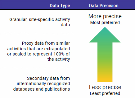
Table 3-1 shows examples of emission sources, the types of activity data needed to calculate emissions, and suggestions for where that activity data may be found in the airport operator’s organization for select emission sources.
If activity data is not available, airport operators may collect proxy data and use assumptions to calculate emissions. Table 3-2 shows examples of emission sources, proxy activity data, assumptions needed to calculate emissions, and where the proxy data may be found in the airport operator’s organization for select emission sources. Using proxy data may result in less accurate emissions calculations, so activity data should be used whenever available.
3.4 Estimate GHG Emissions
The calculations used to estimate GHG emissions are different for each emission source and vary in their complexity; however, they can be simplified into the following general equation:
Activity Data x GHG Emission Factor x Global Warming Potential = GHG Emissions
Wherein,
Activity Data is the data on the activities that generate emissions, such as 10 gallons of gasoline consumed by ground-support equipment (GSE). One gallon of gasoline contains 1 gigajoule (GJ) of energy, so 10 gallons of gasoline can also be expressed as 10 GJ.
GHG Emission Factors are factors that stipulate the emissions that result from a unit of activity data; as an example, 0.0096 kilograms (kg) of methane (CH4) per GJ.
Global Warming Potential (GWP) is a measure of how much energy the emissions of a GHG, such as CH4, will absorb in the atmosphere relative to an equivalent amount of carbon dioxide (CO2). GWPs allow inventory compilers to express emissions from all GHGs as though they were CO2. As an example, using the IPCC Fifth Assessment Report (AR5) 100-year time-horizon, CH4 has a GWP of 28 and nitrous oxide (N2O) has a GWP of 265; therefore, emitting 1 kg of CH4 is equivalent to emitting 28 kg of CO2 and 1 kg of N2O is equivalent to emitting 265 kg of CO2.
Table 3-2: Example Emission Sources by Proxy Data Types, Assumptions, and Sources
| Emission Source | Proxy Data Types | Proxy Data Assumptions | Where Proxy Data May Be Found | |
| Scope 1 | Stationary fuel combustion | Facility square footage | Fuel use intensity per square foot | Building records managed by facilities staff |
| Scope 2 | Purchased electricity | Facility square footage | Electricity use intensity per square foot | Building records managed by facilities staff |
| Scope 3 | Purchased goods and services | Dollars spent on purchased goods and services | Average emissions per dollar spent on purchased goods and services | Purchase orders and purchasing card transactions managed by procurement staff |
| Fuel- and energy-related activities (not included in Scopes 1 and 2) | Facility square footage | Fuel use intensity per square foot | Building records managed by facilities staff |
Please note that AR5 GWPs are used as the examples in this Primer, as those are the GWPs used by EPA in GHG inventory development at the time of publication. However, there are AR6 GWPs available, and airports can choose to use those GWPs if desired.
GHG Emissions are the emissions from all relevant GHGs that occur as a result of the activity. Emissions are expressed in units of carbon dioxide equivalent (CO2e).
The following section provides example equations to illustrate how the above calculation can be used to estimate emissions from various emission sources by scope.
Scope 1
3.5 Estimate Scope 1 Emissions
Scope 1 emissions are all direct GHG emissions from sources owned and/or controlled by the airport operator.
Scope 1 emission sources for airport operators may include:
- Vehicles/ground support equipment owned by the airport
- On-site waste management
- On-site wastewater management
- On-site power generation
- Firefighting exercises
- Boilers, furnaces
- De-icing substances
- Refrigerant losses
The following equations provide select examples for how to estimate emissions from these sources. Section 9.2. Resources for Emissions Calculations lists resources to help with Scope 1 emissions calculations.

Scope 1 Calculation Example: Emissions from Vehicles/Ground Support Equipment Owned
Fuel consumption quantity * fuel energy conversion factor * emission factor by gas * global warming potential by gas = emissions
| 1,000 gallons of diesel * 0.14 GJ/gallon of diesel = 136.73 GJ | |
| CO2: | 137 GJ * 74.10 kg CO2/GJ * 1 GWP = 10,131.62 kg CO2e |
| CH4: | 137 GJ * 0.0018 kg CH4/GJ * 28 GWP = 6.89 kg CO2e |
| N2O: | 137 GJ * 0.0012 kg N2O/GJ * 265 GWP = 42.03 kg CO2e |
| 10,131.62 kg CO2e + 6.89 kg CO2e + 42.03 kg CO2e = 10,180.55 kg CO2e | |
| 10,180.55 kg CO2e * (1 metric ton (MT))/1,000 kg) = 10.18 MT CO2e |
Scope 2
3.6 Estimate Scope 2 Emissions
Scope 2 emissions are all indirect GHG emissions associated with the generation of purchased electricity, steam, heat, or cooling consumed by the airport operator. These emissions physically occur at the facility where the electricity, steam, heating, or cooling is generated.
Scope 2 emissions for airport operators may include:
- Off-site electricity and steam purchased for heating, cooling, lighting, equipment operation and other purposes.
Scope 2 emissions from electricity consumption should, at a minimum, be calculated using location-based methods. Location-based electricity emissions reflect the average electricity emissions of the area where the airport is located and are typically calculated using emission factors supplied by EPA’s Emissions & Generation Resource Integrated Database (eGRID).
It is best practice for airport operators to also estimate market-based Scope 2 emissions. Market-based electricity emissions reflect the electricity emissions from sources an airport has purposely chosen, such as emissions from the utility from which the airport purchases electricity. Emission reductions from contractual instruments, such as the purchase of renewable energy certificates, are incorporated into market-based electricity emissions calculations.
See Section 10.2. Resources for Emissions Calculations for resources to help with Scope 2 emissions calculations.

Scope 2 Calculation Example: Location-Based Purchased Electricity Consumption
Electricity purchase quantity * electricity emission factor by gas * global warming potential by gas = emissions
| CO2: | 1,000,000 kilowatt hours (kWh) * 0.11 kg CO2/kWh * 1 GWP = 105,724.00 kg |
| CO2e: | 1,000,000 kWh * 0.11 kg CO2/kWh * 1 GWP = 105,724.00 kg CO2e |
| CH4: | 1,000,000 kWh * 0.000010 kg CH4/kWh * 28 GWP = 10.00 kg CO2e |
| N2O: | 1,000,000 kWh * 0.0000010 kg N2O/kWh * 265 GWP = 1.00 kg CO2e |
| 105,724.00 kg CO2e + 10.00 kg CO2e + 1.00 kg CO2e = 105,735.00 kg CO2e | |
| 105,735.00 kg CO2e * (1 MT/1,000 kg) = 105.74 MT CO2e |
This example calculation uses location-based electricity emissions for the NYUP eGRID region.
Scope 3
3.7 Estimate Scope 3 Emissions
Scope 3 accounts for all remaining indirect GHG emissions associated with an airport operator’s upstream and downstream activities. Scope 3 emissions occur as a result of operations or activities owned and/or controlled by entities other than the airport operator.
The GHG Value Chain (Scope 3) Standard includes 15 Scope 3 emission source categories. Table 3-3 presents the 15 Scope 3 categories and likely airport operator emission sources.
Including Scope 3 Emissions
It is currently optional to include Scope 3 emissions in GHG inventories under the GHG Corporate Standard. However, there is a growing expectation among stakeholders that organizations include Scope 3 emissions, as these emissions often make up the largest share of an organization’s emissions.

Table 3-3: Airport Scope 3 Emission Sources
| Emission Source Category | Example Airport Emission Sources | |
|---|---|---|
| 1 | Purchased Goods and Services |
|
| 2 | Capital Goods |
|
| 3 | Fuel- and Energy-Related Activities (Not Included in Scopes 1 and 2) |
|
| 4 | Upstream Transportation and Distribution |
|
| 5 | Waste Generated in Operations |
|
| 6 | Business Travel |
|
| 7 | Employee Commuting |
|
| 8 | Upstream Leased Assets |
|
| 9 | Downstream Transportation and Distribution |
|
| 10 | Processing of Sold Products |
|
| 11 | Use of Sold Products and Provided Services |
|
| 12 | End-of-Life Treatment of Sold Products |
|
| 13 | Downstream Leased Assets |
|
| 14 | Franchises |
|
| 15 | Investments |
|
A comprehensive GHG inventory includes all relevant Scope 3 emission sources. A Scope 3 screening will help you identify which Scope 3 categories are relevant to your airport by evaluating each Scope 3 source against the relevancy criteria presented in Table 3-4. You may benefit from reviewing the relevancy criteria with your stakeholder group to determine if some criteria should be weighted more heavily than others. As an example, is it important to invest the most effort in estimating large emission sources? If so, emissions related to the consumption of aviation fuel, such as emissions from aircraft LTO cycles and CCD under (Category 11: Use of Sold Products and Services) are likely to be relevant. Alternatively, are emissions that your airport can most easily reduce more important? What about emissions that most affect your airport’s risk exposure? Should all criteria be weighted equally? Questions such as these will be important to consider with your stakeholder group to help decide on relevant Scope 3 emission sources.
Once you have determined which Scope 3 emission sources are relevant, you can focus your resources on calculating emissions from those sources with greater accuracy and reducing those emissions.
See Section 9.2. Resources for Emissions Calculations for resources to help with Scope 3 emissions calculations.
Table 3-4: Scope 3 Relevancy Criteria
| Scope 3 Relevancy Criteria | Criteria Definition |
|---|---|
| Occurring | Emissions are known to occur from a specific source. |
| Size | Emission source contributes significantly to your airport’s total anticipated Scope 3 emissions. |
| Influence | There are potential emission reductions that could be undertaken or influenced by your airport. |
| Risk | Emission source contributes to your airport’s risk exposure (e.g., climate change related risks such as financial, regulatory, supply chain, product and technology, compliance/litigation, and reputational risks). |
| Stakeholders | Emission source is deemed critical by your airport’s key stakeholders (e.g., customers, suppliers, or civil society). |
| Outsourcing | Emission source is an outsourced activity previously performed in-house or activity outsourced by your airport that is typically performed in-house by other airports. |
| Sector Guidance | Emission source as been identified as significant by sector-specific guidance. |
| Spending or Revenue Analysis | Emission source is an area that requires a high level of spending or generates a high level of revenue for your airport. |
Scope 3 Calculation Example: Aircraft LTO Cycle
Total fuel consumed in LTO cycle by aircraft type * fuel emission factor by gas * global warming potential by gas = emissions
| CO2: | 263 gallons of kerosene consumed during Boeing 757 LTO cycle * 9.75 kg CO2/gallon kerosene * 1 GWP = 2,564.25 kg CO2e |
| CH4: | 263 gallons of kerosene consumed during Boeing 757 LTO cycle * 0 kg CH4/gallon kerosene * 28 GWP = 0 kg CO2e |
| N2O: | 263 gallons of kerosene consumed during Boeing 757 LTO cycle * 0.00030 kg N2O/gallon kerosene * 265 GWP = 20.91 kg CO2e |
| 2,564.25 kg CO2e + 0 kg CO2e + 20.91 kg CO2e = 2,585.16 kg CO2e | |
| 2,585.16 kg CO2e * (1 MT/1,000 kg) = 2.59 MT CO2e |
Scope 3 Calculation Example: APU
Fuel consumed by APU * fuel emission factor by gas * global warming potential by gas = emissions
| APU running for 60 minutes * 0.59 gallons kerosene/minute APU is running for a Boeing 757 = 35.40 gallons kerosene | |
| CO2: | 35.40 gallons kerosene * 9.75 kg CO2/gallon Jet A * 1 GWP = 345.15 kg CO2e |
| CH4: | 35.40 gallons kerosene * 0.00 kg CH4/gallon Jet A * 28 GWP = 0.00 kg CO2e |
| N2O: | 35.40 gallons kerosene * 0.00030 kg N2O/gallon Jet A * 265 GWP = 2.81 kg CO2e |
| 345.15 kg CO2e + 0.00 kg CO2e + 2.81 kg CO2e = 347.96 kg CO2e | |
| 347.96 kg CO2e * (1 MT/1,000 kg) = 0.35 MT CO2e |


