Evaluation of Post-Consumer Recycled Plastics in Asphalt Mixtures via the Dry Process (2025)
Chapter: 4 Results and Findings
CHAPTER 4
Results and Findings
4.1 Experiment 1: Characterization and Selection of PCR Plastics
This section provides the physical, thermal, and chemical characterization results of 12 PCR plastics in Experiment 1, as well as the selection of 5 PCR plastics for further evaluation in Experiment 5 to determine the impact of different PCR plastics on the performance properties of asphalt mixtures when added via the dry process.
4.1.1 Physical Characterization
Figure 17 presents the MFI results at 190°C (374°F) with a 2.16 kg load. As shown, the 12 PCR plastic samples cover a wide range of MFI values, varying from 0 to 13.6 g/10 min., indicating distinctly different flow properties. Sample #4 had the highest MFI, followed by Samples #12, #9, and #1, respectively, while the rest of the samples had comparably low MFI values. Based on two preliminary MFI limits, the 12 PCR plastics can be separated into three groups with different flow properties:
- Group 1: Samples #4 and #12 had MFIs over 5 g/10 min., indicating low flow resistance (i.e., low viscosity).
- Group 2: Samples #1 and #9 had MFIs between 2 g/10 min. and 5 g/10 min., indicating intermediate viscosity.
- Group 3: Samples #2, #3, #5, #6, #7, #8, #10, and #11 had MFIs below 2 g/10 min., indicating high viscosity.
Additional MFI testing was also conducted at 190°C (374°F) with a 10 kg load, and the test results yielded the same grouping of the 12 PCR plastic samples as the 2.16 kg load.
Table 14 summarizes the results for molecular weights measured in the gel permeation chromatography (GPC). Samples #11 and #12 were excluded from GPC testing because of the high number of insoluble materials detected during sample preparation. Mn is the number-average molecular weight, and it influences the thermodynamic properties of polymers (Dawkins, 1979). Mw is the weight-average molecular weight, and it is sensitive to large molecules, influencing the melt viscosity of polymers (Aguilar-Vega, 2013). Mz is the z-average molecular weight, and it is sensitive to larger molecules, influencing the viscoelastic properties or melt elasticity of polymers (Aguilar-Vega, 2013). The ratio of Mw to Mn is used to calculate a polymer’s polydispersity index (PDI), indicating the material’s range of molecular mass (Moraes and Bahia, 2015). The broader the molecular weight distribution, the larger the PDI. Mp is the molecular weight at the peak of the GPC molecular-weight-distribution curve.

Based on the GPC results for Mw, which is related to the melt viscosity of polymers and thus can influence the processing of the recycled samples, the tested PCR plastics can be separated into three groups with different ranges of molecular weights:
- Group 1: Samples #1 and #9 had an Mw of 94.1 × 10³ daltons and 93.0 × 10³ daltons, respectively, presenting the lowest molecular weights.
- Group 2: Samples #2, #4, #5, and #8 each had an Mw between 112.1 and 120.7 × 10³ daltons, presenting intermediate molecular weights.
- Group 3: Samples #3, #6, #7, and #10 each had an Mw between 122.1 and 137.9 × 10³ daltons, presenting the highest molecular weights.
As Figure 18 indicates, there is a fair inverse relationship between MFI and Mw for the PCR plastic samples (R2 = 0.55). However, this correlation should be interpreted with caution as it is only appropriate for comparing MFI and Mw of the same polymer types (LDPE, HDPE, PP, etc.) due to the impact of branching and chemistry on MFI (Bremner and Rudin, 1990; Bremner et al., 2003). For the PCR plastic samples, a poor inverse correlation was observed between MFI and Mn (R2 = 0.09), MFI and Mz (R2 = 0.03), and MFI and Mp (R2 = 0.43).
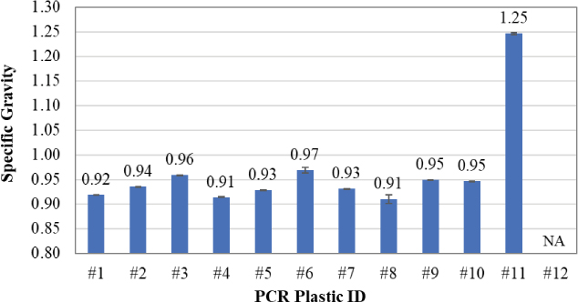
Figure 19 presents the specific gravity results. As shown, nearly all the PCR plastic samples—except Samples #11 and #12—had similar specific gravity values within the range of 0.91 to 0.97, slightly lower than the specific gravity of the asphalt binder. Sample #11 had a significantly higher specific gravity of 1.25 due to the presence of CaCO3 in the composition. The specific gravity of Sample #12 is reported as “NA” (not available) because the shape irregularities of the material interfered with an accurate density measurement due to the presence of air voids. Except for Sample #11, there was no noticeable distinction among the selected PCR plastic samples in terms of specific gravity.
Table 14. GPC molecular weights of PCR plastic samples.
| PCR Plastic Sample ID | Mn x 103 (daltons) | Mw x 103 (daltons) | Mz x 103 (daltons) | Mp x 103 (daltons) | Mw/Mn x 103 (daltons) |
|---|---|---|---|---|---|
| #1 | 23.8 | 94.1 | 270.4 | 64.5 | 3.9 |
| #2 | 20.9 | 117.8 | 491.2 | 72.3 | 5.6 |
| #3 | 15.6 | 124.8 | 751.2 | 38.7 | 8.0 |
| #4 | 22.4 | 114.0 | 316.8 | 82.0 | 5.1 |
| #5 | 26.2 | 120.7 | 407.6 | 76.9 | 4.6 |
| #6 | 17.3 | 137.9 | 655.1 | 78.6 | 8.0 |
| #7 | 21.1 | 122.1 | 479.7 | 75.4 | 5.8 |
| #8 | 25.6 | 112.1 | 379.3 | 72.1 | 4.4 |
| #9 | 17.6 | 93.0 | 434.1 | 44.7 | 5.3 |
| #10 | 19.9 | 132.4 | 541.6 | 75.6 | 6.7 |

Figure 20 summarizes the pellet count and average pellet weight results. As discussed previously, Samples #6, #8, #11, and #12 are in non-pellet form; thus, they were excluded from the particle size analysis. Among the samples tested, the pellet count varied from 19 to 76 pellets/g, and the average pellet weight varied from 0.013 to 0.060 g/pellet.
Solubility testing was performed to determine the ability of the 12 PCR plastic samples to dissolve in 1, 2, 4 trichlorobenzene (TCB) as a function of temperature (from 20°C to 170°C) and concentration of the PCR plastics [1%, 2.5%, 5%, and 10% weight per volume (w/v)]. For sample preparation, the PCR plastics were weighed in clear glass vials and then the solvent was added, and the vials were sealed with septum closures. A control vial containing only TCB was used to monitor the solvent temperature throughout the heating process. Table 15 summarizes the observed stages of the PCR plastic samples in the solubility experiment for concentrations of 1% and 5% w/v and for temperature values of 20°C to 35°C and 170°C.
The 12 PCR plastic samples were insoluble in TCB at low temperatures (20°C–35°C), regardless of the concentration (i.e., 1% and 5% w/v). With the exception of Sample #6—which was insoluble at both low and high temperatures—as the temperature increased to 170°C, the state of the plastic samples in TCB changed from insoluble (no visible change was observed in the PCR plastic pellets or strands) to swollen (the PCR plastic pellets or strands increased in size while lightening in color), partially soluble, largely soluble, or soluble (the PCR plastic pellets
Note: NA = not available.

Note: N/A = not applicable.
Table 15. Observed stages of the PCR plastic samples in the solubility experiment.
| PCR Plastic Sample ID | 1% PCR in TCB (w/v) | 5% PCR in TCB (w/v) | ||
|---|---|---|---|---|
| 20ºC–35ºC | 170ºC | 20ºC–35ºC | 170ºC | |
| #1 | Insoluble | Partially soluble | Insoluble | Partially soluble |
| #2 | Insoluble | Swollen | Insoluble | Swollen |
| #3 | Insoluble | Swollen Partially soluble | Insoluble | Swollen Partially soluble |
| #4 | Insoluble | Swollen Partially soluble | Insoluble | Swollen Partially soluble |
| #5 | Insoluble | Swollen | Insoluble | Swollen |
| #6 | Insoluble | Insoluble | Insoluble | Insoluble |
| #7 | Insoluble | Swollen | Insoluble | Swollen |
| #8 | Insoluble | Largely soluble | Insoluble | Largely soluble |
| #9 | Insoluble | Soluble | Insoluble | Soluble |
| #10 | Insoluble | Soluble | Insoluble | Soluble |
| #11 | Insoluble | Partially soluble | Insoluble | Swollen Partially soluble |
| #12 | Insoluble | Soluble | Insoluble | Soluble |
or strands were fully dissolved), while some samples became both swollen and partially soluble. At 170°C, Samples #9, #10, and #11 were soluble in TCB at the two evaluated concentrations (1% and 5% w/v).
4.1.2 Thermal Characterization
Table 16 summarizes the thermal properties of crystallization and melting measured in the DSC. From the cooling curves, the temperatures of each peak of crystallization (Tc1, Tc2, Tc3) and the enthalpy of crystallization (ΔHcrystallization) were measured. From the melting curves, the temperatures of each melting peak (Tm1, Tm2, Tm3) and the enthalpy of melting (ΔHmelting) were measured. Due to the presence of filler in the PCR plastic samples, it was not possible to determine the glass transition temperature (Tg) of the samples within the DSC curves. The percentage of crystallinity was not calculated due to the presence of multiple resins within the samples.
From the crystallization curves of Samples #1, #5, #11, and #12, three exothermic peaks (Tc1, Tc2, Tc3) were observed. For Samples #2, #7, #9, and #10, two exothermic peaks (Tc1, Tc2) were observed. Samples #3, #4, #6, and #8 presented only one exothermic peak (Tc1). From the melting curves, Sample #7 presented three endothermic peaks (Tm1, Tm2, Tm3), while Sample #12 presented only one endothermic peak (Tm1). All other samples presented two endothermic peaks (Tm1, Tm2). Based on the initial crystallization temperatures (Tc1), the 12 PCR plastic samples can be separated into three groups with different ranges of cold crystallization exotherms:
- Group 1: Samples #1, #2, #5, #7, #8, and #10 had crystallization onset temperatures between 109°C and 113°C, presenting the lowest cold crystallization exotherms.
- Group 2: Samples #3, #4, #6, #9, and #12 had crystallization onset temperatures between 116°C and 123°C, presenting intermediate cold crystallization exotherms.
- Group 3: Sample #11 had a crystallization onset temperature of 202°C, presenting the highest cold crystallization exotherm.
A similar grouping was observed when considering the initial melting temperatures (Tm1) of the 12 PCR plastic samples, indicated in the following list. The only change in grouping occurred for Sample #12, which was included among the Group 1 samples for Tm1 and Group 2 samples for Tc1:
- Group 1: Samples #1, #2, #5, #7, #8, #10, and #12 had the lowest melting onset temperatures, between 121°C and 130°C. This range of melting temperature below 130°C indicates the presence of PE in the PCR plastic samples.
- Group 2: Samples #3, #4, #6, and #9 had intermediate melting onset temperatures, between 159°C and 164°C.
- Group 3: Sample #11 had the highest melting onset temperature at 235°C.
Table 16. DSC crystallization and melting parameters.
| PCR Plastic Sample ID | Cooling Ramp (Crystallization) | Heating Ramp (Melting) | ||||||
|---|---|---|---|---|---|---|---|---|
| Tc1 (°C) |
Tc2 (°C) |
Tc3 (°C) |
ΔHcrystallization (J/g) |
Tm1 (°C) |
Tm2 (°C) |
Tm3 (°C) |
ΔHmelting (J/g) |
|
| #1 | 110 | 98 | 62 | 138 | 122 | 110 | NA | 142 |
| #2 | 113 | 99 | NA | 150 | 124 | 111 | NA | 142 |
| #3 | 120 | NA | NA | 206 | 163 | 131 | NA | 214 |
| #4 | 123 | NA | NA | 103 | 159 | 126 | NA | 109 |
| #5 | 109 | 98 | 63 | 143 | 121 | 109 | NA | 142 |
| #6 | 116 | NA | NA | 145 | 160 | 125 | NA | 149 |
| #7 | 112 | 98 | NA | 145 | 123 | 109 | 161 | 152 |
| #8 | 113 | NA | NA | 135 | 122 | 113 | NA | 132 |
| #9 | 119 | 102 | NA | 187 | 164 | 130 | NA | 194 |
| #10 | 113 | 97 | NA | 144 | 124 | 110 | NA | 149 |
| #11 | 202 | 201 | 113 | 59 | 235 | 164 | NA | 61 |
| #12 | 119 | 98 | 62 | 188 | 130 | NA | NA | 184 |
Note: NA = not available.

Figure 21 presents the ash content results. As shown, Sample #11 has the highest ash content of 6.5%, followed by Samples #6 (4.6%), #8 (3.9%), and #10 (2.6%); the rest of the samples have relatively low ash contents (below 1.5%). Table 17 presents the plastic additive contents detected through the TGA. In summary, all the samples contain common additives, including inorganic fillers [such as CaCO3, silica (SiO2), and titanium dioxide (TiO2)], slip agents [such as calcium stearate (CaSt) and zinc stearate (ZnSt)], antioxidants (such as Irganox 1425), scavengers (such as DHT-4A), and other additives (such as NA-11 nucleating agent).
4.1.3 Chemical Characterization
The VOC analysis was conducted through direct headspace-gas chromatography (headspace-GC). In headspace-GC, a sample is volatilized and carried by an inert gas through a coated glass capillary column, where a stationary phase is bonded to the interior of the column. The time it takes a specific compound to pass through the column to a detector is called retention time and
Table 17. Additive contents detected through TGA.
| PCR Plastic Sample ID | Additive Content (ppm) | ||||||||||||
|---|---|---|---|---|---|---|---|---|---|---|---|---|---|
| Zn | Ti | Si | S | P | Na | Mo | Mg | Ca | Ba | Al | Cl | Potential Additives | |
| #1 | 400 | 24.4 | 224 | 14.9 | 62.9 | 94.8 | <5 | 66.3 | 377 | 6.2 | 106 | 164 | DHT-4A, CaCO3, CaSt, Irganox 1425, SiO2, TiO2, ZnSt |
| #2 | 161 | 484 | 1,140 | 67.9 | 51.1 | 145 | <5 | 853 | 3,200 | 59.1 | 559 | 425 | DHT-4A, CaCO3, CaSt, Irganox 1425, SiO2, TiO2, ZnSt |
| #3 | 19.8 | 3,730 | 354 | 73.2 | 25 | 55.3 | <5 | 74.1 | 1,520 | 115 | 142 | 110 | DHT-4A, CaCO3, CaSt, Irganox 1425, SiO2, TiO2 |
| #4 | 30.1 | 2,200 | 280 | 65.6 | 46 | 94.6 | <5 | 209 | 1,570 | 78.2 | 130 | 71.3 | DHT-4A, CaCO3, CaSt, Irganox 1425, SiO2, TiO2 |
| #5 | 39.9 | 2.65 | 374 | <5 | 32.6 | 50.1 | <5 | 309 | 5,020 | <5 | 41.7 | 11.3 | DHT-4A, CaCO3, CaSt, Irganox 1425, SiO2, TiO2 |
| #6 | 87.9 | 970 | 1,100 | 125 | 36.7 | 237 | <5 | 452 | 12,900 | 185 | 413 | 111 | DHT-4A, CaCO3, CaSt, Irganox 1425, SiO2, TiO2, ZnSt |
| #7 | 96.7 | 202 | 1,540 | 82 | 36 | 203 | <5 | 348 | 2,900 | 119 | 252 | 351 | DHT-4A, CaCO3, CaSt, Irganox 1425, SiO2, TiO2, ZnSt |
| #8 | 48.6 | 1,260 | 3,280 | 35 | 60.5 | 388 | <5 | 1,460 | 8,810 | 15.7 | 375 | 67.7 | DHT-4A, CaCO3, CaSt, Irganox 1425, SiO2, TiO2 |
| #9 | 53 | 1,460 | 484 | 106 | 33.4 | 216 | <5 | 196 | 1,450 | 129 | 178 | 307 | DHT-4A, CaCO3, CaSt, Irganox 1425, SiO2, TiO2, talcum (talc) |
| #10 | 86.9 | 3,800 | 1,890 | 121 | 44.3 | 325 | <5 | 601 | 2,190 | 191 | 492 | 833 | DHT-4A, CaCO3, CaSt, Irganox 1425, SiO2, TiO2, talc, ZnSt |
| #11 | <5 | 370 | 679 | 255 | 67.3 | 839 | <5 | 878 | 14,000 | 6.3 | 872 | 355 | DHT-4A, CaCO3, CaSt, Irganox 1425, SiO2, TiO2, talc |
| #12 | 51.2 | 334 | 421 | 186 | 39.3 | 147 | <5 | 72.3 | 1,990 | 58.7 | 179 | 126 | CaCO3, CaSt, DHT-4A, NA-11, talc, TiO2 |
can be used for the identification of compounds when compared to a reference. This headspace-GC method has been successfully used for the analysis of VOCs released during the preparation of asphalt mixtures in a laboratory environment (Stroup-Gardiner and Lange, 2005; Osborn, 2015). The Agilent MassHunter Unknowns Analysis was used as the preprocessing tool for the headspace-GC/mass spectrometer (MS) data, which consists of an integrated set of procedures for first extracting pure component spectra and related information from complex chromatograms, then using this information to determine whether the component can be identified as one of the compounds represented in a reference library (Mallard and Reed, 1997).
All samples were analyzed by an Agilent 7890/5975 gas chromatograph/MS equipped with a Gerstel MPS2 Robotic autosampler using headspace. The gas chromatograph had a 30 m × 0.25 mm × 1.0 μm RTX-Volatiles column equipped. The inlet was equipped with a 4 mm single gooseneck liner, Merlin 23-gauge septa, and operated in split mode with a 2:1 split ratio and an initial pressure of 14.115 psi. The column was operated in a ramped flow program with an initial flow of 1.3 mL/min. for 10 minutes, then ramped at 0.25 to 1.75 mL/min. The oven program had an initial temperature of 35°C for 3 minutes, then ramped 12°C/min. to 260°C and held for 10 minutes. The MS was operated in the full scan acquisition mode with the bfb.u tune setting. The bfb.u tune setting is designed by the manufacturer to obtain a mass spectrum with reproducible ion ratios suitable for library screening for volatile compounds according to the EPA methods. The scan range was from 35 to 400 m/z. The autosampler was equipped with a 2.5 mL headspace syringe that was heated to 150°C. Samples were incubated at 165°C for 60 minutes, with agitation set to 500 rpm on a 90 seconds “on” and 30 seconds “off” cycle. A 1,000 μL aliquot of the vapor phase of the sample was taken for analysis by the autosampler and then injected at 200 μL/s. After injection, the syringe was flushed for 120 seconds with helium.
Sample vials were prepared by weighing 3 mm glass beads into a headspace vial at 15 g for each of the 12 samples. Due to availability, the PCR material was prepared in two separate batches using the same sample procedure. PCR plastic samples were massed on clean weigh boats and then transferred to the top of the prepared sample vials (Figure 22). Sample weights were approximately 0.5 g. A toluene-d8 internal standard was added using a 10 μL syringe to deliver 5 μL of the 2,500 μg/mL solution, resulting in 12.5 μg of toluene-d8 added.
Figure 23 presents the total VOC results of the 12 PCR plastic samples obtained from the headspace-GC/MS analysis. Overall, the plastic samples showed different odor/fume potentials.

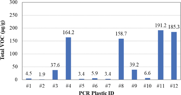
Samples #1, #2, #5, #6, #7, and #10 had the lowest total VOC values, ranging between 1.9 and 6.6 μg/g. Samples #3 and #9 had similar values of total VOC (37.6 and 39.2 μg/g, respectively). Samples #4, #8, #11, and #12 had the highest total VOC values, ranging between 158.7 and 191.2 μg/g. The headspace-GC/MS analysis also identified the presence of benzene (a very hazardous compound) at a concentration of approximately 1.9 μg/g in Sample #11. Figure 24 through Figure 35 present the chromatograms of individual PCR plastic samples.
Table 18 summarizes the FTIR composition analysis results. Based on the surface scans using attenuated total reflectance, PE was detected in every PCR plastic sample except for Samples #10 and #11. PP was detected in Samples #4 and #9, while PET was detected in Samples #10 and #11. The surface scans also detected the presence of glycerol monostearate (GMS) in Samples #4 and #7, which indicates that these samples may be sourced from food packaging materials. The transmission scans (using pressed films) detected the presence of polyamides in Samples #2, #7, and #10, suggesting these samples are sourced from multilayer packaging materials. Polyester or polyamide is often used with PE as a component in multilayer food packaging. The transmission scans also detected talcum, or talc, and CaCO3 in all the samples except Samples #2, #10, and #11, but surface scans detected CaCO3 in Sample #2. Figure 36 through Figure 47 present the FTIR surface spectrum of individual PCR plastic samples.
4.1.4 Selection of Five PCR Plastics for Experiment 5
The test results presented in this section were evaluated against a set of criteria to select five PCR plastics for further evaluation in Experiment 5. All selection criteria and the resultant outcomes are provided as follows (continued after figures):
- Select plastic samples with low odor and fume potential due to safety considerations. Based on the VOC results in Figure 23, this selection criterion eliminates Samples #4, #8, #11, and #12.
- Select plastic samples containing PE or PP, or both, because PE and PP together account for the largest proportion of plastic types in municipal solid waste, and they have relatively low melting temperatures within typical production temperatures for asphalt mixtures. Based on the FTIR results in Table 18, this selection criterion eliminates Samples #10 and #11.
- Prioritize plastic samples with different flow properties, based on the MFI results in Figure 17.
- Prioritize plastic samples with different molecular weights, based on the GPC results in Table 14.

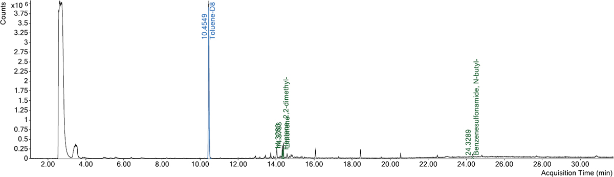

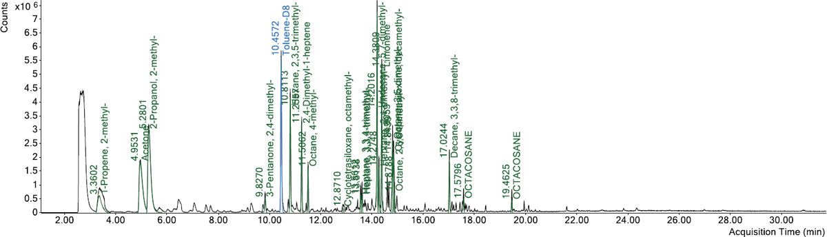


Table 18. FTIR composition analysis results.
| PCR Plastic Sample ID | PE | PP | GMS | Slip Agents | PET | Clay | Talc | CaCO3 | Amide I/II |
|---|---|---|---|---|---|---|---|---|---|
| #1 | X | O | O | O | |||||
| #2 | X | X | X | O | |||||
| #3 | X | O | O | O | |||||
| #4 | X | X/O | X | O | X/O | ||||
| #5 | X | O | O | X/O | |||||
| #6 | X | O | O | O | |||||
| #7 | X | O | X | X | O | O | O | ||
| #8 | X | O | O | ||||||
| #9 | X | X/O | O | O | |||||
| #10 | X | X | O | ||||||
| #11 | X | ||||||||
| #12 | X | O | O |
Note: Functionality detected via surface scans or transmission scans (designated with X and O, respectively).
- Prioritize plastic samples used in recent field projects.
- Sample #1 was used in the NCAT/Minnesota Road Research Facility (MnROAD) Additive Group experiments and a field project in Missouri.
- Sample #2 was used in the Wisconsin field project tested in Experiment 2.
- Sample #5 was used in the Ohio field project tested in Experiment 2.
Based on these criteria, Samples #1, #2, #5, #7, and #9 were selected for further evaluation in Experiment 5, which focused on mixture performance testing of laboratory-prepared RPM asphalt mixtures with different PCR plastics as well as rheological and chemical characterization of extracted RPM asphalt binders.
4.2 Experiment 2: Laboratory Characterization of Plant-Produced RPM versus Control Asphalt Mixtures and Extracted Binders
This section presents the laboratory test results of plant-produced RPM versus control asphalt mixtures and their extracted binders from two field projects in Experiment 2. The focus of the comparison was to determine how the RPM mixture/binder performed compared to the control counterpart.
4.2.1 Mixture Test Results
For all mixture tests except the HWTT, the results are presented using column charts, where the columns represent the average index test parameters of each mixture, and the error bars represent plus and minus one standard deviation from the average. In addition, a statistical t-test at a significance level of 0.05 was performed to determine if statistical differences existed between the control and RPM mixtures in terms of the index test parameters.
Workability
Figure 48 shows the DWT results at 107°C (225°F), 121°C (250°F), and 135°C (275°F). For both projects, the RPM mixtures consistently exhibited lower average DWT values than the corresponding control mixtures at three testing temperatures, indicating reduced mixture workability. This reduction in workability was likely caused by the increased stiffness of the RPM mixtures compared to the control mixtures (Angelone et al., 2016; Diefenderfer and McGhee, 2015). For both control and RPM mixtures, the average DWT values increased with the testing temperature,


which indicates improved mixture workability due to the reduced binder viscosity at higher testing temperatures. However, the statistical t-test revealed that no statistical difference exists between the control and RPM mixtures in terms of DWT results for both projects except for the Wisconsin project at 121°C (250°F).
Stiffness and Aging Resistance
Figure 49 and Figure 50 present the |E*| master curves of RH and CA specimens for the control versus RPM mixtures from the two field projects. Although the control and RPM mixtures had comparable |E*| values at low temperatures and high frequencies (right-hand side of the master curve) at both aging conditions, their |E*| values differed at high temperatures and low frequencies (left-hand side of the master curve). For both projects, the RPM mixtures had notably higher |E*| and lower phase angles at high temperatures and low frequencies than the control mixtures, indicating that adding PCR plastics via the dry process increased the mixture’s stiffness, which is consistent with other studies (Angelone et al., 2016; López et al., 2018). Additionally, the |E*| results show that the stiffness of both control and RPM mixtures increased after critical aging, but the differences were not statistically significant in most cases (i.e., temperature-frequency combinations).

Figure 51 presents the Mixture Glover-Rowe (G-Rm) parameter results of the control versus RPM mixtures. For both field projects, the RPM mixture had considerably higher G-Rm than the control mixture, indicating increased brittleness and potentially higher susceptibility to block cracking. The ratio of the G-Rm of CA over the G-Rm of RH for the specimens was calculated to assess the aging susceptibility of the mixtures, and the results are summarized as follows: 1.71 for the Ohio control mixture versus 1.46 for the Ohio RPM mixture, and 1.75 for the Wisconsin control mixture versus 1.62 for the Wisconsin RPM mixture. These results indicate that adding PCR plastics via the dry process appeared to improve the aging resistance of asphalt mixtures.

Rutting Resistance
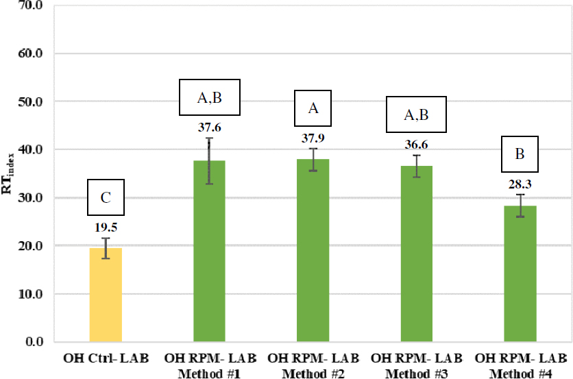
Figure 52 presents the rutting tolerance index (RTindex) results at 58°C (136°F). As shown, the RPM mixtures had consistently higher average RTindex values than the corresponding control mixtures, indicating improved rutting resistance. This improvement is attributed to the overall stiffening effect of adding recycled plastics (concluded from the |E*| master curves in Figure 49 and Figure 50), which consequently enhances the mixture’s resistance to high-temperature permanent deformation. The statistical t-test analysis demonstrated that a statistically significant difference exists between the RTindex results of the control versus RPM mixtures for both projects.
Figure 53 presents the HWTT rut depth curves at 46°C (115°F). For both projects, the RPM mixtures had considerably less rutting than the control mixtures in the HWTT, which indicates improved rutting resistance due to adding PCR plastics. This finding is consistent with the IDEAL-RT results shown in Figure 52. Furthermore, the RPM mixtures had no signs of stripping, whereas the control mixtures exhibited late stripping failures in the HWTT, as indicated by the stripping inflection point (SIP) results in Figure 53.


Moisture Susceptibility
Figure 54 shows the ITS results at both dry (unconditioned) and wet (moisture-conditioned) conditions. For both projects, the moisture-conditioned samples had a significantly lower ITS compared to the unconditioned samples for the control and RPM mixtures, indicating reduced ITS due to moisture conditioning and freezing-thaw cycles per AASHTO T 283. For both projects, the RPM mixtures that were either unconditioned or moisture-conditioned had higher ITS compared to the corresponding control mixtures, and the differences were statistically significant according to the t-test.
Figure 55 shows the corresponding TSR results of the control versus RPM mixtures. For both projects, each RPM mixture had a slightly higher TSR compared to the corresponding control mixture; however, the difference was less than the test’s repeatability range of 9.3% (Azari, 2010), and thus, it is not considered to be practically significant. Overall, the TSR results indicate that adding PCR plastics via the dry process did not have a significant impact on the moisture susceptibility of asphalt mixtures for both field projects.
Cracking Resistance
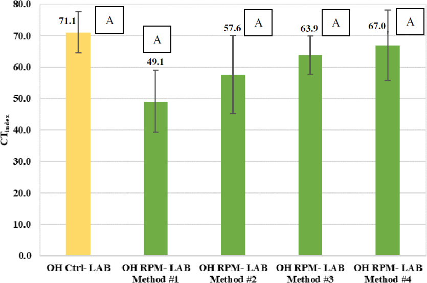
Figure 56 presents the IDEAL-CT results. The test was conducted on CA specimens that were further aged for 6 hours at 135°C (275°F) after reheating. For both field projects, the RPM mixture had a lower average cracking tolerance index (CTindex) than the corresponding control mixture, and the differences were statistically significant according to the t-test. This indicates that adding PCR plastics via the dry process had a detrimental effect on the intermediate-temperature cracking resistance of asphalt mixtures.


In addition to the CTindex comparisons, the IDEAL-CT interaction diagram (Figure 57) was used to explore the impact of adding PCR plastics on mixture toughness and brittleness. The diagram plots the average fracture energy (Gf), or mixture toughness, on the y-axis against the average l75/|m75| ratio (relative ductile-brittle behavior of the mixture) on the x-axis. Higher Gf and l75/|m75| values result in a higher CTindex. Thus, asphalt mixtures with a higher CTindex are located closer to the upper-right corner of the diagram (with higher Gf and l75/|m75|) compared to those with a lower CTindex. The interaction diagram also includes a series of CTindex contour curves, and the data points on each contour curve have the same CTindex but different Gf and l75/|m75| (Yin et al., 2023). As shown in Figure 57, adding PCR plastics via the dry process resulted in RPM mixtures with reduced Gf and l75/|m75| values (indicating reduced toughness and increased brittleness), which as a result moved the RPM mixtures toward the bottom-left corner of the interaction diagram compared to the control mixtures for both field projects.
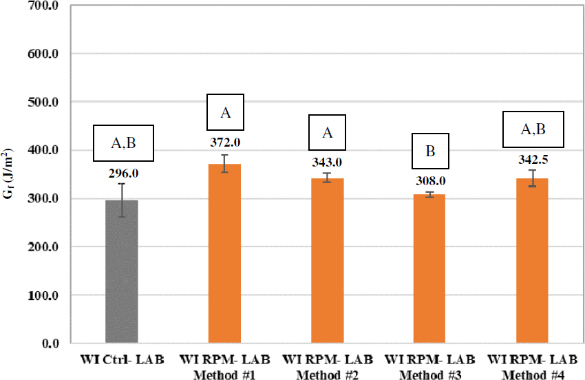
Figure 58 presents the DCT Gf results. The DCT test was also conducted on CA specimens to consider the impact of asphalt aging. The control and RPM mixtures from the Ohio project had statistically equivalent Gf results; thus, they are expected to have similar low-temperature cracking resistance. However, the RPM mixture from the Wisconsin project exhibited a different trend, with significantly higher Gf compared to the control mixture, indicating improved low-temperature cracking resistance attributed to the addition of PCR plastics via the dry process. This discrepancy could stem from the different sources of recycled plastics used in the two field projects. The DCT results were also analyzed using the fracture strain tolerance (FST) parameter recommended by Zhu et al. (2017) and Dave et al. (2021), and the results showed the same trend as the Gf results discussed previously.
Figure 59 presents the CF test results using the fatigue index parameter (Sapp). The test was conducted on CA specimens with additional loose mix aging for 6 hours at 135°C (275°F) after reheating. For both projects, the RPM mixture had a lower representative Sapp value compared to the control mixture, indicating reduced fatigue resistance due to adding PCR plastics via the dry process. This result likely occurred because adding PCR plastics increased the stiffness and brittleness of the mixtures, making them more susceptible to fatigue damage. As shown in Figure 60, the Sapp results are consistent with the CTindex results despite the distinctly different mechanisms of the CF test compared to the IDEAL-CT.
Figure 61 shows the C-versus-S curves of the control versus RPM mixtures. For both projects, the RPM mixture had less fatigue damage tolerance (as indicated by shorter C-versus-S curves) than the corresponding control mixture. Similar trends were observed for the predicted Nf-versus-strain results in Figure 62, where the control mixture showed significantly better fatigue resistance (as indicated by higher predicted Nf values over a wide range of strain levels)


than the dry-process RPM mixture for both projects. Overall, the CF test results indicate that adding PCR plastics via the dry process had a detrimental impact on the fatigue resistance of asphalt mixtures.
Surface Texture and Friction
Figure 63 presents the MPD results for the plant-produced control versus RPM mixtures from both projects. As shown in Figure 63, in all cases except for the Wisconsin control mixture, the MPD decreased after the first 50,000 polishing cycles and then plateaued after that. However, the MPD of the Wisconsin control mixture generally increased with additional polishing cycles, which might be attributed to the loss of fine particles during polishing and weathering. For both field projects, the RPM mixture had comparable MPD results to the control mixture throughout the polishing and weathering process, which implies that adding PCR plastics via the dry process had a negligible effect on the surface texture of asphalt mixtures.

Figure 64 presents the DFT40 results of the control versus RPM mixtures. As shown, the DFT40 of all four mixtures increased significantly after the first 50,000 polishing cycles, which is attributed to asphalt film wearing off from the mixture surface. After that, the DFT40 generally remained consistent in all cases except for the Ohio RPM mixture, which continued to decline with additional surface polishing and weathering. For the Ohio project, the control mixture had similar DFT40 results as the RPM mixture at the first and second measurements, but lower DFT40 results at the third and fourth measurements. Conversely, the control and RPM mixtures from the Wisconsin project had similar DFT40 results at all four measurements throughout the polishing and weathering process. Overall, the DFT40 results indicate that adding PCR plastics via the dry process did not significantly affect the surface friction of asphalt mixtures in the early polishing and weathering stage; however, the impact after additional polishing and weathering was inconclusive among the two field projects.

Summary
In summary, the mixture test results of plant-produced control versus RPM mixtures from the two field projects in Experiment 2 indicate that adding PCR plastics via the dry process increased the stiffness, rutting resistance, and aging resistance. However, this also reduced the workability and intermediate-temperature cracking resistance and had negligible impacts on the low-temperature cracking resistance, moisture susceptibility, and surface texture and friction properties of asphalt mixtures.
4.2.2 Extracted Binder Test Results
This section presents the rheological and chemical characterization results of asphalt binders extracted and recovered from the control versus dry-process RPM mixtures for the Ohio and
Wisconsin field projects. For asphalt extraction and recovery, loose mix asphalt samples were soaked in a flask with 85% toluene and 15% ethanol/H2O solution (containing 95% ethanol and 5% H2O) overnight. The supernatant was transferred to a second flask, which was allowed to sit for one hour. A syringe was used to pull the supernatant from this flask to avoid stirring up the fines at the bottom. The syringed liquid was centrifuged for one hour at 2,200 rpm and then vacuum filtered. The solvent was then removed using a rotary evaporator at 85°C until almost dry and dried in a second rotary evaporator for two hours at 173°C under argon to prevent oxidation. FTIR was used to scan the samples for residual solvent. The samples were returned to the higher-temperature rotary evaporator for additional time to remove the solvent completely, as needed.
Rheological Characterization
Figure 65 shows the viscosity versus temperature plots for the extracted binders. Although there was a slight difference between the viscosities of the control versus RPM binders at 135°C, the difference diminished as temperature increased, and the binders had comparable viscosities at the typical temperature range for asphalt mixing and compaction.
Figure 66 shows the continuous high- and low-temperature PGs of the extracted binders. For both field projects, there was no distinctive difference between the control and RPM binders with respect to the high-temperature PG values. With respect to the low-temperature PGs, the Ohio control binder had a slightly lower PG value than the RPM binder, although not very distinctive; however, the trend was reversed for the Wisconsin binders.
Figure 67 shows the non-recoverable creep compliance (Jnr) and percent recovery results from the MSCR test at 70°C. The results did not show any distinctive difference between the control and RPM binders from both field projects, indicating similar rutting resistance and elastic properties. In terms of MSCR grading per AASHTO M 332, all the binders belong to the “S” category.
Figure 68a and Figure 68b show the black space diagrams of the extracted binders. There was a slight difference between the Ohio control and RPM binders, with the RPM binder exhibiting slightly higher stiffness at low- to intermediate-temperature ranges (or high frequency ranges). The Wisconsin control and RPM binders showed no distinction in their black space profiles. Figure 68c shows the Glover-Rowe (G-R) parameters of the extracted binders. The Ohio control exhibits higher G-R parameter as compared to the RPM binder, consistent with the previous


discussion of the black space diagram. The Wisconsin control and RPM binders show no significant difference in the G-R parameter, similar to the observation noted for their black space profiles.
Figure 69 shows the fatigue cycles to failure (Nf) results from the LAS test. The test was conducted (at intermediate PGs) on extracted binders after 20-hour PAV aging. The Ohio control binder had a higher average Nf at both strain levels (i.e., 2.5% and 5.0%); thus, it is expected to have better fatigue resistance than the RPM binder. However, the Wisconsin control and RPM binders had comparable Nf results.
Figure 70 shows the critical failure temperature (Tcr) results from the ABCD test on the extracted binders after 20-hour PAV aging. The Ohio control binder had a lower Tcr, so it was softer than the Ohio RPM binder at low temperatures. For the Wisconsin project, the difference in Tcr results between the control and RPM binders was not distinctive.
Chemical Characterization
Figure 71 shows the saturates, aromatics, resins, and asphaltenes (SARA) fraction results from the Saturates, Aromatics, Resins-Asphaltene Determinator, or SAR-AD, test on the extracted


binders. For both field projects, there was no distinctive difference between the control and RPM binders.
Figure 72 shows the size exclusion chromatography (SEC) results for the extracted binders. Although the Wisconsin binders exhibited slightly higher molecular weights than the Ohio binders, the difference between the control and RPM binders in either case was not distinctive.
Figure 73 shows the FTIR results on the extracted binders, both with carbon disulfide (CS2) as well as trichloroethylene (TCE) as solvents. Additional TCE runs were performed to detect the methyl and methylene groups from the polymers in the PCR plastics. The peak at around


Note: ELSD = evaporative light scattering detector.
1,377 cm−1 exhibits the methyl (CH3, C-H bend) umbrella that should be enriched in the asphalt binders containing PCR plastics, and the peak at around 1,457 cm−1 exhibits the methylene (CH2, C-H bend) umbrella that should be highly enriched in PE and PP polymers. Based on the FTIR data, it can be inferred that there was no appreciable presence of PCR plastics in the extracted binders for both field projects.
After solvent extraction, it was observed that some portions of the fine aggregates were clumped together for the RPM mixture samples, presented in Figure 74. It was hypothesized that these clumps could be part of the PCR plastics left behind from the extraction process and that the fines adhered to this melted material, resulting in the formation of clumps. To further test the hypothesis, representative portions of these aggregates were collected and the TGA test was performed. Figure 75 shows the percent residue results from the TGA test. For typical post-extraction aggregates, this value should be 100% or close to 100%. However, for Ohio and Wisconsin RPM mixtures, the percent residue was around 85% or 90%, and the rest of each mixture was organics that were burned off in the TGA. These results indicate the presence of PCR plastics in the post-extraction aggregate residues from the RPM mixtures.
The microscopy effort consisted of ultraviolet (UV) fluorescence and darkfield microscopy. Darkfield microscopy was utilized to detect the presence of material or structures, particularly crystalline structures from PCR plastics, which UV fluorescence was not capable of capturing. Additionally, the virgin binders used in the Ohio and Wisconsin field projects underwent microscopy to detect and further eliminate variations resulting from any crystalline structures within aggregates and fines in the mixture that could have ended up in the extracted binders.
The darkfield microscopy method involves light (from a special illumination attachment) at a very low angle (45 degrees) directed onto the sample, which may highlight or magnify surface artifacts, such as big shiny and oddly shaped structures or reflections (Mirwald et al., 2022). Therefore, diligent care was taken during the analysis to focus on the portion of the sample that was free of artifacts and draw conclusions accordingly. In the following descriptions of the microscopy images, effort was made to point out artifacts, as appropriate, to avoid drawing any incorrect inferences.
Figure 76 through Figure 78 show microscopy images for the Ohio virgin binder, extracted control binder, and extracted RPM binder, respectively. For each of these figures, the image on the left, (a), shows the UV fluorescence microscopy, and the image on the right, (b), shows


the darkfield microscopy. The Ohio virgin binder showed no fluorescing particles under UV fluorescence microscopy, as observed in Figure 76a. Figure 76b shows the binder sample under darkfield, which features clusters of small, bright white spots. These spots depict the crystallizable fractions naturally present in the sample.
The Ohio extracted control binder showed very few fluorescing particles under UV fluorescence microscopy (Figure 77a). These particles do not correspond to polymers or materials often observed in asphalt binders, suggesting they could be sourced from the RAP binder in the mixture. Figure 77b shows some clusters of bright white spots under darkfield. These spots depict the crystallizable fractions present in the sample at this temperature. Although the general clustering patterns are similar, there is a difference in the magnitude of crystallizable fractions observed for this sample compared with the image of the Ohio virgin binder in Figure 76b. This difference can be attributed to the thermal history or aging process, or both, that the asphalt


binder was subjected to during asphalt mixture preparation. The large, white portions in the left and top right of the sample in Figure 77b are reflections from surface artifacts and should be ignored.
The UV fluorescence microscopy image of the Ohio extracted RPM binder, depicted in Figure 78a, shows some fluorescing particles, similar to Figure 77a. The ridges and valleys observed in Figure 78a are surface morphology–related artifacts, and no inferences should be drawn from them. The darkfield microscopy image, depicted in Figure 78b, shows white spots denoting the crystallizable fractions, although without the cluster-based pattern that was observed in the virgin binder (Figure 76b) and the extracted control binder (Figure 77b). The rod-shaped white portion in the top right of the image in Figure 78b is reflection from surface artifacts and should be ignored. In summary, with detailed comparisons of Figure 76 through Figure 78, it can be inferred that no presence of PCR plastics was detected in the Ohio extracted RPM binder.
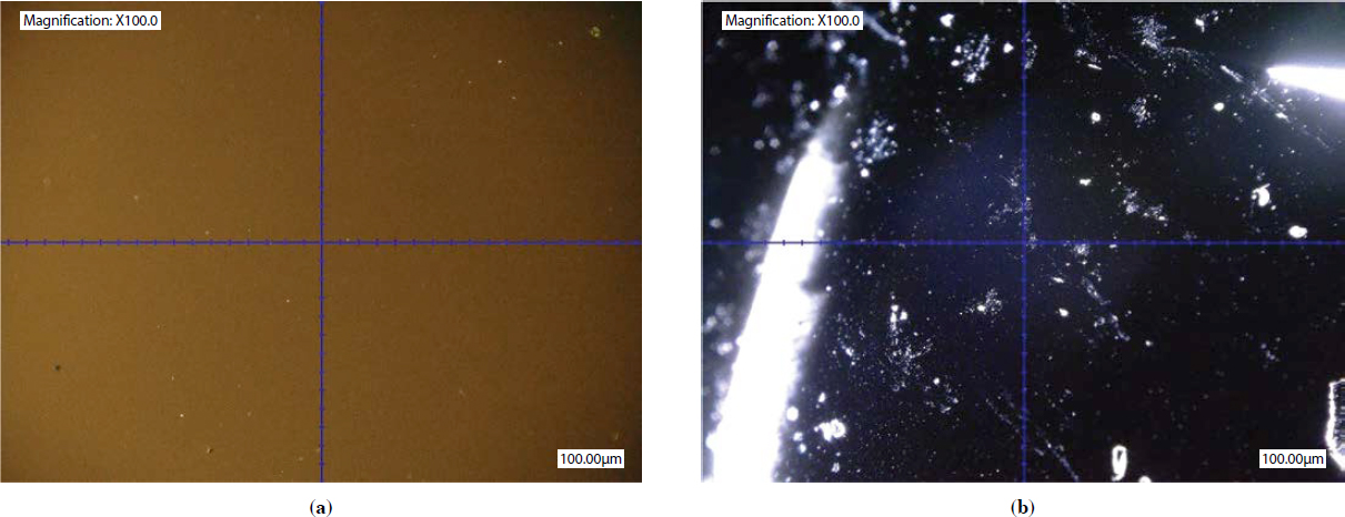

Figure 79 through Figure 81 display microscopy images for the Wisconsin virgin binder, extracted control binder, and extracted RPM binder, respectively. For each of these figures, the image on the left, (a), shows the UV fluorescence microscopy, and the image on the right, (b), shows the darkfield microscopy. The Wisconsin virgin binder showed no fluorescing particles under UV fluorescence microscopy in Figure 79a and no crystallizing materials under darkfield in Figure 79b. The large, bright white portions on the left side and in the center of the image are from artifacts.
The Wisconsin extracted control binder showed some fluorescing particles under UV fluorescence microscopy (Figure 80a). Based on the shape and form of these particles, they are not likely to be associated with specific known polymers or materials observed in the asphalt binder. Thus, they could have originated from the RAP binder in the mixture. However, Figure 80b shows


some scattered, bright white spots under the darkfield, which depict crystallizable fractions present in the sample, probably from the RAP binder. The big white portion in the bottom right of the image in Figure 80b is a reflection of surface artifacts and should be ignored. Furthermore, the halo observed in the middle of the sample is also an artifact, and it occurred due to the intensity of the light source and related reflection from the overall sample surface.
The UV fluorescence microscopy image of the Wisconsin extracted RPM binder in Figure 81a shows some fluorescing particles, similar to Figure 80a but slightly more numerous. The darkfield microscopy image in Figure 81b shows clusters and a network of white spots throughout. The rod-shaped white portion in the center and on the right side of this image is a reflection of surface artifacts and should be ignored.

With detailed comparisons of Figure 79 through Figure 81, it can be inferred that the bright crystalline fractions observed in the Wisconsin extracted RPM binder could be from the RAP binder, any crystalline portion of the aggregates/fines in the new or RAP aggregates, or a portion of the PCR plastics in the mixture. Due to the layered complexity of this matter (i.e., potential presence of fines from aggregate portion, or type and nature of RAP binder as well as fines in the RAP mix), the presence of PCR plastics in the extracted binder cannot be conclusively detected from the microscopy images.
Summary
In summary, the extracted binder results of plant-produced control versus RPM mixtures from the two field projects did not show any distinctive, explainable differences between the mixtures in each project in terms of high and low PG results, viscosities in the typical temperature range for asphalt mixing and compaction, MSCR rutting resistance and elastic properties, black space profiles, LAS fatigue resistance (except for the Ohio project, where the control binder had higher fatigue resistance than the RPM binder), ABCD low-temperature cracking, SARA fractions, and SEC profiles (molecular weight distribution). Furthermore, no conclusive presence of PCR plastics was detected in the RPM binders, based on FTIR results as well as UV fluorescence and darkfield microscopy. The TGA results on post-extraction aggregates indicated the presence of PCR plastics in the case of RPM mixtures.
4.3 Experiment 3: Survey on Recycled Plastics in Asphalt Mixtures and Exploratory QC Testing of PCR Plastics
This section presents responses of asphalt contractors to a survey on using recycled plastics in asphalt mixtures and exploratory QC testing results of PCR plastics using a handheld near-infrared spectrometer in Experiment 3. This information was used as a basis to develop guidelines on sourcing and certification of recycled plastics; QC testing of recycled plastics; and production, construction, and QA testing of dry-process RPM asphalt mixtures, which are presented later in the report.
4.3.1 Survey of Asphalt Contractors on Using Recycled Plastics in Asphalt
According to the survey responses, at least 28 field projects using RPM mixtures have been constructed in the United States since 2018, including 17 projects that used the dry process of adding recycled plastics, while the rest used the wet process or both. The locations of these projects are shown in Figure 82. The survey responses are summarized as follows. (Note: The following list is not an endorsement or recommendation. Other potential suppliers of recycled plastics may be found on the Association of Plastic Recyclers’ website.)
- Suppliers of recycled-plastic materials for these projects included
- – AltiSoro, Houston, TX;
- – Avandgard Innovative, Houston, TX;
- – Domino Plastics Co., Port Jefferson, NY;
- – Ecologic Materials Corp. (now Driven Plastics), Golden, CO;
- – GreenMantra Technologies, Brantford, ON, Canada;
- – Kao Corp., Tokyo, Japan;
- – LyondellBasell, Houston, TX;
- – MacRebur Ltd., Lockerbie, United Kingdom;
- – NVI Advanced Materials Group, St. Louis, MO; and
- – Plastics International, Eden Prairie, MN.

- The most popular forms of RPM plastics were pellets and shreds/flakes. Eleven of the supplied recycled plastics were in pellet form, five were flakes or shredded, and two were in granule/powder form. One project used two suppliers of recycled plastics, and those materials were provided in different forms.
- None of the contractors noted any visible contaminants in the supplied recycled plastics.
- None of the contractors conducted any QC testing of the recycled plastics used in their field trials. A few contractors reported that a cooperating pavement materials research lab had sampled the plastic for further testing, but follow-up correspondence with those labs found that no further testing had been conducted on the supplied plastics.
- Two contractors reported problems with feeding the recycled-plastic material into the plant. One of these contractors used a recycled-plastic material supplied in a fine granule form. The contractor’s existing pneumatic feeder that had been used for cellulose fibers was unable to feed a consistent rate of the plastic granules at the low dosage rate of 5% of virgin binder (0.22% by weight of mixture). It was later discovered that the flexible line that had been feeding the plastic to the mixer had a significant buildup of plastic that hardened in the line.
- All trial projects employed continuous-mix plants. Recycled plastics were added to the plant by a specialty pneumatic feed system (e.g., Hi-Tech Solutions) for 11 of the 17 dry-process projects. The other dry-process projects used some type of hopper and auger system to feed the recycled plastic into the asphalt plant.
- The point of recycled-plastic introduction into the mix production process included RAP entry (11 projects), the same point as asphalt binder (2 projects), “pug mill” (1 project), and with baghouse fines return (1 project).
- Although no projects reported any issues with uniform dispersion of the recycled-plastic material in the mixture, this type of issue may be difficult to detect.
- Eight responses indicated that “no mix or plant adjustments were made,” four indicated that “asphalt content was increased compared to the mix without the recycled plastic,” three indicated that “asphalt content was decreased,” two indicated that “the mix temperature was increased,” and one indicated that “the mix temperature was decreased.”
- Mix temperature at the point of loadout ranged from as low as 143°C (290°F) to 152°C (305°F) at one plant to as high as 166°C (330°F) to 177°C (350°F) at another plant. Most projects reported loadout temperatures of around 166°C (330°F).
- No projects reported any unusual emissions or odors associated with the production of mixes containing recycled plastics.
- Most trial projects indicated that there was “no substantial difference in the way the mix containing recycled plastics handled during paving.” A few projects indicated the mix was more difficult for handwork. One also indicated that there was more buildup on the paver parts and hand tools.
- Regarding compaction, most projects reported no differences compared to the mix without recycled plastics. One reported that the mix containing recycled plastic was a bit tender, but that may have been due to the high mix temperature. Another project reported that the mixture was easier to compact, and yet another reported that “mix temp was critical to achieve density like the old polymer mixes.”
4.3.2 Exploratory QC Testing of PCR Plastics Using Near-Infrared Spectrometer
To determine if the supplied plastic is the expected type and is appropriate for use in asphalt mixture production, a low-cost, handheld near-infrared spectrometer may be useful for QC by contractors. The near-infrared device used in this project was safe and easy to use, and the plastic type was identified in a matter of seconds. Further information on the device can be found elsewhere (BASF, 2024).
Table 19 compares the composition analysis results for FTIR from Experiment 1 versus the near-infrared spectrometer in Experiment 3. The results from the two methods match reasonably well, except for Sample #10. This sample was identified as primarily PET by FTIR but was identified as PE (LDPE) using the near-infrared spectrometer. Despite the promising results obtained, the near-infrared spectrometer has two limitations: (1) It is only capable of detecting the primary composition of the plastic, and thus, it cannot identify secondary components of mixed-stream plastics; and (2) it cannot detect black plastics because the material will absorb all light in the near-infrared spectral region and not provide a sufficient reflected signal for composition detection.
Table 20 summarizes the near-infrared spectrometer results of six PCR plastics for batch-to-batch production consistency evaluation. The results were largely consistent across the 15 production batches for each PCR plastic. The only exception was in the materials from Supplier A,
Table 19. PCR plastic composition analysis results for FTIR versus near-infrared spectrometer.
| PCR Plastic Sample ID | FTIR-Detected Compounds | Near-Infrared Spectrometer | |||||||||
|---|---|---|---|---|---|---|---|---|---|---|---|
| PE | PP | GMS | Slip Agents | PET | Clay | Talc | CaCO3 | Amide I/II | Class | Subclass | |
| #1 | X | O | O | O | PE | LDPE | |||||
| #2 | X | X | X | O | PE | LDPE | |||||
| #3 | X | O | O | O | PE | HDPE | |||||
| #4 | X | X/O | X | O | X/O | PP | NA | ||||
| #5 | X | O | O | X/O | PE | LDPE | |||||
| #6 | X | O | O | O | PE | NA* | |||||
| #7 | X | O | X | X | O | O | O | PE | LDPE | ||
| #8 | X | O | O | PE | LDPE | ||||||
| #9 | X | X/O | O | O | NA† | ||||||
| #10 | X | X | O | PE | LDPE | ||||||
| #11 | X | PET | PET-G‡ | ||||||||
| #12 | X | O | O | NA† | |||||||
Note: Functionality detected via surface scans or transmission scans (designated with X and O, respectively).
*Inconclusive discrimination of HDPE/LDPE.
†Sample is black; its composition cannot be identified by near-infrared spectroscopy.
‡PET-G = polyethylene terephthalate glycol.
Table 20. Batch-to-batch composition analysis using handheld near-infrared spectrometer for six PCR suppliers.
| PCR Plastic Supplier ID | Production Batch ID | Class | Confidence Level (Class) | Subclass | Confidence Level (Subclass) |
|---|---|---|---|---|---|
| A | 1 | PE | High | LDPE | Medium |
| 2 | PE | High | LDPE | High | |
| 3 | PE | High | LDPE | High | |
| 4 | PE | High | LDPE | High | |
| 5 | PE | High | LDPE | High | |
| 6 | PE | High | LDPE | High | |
| 7 | PE | High | HDPE | High | |
| 8 | PE | High | LDPE | High | |
| 9 | PE | High | LDPE | High | |
| 10 | PE | High | LDPE | Medium | |
| 11 | PE | High | LDPE | High | |
| 12 | PE | High | LDPE | Medium | |
| 13 | PE | High | LDPE | Medium | |
| 14 | PE | High | LDPE | High | |
| 15 | PE | High | LDPE | High | |
| B | 1 | PE | High | LDPE | High |
| 2 | PE | High | LDPE | High | |
| 3 | PE | High | LDPE | High | |
| 4 | PE | High | LDPE | High | |
| 5 | PE | High | LDPE | High | |
| 6 | PE | High | LDPE | Medium | |
| 7 | PE | High | LDPE | High | |
| 8 | PE | High | LDPE | High | |
| 9 | PE | High | LDPE | High | |
| 10 | PE | High | LDPE | High | |
| 11 | PE | High | LDPE | High | |
| 12 | PE | High | LDPE | High | |
| 13 | PE | High | LDPE | High | |
| 14 | PE | High | LDPE | High | |
| 15 | PE | High | LDPE | High | |
| C | 1 | PE | High | LDPE | High |
| 2 | PE | High | LDPE | High | |
| 3 | PE | High | LDPE | High | |
| 4 | PE | High | LDPE | High | |
| 5 | PE | High | LDPE | High | |
| 6 | PE | High | LDPE | High | |
| 7 | PE | High | LDPE | High | |
| 8 | PE | High | LDPE | High | |
| 9 | PE | High | LDPE | High | |
| 10 | PE | High | LDPE | High | |
| 11 | PE | High | LDPE | High | |
| 12 | PE | High | LDPE | High | |
| 13 | PE | High | LDPE | High | |
| 14 | PE | High | LDPE | High | |
| 15 | PE | High | LDPE | High | |
| D | 1 | PE | High | LDPE | High |
| 2 | PE | High | LDPE | High | |
| 3 | PE | High | LDPE | Medium | |
| 4 | PE | High | LDPE | High | |
| 5 | PE | High | LDPE | Medium | |
| 6 | PE | High | LDPE | High | |
| 7 | PE | High | LDPE | Medium | |
| 8 | PE | High | LDPE | Medium | |
| 9 | PE | High | LDPE | Medium | |
| 10 | PE | High | LDPE | High | |
| 11 | PE | High | LDPE | High | |
| 12 | PE | High | LDPE | High | |
| 13 | PE | High | LDPE | Medium | |
| 14 | PE | High | LDPE | High | |
| 15 | PE | High | LDPE | High |
| PCR Plastic Supplier ID | Production Batch ID | Class | Confidence Level (Class) | Subclass | Confidence Level (Subclass) |
|---|---|---|---|---|---|
| E | 1 | PE | High | LDPE | High |
| 2 | PE | High | LDPE | Medium | |
| 3 | PE | High | LDPE | High | |
| 4 | PE | High | LDPE | High | |
| 5 | PE | High | LDPE | High | |
| 6 | PE | High | LDPE | Medium | |
| 7 | PE | High | LDPE | High | |
| 8 | PE | High | LDPE | Medium | |
| 9 | PE | High | LDPE | High | |
| 10 | PE | High | LDPE | High | |
| 11 | PE | High | LDPE | High | |
| 12 | PE | High | LDPE | High | |
| 13 | PE | High | LDPE | Medium | |
| 14 | PE | High | LDPE | High | |
| 15 | PE | High | LDPE | High | |
| F | 1 | PE | High | LDPE | High |
| 2 | PE | High | LDPE | High | |
| 3 | PE | High | LDPE | High | |
| 4 | PE | High | LDPE | High | |
| 5 | PE | High | LDPE | High | |
| 6 | PE | High | LDPE | High | |
| 7 | PE | High | LDPE | High | |
| 8 | PE | High | LDPE | High | |
| 9 | PE | High | LDPE | High | |
| 10 | PE | High | LDPE | High | |
| 11 | PE | High | LDPE | High | |
| 12 | PE | High | LDPE | High | |
| 13 | PE | High | LDPE | High | |
| 14 | PE | High | LDPE | High | |
| 15 | PE | High | LDPE | High |
which were identified as LDPE for the compositional “subclass” for all except Batch #7, which was identified as HDPE. The confidence level in Table 20 indicates how well the spectrum of the scanned sample matches a known spectrum in the spectrometer’s database. In summary, the results in Table 19 and Table 20 demonstrate the potential of using the near-infrared spectrometer for QC testing of PCR plastics for production of RPM asphalt mixtures.
4.4 Experiment 4: Selection of Laboratory Method for Adding Recycled Plastics via the Dry Process
This section presents Experiment 4 results comparing the performance properties and fume emissions of laboratory-prepared RPM asphalt mixtures using different methods of adding PCR plastics via the dry process. Based on the results, the most appropriate method of adding PCR plastics was further evaluated in Experiment 5.
4.4.1 Performance Property Comparison of Laboratory-Prepared Control versus RPM Asphalt Mixtures
This section compares the IDEAL-RT, IDEAL-CT, and DCT results of laboratory-prepared control versus RPM asphalt mixtures using four different methods of adding PCR plastics via the dry process. Both mixtures were prepared to simulate the plant-produced mixtures from the two field projects in Experiment 2. The mixtures are labeled based on the field project, PCR plastic–addition method, and mixture type (i.e., laboratory or plant); for example, “WI RPM-LAB Method #1” indicates the Wisconsin RPM mixture prepared using Method 1 in the laboratory,

and “WI Ctrl-LAB” means the Wisconsin control mixture (without PCR plastic) prepared in the laboratory. The Games-Howell group analysis at a significance level of 0.05 was conducted to determine if significant differences existed in the test results for the control versus dry-process RPM mixtures when considering the test variability.
Figure 83 and Figure 84 present the IDEAL-RT results of the laboratory-prepared control and RPM mixtures for the Wisconsin and Ohio projects, respectively. Error bars represent plus and
minus one standard deviation from the average, and capital letters above the bars represent the group analysis results. Mixtures sharing the same letter from the group analysis are not significantly different considering the variability of the replicate results. For the Wisconsin mixtures, two of the mixing methods, WI RPM Lab Method 2 and WI RPM Lab Method 4, yielded RTindex results that were not statistically higher than the corresponding control mixture, which indicates better rutting resistance. For the Ohio mixtures, all four of the mixing methods yielded RTindex results that were statistically higher than the corresponding control mixture.
Figure 85 and Figure 86 present the IDEAL-CT results of the laboratory-prepared control versus RPM mixtures for the Wisconsin and Ohio projects, respectively. For the Wisconsin mixtures, the analysis showed that three of the mixing methods yielded a CTindex statistically equivalent to the corresponding control mixture, which indicates comparable intermediate-temperature cracking resistance. Only Method 2 of laboratory mixing yielded a statistically lower CTindex compared to the control mixture. For the Ohio mixtures, the analysis indicates that four of the mixing methods (Methods 1–4) yielded statistically equivalent CTindex results that were also statistically equal to the corresponding control mixture.
Figure 87 and Figure 88 present the DCT Gf results of the laboratory-prepared control and RPM mixtures for the Wisconsin and Ohio projects, respectively. The group analysis results show that for both Wisconsin and Ohio mixtures, each of the four laboratory mixing methods yielded DCT Gf results that are statistically equivalent to those of the corresponding control mixture.
In summary, the IDEAL-RT, IDEAL-CT, and DCT results indicate that the laboratory-prepared RPM mixtures, regardless of the PCR plastic–addition method used, exhibited better rutting resistance than the control mixture but comparable cracking resistance for both projects. While the IDEAL-RT results demonstrate a mixture-stiffening impact from adding PCR plastics via the dry process, this impact is not evident in the IDEAL-CT and DCT results.


4.4.2 Performance Properties of Plant-Produced versus Laboratory-Prepared RPM Asphalt Mixtures
This section compares the IDEAL-RT, IDEAL-CT, and DCT results of plant-produced versus laboratory-prepared RPM asphalt mixtures for the two field projects in Experiment 2. The laboratory-prepared RPM mixtures were prepared using four different methods of adding PCR plastics discussed previously. The Games-Howell group analysis at a significance level of 0.05 was conducted to statistically compare the results while considering the variability of the test. The group analysis results were used to determine the PCR plastic–addition method that could best mimic the plant production of dry-process RPM mixtures.
Figure 89 and Figure 90 present the IDEAL-RT results of the plant-produced versus laboratory-prepared RPM mixtures for the Wisconsin and Ohio projects, respectively. The plant-produced RPM mixtures had statistically higher RTindex results than all the corresponding laboratory-prepared RPM mixtures. In other words, none of the four PCR plastic–addition methods provided RTindex results that were similar to the RTindex of the corresponding plant-produced mixture.
Figure 91 and Figure 92 present the IDEAL-CT results of the plant-produced versus laboratory-prepared RPM mixtures for the Wisconsin and Ohio projects, respectively. The group analysis results show that for the Wisconsin project, only the mixture prepared with Method 2 has the same statistical group as the plant-produced mixture, whereas for the Ohio project, only the mixture prepared with Method 1 shares the same statistical group as the plant-produced RPM mixture.
The DCT results in Figure 93 and Figure 94 show that, for both the Wisconsin and Ohio projects, the laboratory-prepared and plant-produced RPM mixtures had statistically equivalent Gf results, regardless of the laboratory mixing method. This indicates that either all four mixing methods can simulate the DCT results of plant-produced RPM mixtures, or the DCT results are insensitive to the mixing method.

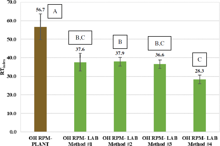


Table 21. Selected PCR plastic–addition method based on group analysis results.
| Project | Performance Test | Selected PCR Plastic–Addition Method Based on Group Analysis Results |
|---|---|---|
| Wisconsin | IDEAL-RT | None |
| IDEAL-CT | Method 2 | |
| DCT | All | |
| Ohio | IDEAL-RT | None |
| IDEAL-CT | Method 1 | |
| DCT | All |
Table 21 summarizes the PCR plastic–addition methods that statistically matched the performance test results of plant-produced RPM mixtures based on the group analysis results. Among the four methods evaluated in the experiment, Method 1 and Method 2 yielded laboratory-prepared RPM mixtures with IDEAL-CT and DCT results that are statistically equivalent to the plant-produced mixture; however, they could not match the IDEAL-RT results.
To better understand the experiment results, IDEAL-CT versus IDEAL-RT diagrams of laboratory-prepared RPM mixtures, using the four mixing methods, versus the plant-produced RPM mixture were plotted for both projects, as shown in Figure 95 and Figure 96. The vertical and horizontal error bars represent plus and minus one standard deviation from the average. The DCT results were not considered in this analysis since there were no statistically significant differences in Gf between the laboratory-prepared and plant-produced RPM mixtures. As shown in Figure 95 and Figure 96, none of the PCR plastic–addition methods could reasonably simulate the production of RPM mixtures at asphalt plants; however, Method 1 is comparatively the best option since it is located closest to the plant-produced RPM mixture in the diagrams.
Similar to the RPM mixtures, large discrepancies were also observed in the IDEAL-CT and IDEAL-RT results for the laboratory-prepared versus plant-produced control mixtures. As shown in Figure 97 and Figure 98, the laboratory-prepared control mixtures were softer than the plant-produced mixtures, as indicated by higher CTindex and lower RTindex results. This trend is consistent with the RPM mixture results in Figure 95 and Figure 96. Therefore, it is hypothesized


that the discrepancy in the IDEAL-CT and IDEAL-RT results between the laboratory-prepared and plant-produced mixtures could be partially due to the difference in asphalt aging from the laboratory short-term aging procedure, per AASHTO R 30, versus the aging that occurred during plant production, followed by approximately 1.5 years of storage in sealed buckets (without temperature control) and mix reheating.
Two additional analyses were explored to determine the most representative method of adding PCR plastics in the laboratory to mimic plant-produced RPM mixtures: (1) comparing the ratio in performance test results of the RPM mixtures over the corresponding control mixture to isolate the effects of adding PCR plastic on the performance test results, and (2) comparing the ratio in performance test results of laboratory-prepared over plant-produced mixtures to eliminate the difference between laboratory mixing and plant production and its impacts on the performance test results. However, both analyses yielded the same conclusion—none of the PCR plastic–addition methods could reasonably match the production of RPM mixtures at asphalt plants.
In summary, the performance test results indicate that none of the four PCR plastic–addition methods simulated the production of RPM mixtures at asphalt plants. Method 1 appeared to be the best option based on the IDEAL-CT versus IDEAL-RT diagram analysis, and it is the most practical and user-friendly method for mix designers in the laboratory. Therefore, it was decided to use Method 1 to prepare dry-process RPM mixtures in the laboratory for performance testing in Experiment 5.
4.4.3 Fume Emission Analysis of Laboratory-Prepared RPM Asphalt Mixtures
This section presents the fume emission results of laboratory-prepared RPM asphalt mixtures using the four different methods of adding PCR plastics via the dry process. The results are organized based on benzene-soluble compounds, PAH compounds, and HAP VOCs, discussed as follows.
Benzene-Soluble Compounds
Table 22 summarizes benzene-soluble compounds obtained on filters for the Ohio and Wisconsin mixtures. All mixtures have no detectable benzene-soluble compounds on filters (i.e., the soluble fraction was under 0.10 mg).
PAH Compounds
Table 23 and Table 24 summarize the PAH compounds obtained on adsorption tubes for the Ohio and Wisconsin mixtures, respectively. No detectable PAH compounds, at a detection limit per EPA TO17 and ISO 16000-6, were found for any of the four mixtures.
Table 22. Gravimetric evaluation of benzene-soluble fraction on filter.
| Mixture ID | PCR Plastic–Addition Method | Total Benzene-Soluble Fraction on Filter (mg) |
|---|---|---|
| OH Control | None | <0.10 |
| OH RPM-1 | Method 1 | <0.10 |
| OH RPM-2 | Method 2 | <0.10 |
| OH RPM-3 | Method 3 | <0.10 |
| OH RPM-4 | Method 4 | <0.10 |
| WI Control | None | <0.10 |
| WI RPM-1 | Method 1 | <0.10 |
| WI RPM-2 | Method 2 | <0.10 |
| WI RPM-3 | Method 3 | <0.10 |
| WI RPM-4 | Method 4 | <0.10 |
Table 23. PAH compounds for Ohio mixtures.
| Compound | Reporting Limit (ng/L) | Sample Concentration (ng/L) | ||||
|---|---|---|---|---|---|---|
| OH Control | OH RPM-1 | OH RPM-2 | OH RPM-3 | OH RPM-4 | ||
| Naphthalene | 5.0 | <5.0 | <5.0 | <5.0 | <5.0 | <5.0 |
| Acenaphthylene | 2.5 | <2.5 | <2.5 | <2.5 | <2.5 | <2.5 |
| Acenaphthene | 2.5 | <2.5 | <2.5 | <2.5 | <2.5 | <2.5 |
| Fluorene | 2.5 | <2.5 | <2.5 | <2.5 | <2.5 | <2.5 |
| Phenanthrene | 2.5 | <2.5 | <2.5 | <2.5 | <2.5 | <2.5 |
| Anthracene | 2.5 | <2.5 | <2.5 | <2.5 | <2.5 | <2.5 |
| Fluoranthene | 2.5 | <2.5 | <2.5 | <2.5 | <2.5 | <2.5 |
| Pyrene | 2.5 | <2.5 | <2.5 | <2.5 | <2.5 | <2.5 |
| Benzo[a]anthracene | 13.0 | <13.0 | <13.0 | <13.0 | <13.0 | <13.0 |
| Chrysene | 13.0 | <13.0 | <13.0 | <13.0 | <13.0 | <13.0 |
| Benzo[b]fluoranthene | 13.0 | <13.0 | <13.0 | <13.0 | <13.0 | <13.0 |
| Benzo[k]fluoranthene | 13.0 | <13.0 | <13.0 | <13.0 | <13.0 | <13.0 |
| Benzo[a]pyrene | 13.0 | <13.0 | <13.0 | <13.0 | <13.0 | <13.0 |
| Indeno[1,2,3-c,d]pyrene | 25.0 | <25.0 | <25.0 | <25.0 | <25.0 | <25.0 |
| Dibenzo[a,h]anthracene | 25.0 | <25.0 | <25.0 | <25.0 | <25.0 | <25.0 |
| Benzo[g,h,i]perylene | 25.0 | <25.0 | <25.0 | <25.0 | <25.0 | <25.0 |
HAP VOCs
Table 25 indicates that four HAP VOCs (i.e., benzene, methylene chloride, toluene, and TCE) were detected from the Ohio fume samples collected during the preparation of the control and RPM mixtures. The monitoring procedure involved pulling 2 L of air through a sorbent packing to collect VOCs, followed by a thermal desorption-capillary GC/mass spectrometry analytical procedure, in accordance with NIOSH Method 2549.
The HAP VOC analysis identified the presence of benzene (a very hazardous compound) at a concentration ranging between 2.5 and 2.8 ng/L in the collected fumes from all samples except the OH RPM-3 mixture, which presented a value below the reporting limit of 2.5 ng/L. All Ohio mixtures presented similar methylene chloride concentrations (between 2.7 and 3.4 ng/L), except the OH RPM-3 mixture, which presented a value below the reporting limit of 2.5 ng/L. In terms of toluene concentration, the mixtures can be separated into three groups: Group 1 includes the OH RPM-3 mixture, with the lowest concentration (46.0 ng/L); Group 2 consists of the OH control and OH RPM-4 mixtures, with intermediate concentrations (between 55.0 and 58.0 ng/L); and Group 3 includes the OH RPM-1 mixture, with the highest concentration (88.0 ng/L).
Table 24. PAH compounds for Wisconsin mixtures.
| Compound | Reporting | Sample Concentration (ng/L) | ||||
|---|---|---|---|---|---|---|
| Limit (ng/L) | WI Control | WI RPM-1 | WI RPM-2 | WI RPM-3 | WI RPM-4 | |
| Naphthalene | 5.0 | <5.0 | <5.0 | <5.0 | <5.0 | <5.0 |
| Acenaphthylene | 2.5 | <2.5 | <2.5 | <2.5 | <2.5 | <2.5 |
| Acenaphthene | 2.5 | <2.5 | <2.5 | <2.5 | <2.5 | <2.5 |
| Fluorene | 2.5 | <2.5 | <2.5 | <2.5 | <2.5 | <2.5 |
| Phenanthrene | 2.5 | <2.5 | <2.5 | <2.5 | <2.5 | <2.5 |
| Anthracene | 2.5 | <2.5 | <2.5 | <2.5 | <2.5 | <2.5 |
| Fluoranthene | 2.5 | <2.5 | <2.5 | <2.5 | <2.5 | <2.5 |
| Pyrene | 2.5 | <2.5 | <2.5 | <2.5 | <2.5 | <2.5 |
| Benzo[a]anthracene | 13.0 | <13.0 | <13.0 | <13.0 | <13.0 | <13.0 |
| Chrysene | 13.0 | <13.0 | <13.0 | <13.0 | <13.0 | <13.0 |
| Benzo[b]fluoranthene | 13.0 | <13.0 | <13.0 | <13.0 | <13.0 | <13.0 |
| Benzo[k]fluoranthene | 13.0 | <13.0 | <13.0 | <13.0 | <13.0 | <13.0 |
| Benzo[a]pyrene | 13.0 | <13.0 | <13.0 | <13.0 | <13.0 | <13.0 |
| Indeno[1,2,3-c,d]pyrene | 25.0 | <25.0 | <25.0 | <25.0 | <25.0 | <25.0 |
| Dibenzo[a,h]anthracene | 25.0 | <25.0 | <25.0 | <25.0 | <25.0 | <25.0 |
| Benzo[g,h,i]perylene | 25.0 | <25.0 | <25.0 | <25.0 | <25.0 | <25.0 |
Table 25. HAP VOCs for Ohio mixtures.
| Compound | Reporting Limit (ng/L) | Sample Concentration (ng/L) | ||||
|---|---|---|---|---|---|---|
| OH Control | OH RPM-1 | OH RPM-2 | OH RPM-3 | OH RPM-4 | ||
| Benzene | 2.5 | 2.6 | 2.8 | 2.5 | <2.5 | 2.7 |
| Methylene chloride | 2.5 | 3.4 | 3.2 | 2.7 | <2.5 | 3.2 |
| Toluene | 2.5 | 55.0 | 88.0 | 68.0 | 46.0 | 58.0 |
| TCE | 2.5 | 200.0 | 270.0 | 230.0 | 160.0 | 210.0 |
For TCE, it was observed that the OH RPM-3 mixture showed the lowest value (160.0 ng/L), followed by the OH control, OH RPM-4, and OH RPM-2 mixtures (ranging between 200.0 and 230.0 ng/L), while the OH RPM-1 mixture presented the highest value (270.0 ng/L). Thus, the OH RPM-3 method produced the lowest concentrations of the four HAP VOCs. As the OH control mixture presented the same HAP VOCs as the PCR mixtures, it was concluded that the PCR plastics were not the source of the detected HAP VOCs.
Table 26 presents the occupational exposure limits (OELs) required by the Occupational Safety and Health Administration (OSHA) for the four HAP VOCs (i.e., benzene, methylene chloride, toluene, and TCE) detected among the Ohio mixtures. An OEL is representative of the highest concentration of a chemical substance that a healthy worker can be exposed to. Two OSHA OELs are being considered in this analysis of the airborne concentration of the found VOCs: 8-hour time-weighted average (TWA) exposure limit and 15-minute short-term exposure limit (STEL). The concentration of each HAP VOC detected among the Ohio mixtures was significantly below the OSHA TWA and STEL values.
Table 27 indicates that three HAP VOCs (i.e., methylene chloride, toluene, and TCE) were detected from the Wisconsin fume samples collected during the preparation of the control and RPM mixtures using different dry-process PCR plastic–addition methods.
Table 26. OSHA TWA and STEL values—HAP VOCs for Ohio mixtures.
| Compound | OSHA Exposure Limit (ppm) | Sample Concentration (ppm) | |||||
|---|---|---|---|---|---|---|---|
| TWA (8-hour OEL) | STEL (15-min. OEL) | OH Control | OH RPM-1 | OH RPM-2 | OH RPM-3 | OH RPM-4 | |
| Benzene | 1.0* | 5.0* | 0.0008 | 0.0009 | 0.0008 | <0.0008 | 0.0008 |
| Methylene chloride | 25.0† | 125.0† | 0.001 | 0.0009 | 0.0008 | <0.0007 | 0.0009 |
| Toluene | 100.0‡ | 150.0‡ | 0.014 | 0.023 | 0.018 | 0.012 | 0.015 |
| TCE | 100.0§ | 200.0§ | 0.036 | 0.05 | 0.042 | 0.029 | 0.038 |
*Per OSHA 1910.1028.
†Per OSHA 1910.1052.
‡Per OSHA (n.d.).
§Per OSHA (2021).
Table 27. HAP VOCs for Wisconsin mixtures.
| Compound | Reporting Limit (ng/L) | Sample Concentration (ng/L) | ||||
|---|---|---|---|---|---|---|
| WI Control | WI RPM-1 | WI RPM-2 | WI RPM-3 | WI RPM-4 | ||
| Benzene | 2.5 | <2.5 | <2.5 | <2.5 | <2.5 | <2.5 |
| Methylene chloride | 2.5 | 4.4 | 5.4 | 3.2 | 5.0 | 3.8 |
| Toluene | 2.5 | 10.0 | 12.0 | 78.0 | 9.8 | 8.0 |
| TCE | 2.5 | 920.0 | 1,100.0 | 370.0 | 890.0 | 750.0 |
Table 28. OSHA TWA and STEL values—HAP VOCs for Wisconsin mixtures.
| Compound | OSHA Exposure Limit (ppm) | Sample Concentration (ppm) | |||||
|---|---|---|---|---|---|---|---|
| TWA (8-hour OEL) | STEL (15-min. OEL) | WI Control | WI RPM-1 | WI RPM-2 | WI RPM-3 | WI RPM-4 | |
| Benzene | 1.0* | 5.0* | <0.0008 | <0.0008 | <0.0008 | <0.0008 | <0.0008 |
| Methylene chloride | 25.0† | 125.0† | 0.0012 | 0.0015 | 0.0009 | 0.0014 | 0.0011 |
| Toluene | 100.0‡ | 150.0‡ | 0.0027 | 0.0032 | 0.02 | 0.0026 | 0.0021 |
| TCE | 100.0§ | 200.0§ | 0.17 | 0.19 | 0.067 | 0.16 | 0.14 |
*Per OSHA 1910.1028.
†Per OSHA 1910.1052.
‡Per OSHA (n.d.).
§Per OSHA (2021).
No detectable benzene, at a detection limit of 2.5 ng/L, was found for the Wisconsin mixtures. All mixtures showed similar methylene chloride values (between 3.2 and 5.4 ng/L). Similar values for toluene concentration were also found among the Wisconsin mixtures (between 8.0 and 12.0 ng/L) except for the WI RPM-2 mixture, which showed the highest concentration at 78.0 ng/L. In terms of TCE concentration, the mixtures can be separated into three groups: Group 1 includes the WI RPM-2 mixture, with the lowest concentration (370.0 ng/L); Group 2 consists of the WI RPM-3 and WI RPM-4 mixtures, with intermediate concentrations (between 750.0 and 890.0 ng/L); and Group 3 includes the WI control and WI RPM-1 mixtures, with the highest concentrations (between 920.0 and 1,100.0 ng/L). Among all evaluated mixing procedures, the WI RPM-2 procedure produced the lowest concentration of methylene chloride and TCE, while the WI RPM-4 procedure produced the lowest concentration of toluene. Due to the WI control mixture having the same HAP VOCs as the PCR mixtures, it was concluded that the PCR plastics were not the source of the found HAP VOCs.
Table 28 presents the TWA and STEL required by OSHA for the HAP VOCs found among the Wisconsin mixtures. The detected concentration of each HAP VOC was significantly below the OSHA TWA and STEL values.
Table 29 presents the VOCs found in the laboratory screening of the PCR plastics through direct headspace-GC analysis in Experiment 1 (see detailed results earlier in this chapter). None of the HAP VOCs (i.e., benzene, methylene chloride, and TCE) detected during the preparation of control and dry-process RPM mixtures were found in the laboratory screening of the PCR plastics—this points to the virgin asphalt binder or the RAP as the potential origin of the HAP VOCs presented in the fume samples.
The VOC analysis was then conducted on the virgin asphalt binder, and the results are presented in Table 30. As is typical for straight-run asphalts, benzene and toluene HAP VOCs were
Table 29. VOCs detected in the PCR plastics used in Ohio and Wisconsin field projects.
| Field Project | PCR Plastic ID | Compound | Sample Concentration (µg/g) |
|---|---|---|---|
| Ohio | #5 | Benzenesulfonamide, N-butyl- | 0.29 |
| Boric acid, trimethyl ester | 1.19 | ||
| Ethanedioic acid, dibutyl ester | 0.46 | ||
| Hexane, 2,2,4-trimethyl- | 1.44 | ||
| Wisconsin | #2 | Benzenesulfonamide, N-butyl- | 0.27 |
| Heptane, 2,2-dimethyl- | 0.73 | ||
| Limonene | 0.85 |
Table 30. VOCs detected in the virgin asphalt binders used in the Ohio and Wisconsin field projects.
| Field Project | Compound | Sample Concentration (μg/g) |
|---|---|---|
| Ohio | 3,4-Hexanedione, 2,2,5-trimethyl- | 0.68 |
| Acetyl valeryl | 0.64 | |
| Benzene | 0.06 | |
| Carbonic acid, ethyl 2-propenyl ester | 0.68 | |
| Methacrolein | 0.34 | |
| Octacosane | 0.61 | |
| Oxalic acid, allyl isobutyl ester | 0.57 | |
| Toluene | 0.25 | |
| Wisconsin | Acetic acid | 1.29 |
| Acetone | 3.05 | |
| Acetyl valeryl | 0.63 | |
| Benzene | 0.07 | |
| Benzene, 1-ethyl-2-methyl- | 0.57 | |
| Benzene, (1-methylpropyl)- | 1.63 | |
| Benzene, 1,4-diethyl- | 2.65 | |
| Benzene, 1-methyl-2-(1-methylethyl)- | 2.07 | |
| Carbonic acid, ethyl 2-propenyl ester | 0.69 | |
| Cyclotrisiloxane, hexamethyl- | 0.25 | |
| Di-ethyleneglycol, di-formyl- | 0.79 | |
| Ethene, ethoxy- | 0.75 | |
| Hexanal | 0.91 | |
| Hexane, 2,3-dimethyl- | 0.63 | |
| Octacosane | 1.02 | |
| Toluene | 0.37 | |
| 1-Hexanone, 5-methyl-1-phenyl- | 0.50 | |
| 1,2,3,5-Tetramethylbenzene | 1.01 | |
| 1,2,4,5-Tetramethylbenzene | 1.76 |
detected, but methylene chloride and TCE were not detected. Although it is conceivable that the methylene chloride and TCE fumes from the PCR plastic mixtures could have originated while blending a chlorinated polymer into the virgin asphalt at elevated temperatures, it seems more likely that the RAP could be the source of the two chlorinated compounds identified in the fumes released during mixture production in the laboratory.
Summary
The fume emission results indicate that adding PCR plastics via the dry process (regardless of which method of addition was used) did not create or release meaningful amounts of hazardous fumes, and PAHs were not present in those fumes. Only a limited number of HAP VOCs (including benzene, methylene chloride, and TCE) were produced from the mixing process, and all the HAP VOCs detected were also present in the control mixtures. Therefore, the PCR plastics likely did not introduce new compounds to the fumes, but they may have changed the observed concentrations of the compounds in the fumes. Nonetheless, the concentrations of the detected HAP VOCs were significantly below the OSHA TWA and STEL values.
4.5 Experiment 5: Laboratory Characterization of Laboratory-Prepared RPM versus Control Asphalt Mixtures and Extracted Binders
The following sections present the results of Experiment 5, which compared the performance properties and surface characteristics of laboratory-prepared RPM mixtures with different PCR plastics versus the control mixtures using two asphalt mix designs, as well as the analysis results for correlating the PCR plastic properties to RPM mixture properties.
4.5.1 Southern Mix Design Results
This section presents the mixture test results of the control mixture and five dry-process RPM mixtures for the southern mix design. The control mixture is denoted as S-Ctrl, and the five RPM mixtures are denoted as S-RPM1, S-RPM2, S-RPM5, S-RPM7, and S-RPM9, respectively, according to the Sample IDs of the selected PCR plastics in Table 13. The Games-Howell post-hoc test (i.e., group analysis) at a significance level of 0.05 was conducted to statistically compare the results of the control versus RPM mixtures for the DWT, IDEAL-RT, IDEAL-CT, and DCT test. Any two mixtures sharing the same letter from the group analysis are not significantly different considering the variability of the test results.
Mixture Workability
Figure 99 presents the DWT results at three different temperatures: (a) 107°C (225°F), (b) 121°C (250°F), and (c) 135°C (275°F). Error bars represent plus and minus one standard deviation from the average, and capital letters above the bars represent the group analysis results. The DWT values generally increased with testing temperature across mixtures, indicating improved mixture workability at higher temperatures. In most cases, the five RPM mixtures exhibited lower average DWT values compared to the control mixture at the same testing temperature. This indicates that the RPM mixtures required higher compaction efforts due to the increased stiffness from the addition of PCR plastics, thus rendering them less workable and compactible than the control mixture. However, according to the group analysis, the differences in DWT results between the control and RPM mixtures were not statistically significant in all cases except one (i.e., S-RPM9 at 107°C) when considering the variability of the test results.
Mixture Stiffness and Aging Resistance
Figure 100 presents the |E*| master curves at the (a) short-term aging and (b) critical aging conditions. The control and RPM mixtures had comparable |E*| values at low temperatures and high frequencies (right-hand side of the master curve) at both aging conditions, but their |E*| values differed at high temperatures and low frequencies (left-hand side of the master curve), especially at the short-term aging condition. The |E*| results show that adding PCR plastics via the dry process had a stiffening impact on laboratory-prepared mixtures, which is consistent with the findings of Experiment 2 for plant-produced mixtures.
Figure 101 presents the G-Rm results by considering the |E*| and phase angle at 20°C and 5 Hz, where a lower G-Rm value is desired for asphalt mixtures with reduced brittleness and potentially less susceptibility to block cracking. At both aging conditions, the RPM mixtures consistently exhibited G-Rm values that were comparable to or higher than the control mixture. Among the five RPM mixtures, S-RPM5 and S-RPM7 had lower G-Rm values than the others, possibly due to differences in the properties of the PCR plastics. Figure 102 presents the G-Rm ratio results at the critical aging over short-term aging conditions. The control mixture had the highest G-Rm ratio; thus, it was expected to be more susceptible to aging than the RPM mixtures. The G-Rm results indicate that adding PCR plastics via the dry process reduced the block cracking resistance but improved the aging resistance of asphalt mixtures, with varying impacts among different PCR plastics.
Mixture Rutting Resistance
Figure 103 presents the HWTT rut depth curves at 50°C. A lower rut depth signifies better rutting resistance. All five RPM mixtures had slightly lower rut depth than the control mixture, indicating better rutting resistance due to a stiffening impact from adding PCR plastics. However, this improvement may not be practically significant, considering that all the mixtures had minimal rutting (i.e., less than 4 mm) with no signs of stripping.


Figure 104 presents the IDEAL-RT results, with the error bars representing plus and minus one standard deviation from the average RTindex and the letters above the bars representing the group analysis results. The test was conducted at 64°C, a common high-temperature performance grade in the southern United States per LTPPBind. Mixtures with higher RTindex are expected to have better rutting resistance. Three out of five RPM mixtures exhibited higher average RTindex values than the control mixture, while the other two exhibited slightly lower average RTindex values. However, these differences were not statistically significant considering the variability of the test results, according to the group analysis. Overall, the HWTT and IDEAL-RT results show that the rutting resistance for dry-process RPM mixtures was slightly better than or equivalent to the control mixture for the southern mix design.
Mixture Moisture Susceptibility
Figure 105 presents the TSR results. Two RPM mixtures (S-RPM1 and S-RPM9) had practically higher TSR values than the control mixture per a d2s limit of 9.3% (Azari, 2010), while


the others were considered equivalent to the control mixture. Thus, adding dry-process PCR plastics at 0.5% dosage did not have a detrimental impact on the moisture resistance of the southern mix design.
Mixture Cracking Resistance
Figure 106 presents the IDEAL-CT results at 25°C, where a higher CTindex is desired for better intermediate-temperature cracking resistance. All five RPM mixtures had lower average CTindex values than the control mixture, indicating reduced cracking resistance due to adding PCR plastics via the dry process. Nevertheless, the group analysis shows that the differences were not statistically significant considering the variability of the test results. Overall, the IDEAL-CT results show that adding dry-process PCR plastics at 0.5% dosage did not significantly reduce the intermediate-temperature cracking resistance of the southern mix design.
Figure 107 presents the C-versus-S curves from the CF test. All the RPM mixtures except S-RPM2 and S-RPM7 had lower fatigue damage tolerance (as indicated by shorter C-versus-S

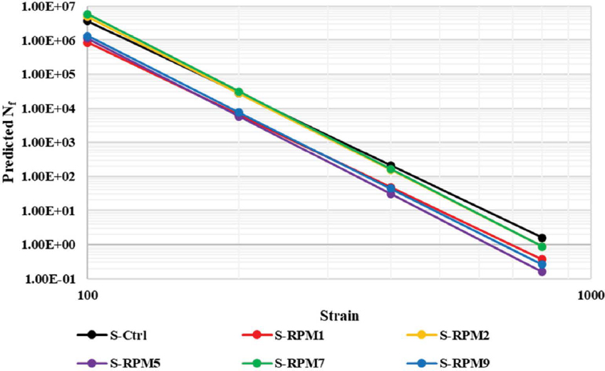
curves) than the control mixture. Similar trends were observed for the predicted Nf-versus-strain results in Figure 108, where the control mixture showed significantly better fatigue resistance (as indicated by higher predicted Nf values over a wide range of strain levels) than all the dry-process RPM mixtures except S-RPM2 and S-RPM7. Finally, Figure 109 presents the CF results using Sapp. All RPM mixtures had lower Sapp values than the control mixture, indicating a detrimental impact of adding dry PCR plastics on the fatigue resistance of the southern mix design. However, this impact varied among the different PCR plastics, as indicated by the significantly lower Sapp values for S-RPM1, S-RPM5, and S-RPM9 (ranging from 8.9 to 10.9) compared to S-RPM2 and S-RPM7 (ranging from 13.5 to 14.1).
To compare the IDEAL-CT and CF test results, a graph of the average CTindex versus Sapp values is presented in Figure 110. Despite their distinct mechanisms, both tests showed a consistent


trend: Adding PCR plastics via the dry process adversely impacted the cracking resistance of the southern mix design. However, the impact varied among different PCR plastics, and in some cases, the impact was shadowed by the variability of the test.
Figure 111 presents the DCT Gf results at −12°C, where a higher Gf is desired for better low-temperature cracking resistance. The test was conducted at −12°C because it is 10°C higher than the most common low-temperature performance grade of the southern United States per LTPPBind (i.e., −22°C). All five RPM mixtures had higher average Gf than the control mixture, indicating improved low-temperature cracking resistance. However, the group analysis shows that the differences were not statistically significant considering the variability of the test results. The DCT results were also analyzed using the FST parameter, which showed trends that resemble those of the Gf results. Overall, the DCT results indicate that adding dry-process PCR plastics


at 0.5% dosage did not significantly impact the low-temperature cracking resistance of the southern mix design.
Mixture Surface Texture and Friction
Figure 112 and Figure 113 present the CTM and DFT results of the southern mix design, respectively. As seen in Figure 112, the control, S-RPM2, and S-RPM9 mixtures showed an increase in MPD after the first 50,000 polishing cycles and 333 hours of NAWS aging, which generally remained consistent over the remaining rounds of polishing and weathering. For the other three

RPM mixtures (i.e., S-RPM1, S-RPM5, and S-RPM7), the MPD continued to increase during the 100,000 polishing cycles and 666 hours of NAWS aging, then kept consistent with additional polishing and NAWS weathering. Visual inspection of the slabs suggested that the increase in MPD was caused by the loss of fine particles during surface polishing and weathering. All RPM mixtures except S-RPM5 had considerably higher final MPD (after 150,000 polishing cycles and 1,000 hours of NAWS aging) than the control mixture.
The friction results in Figure 113 show that the DFT40 first increased after 50,000 polishing cycles and 333 hours of NAWS aging and then decreased for the control, S-RPM1, and S-RPM5 mixtures. Conversely, the S-RPM2, S-RPM7, and S-RPM9 mixtures generally had consistent DFT40 values throughout the polishing and NAWS weathering process. All five RPM mixtures exhibited slightly higher DFT40 values than the control mixture after 150,000 polishing cycles and 1,000 hours of NAWS weathering, but the differences were not considered practically significant. Overall, the DFT results indicate that adding PCR plastics via the dry process did not affect the surface friction of the southern mix design.
Extracted Binder FTIR
Asphalt binders were extracted and recovered from the control and dry-process RPM mixtures prepared with the southern mix design, following the same procedure used in Experiment 2 (see Chapter 3). The extracted binders were then fingerprinted with FTIR to detect the presence of plastics. Figure 114 shows the FTIR results with two solvents: CS2 and TCE. TCE runs were performed specifically to detect the methyl and methylene groups from the polymers in plastics. The peak at around 1,377 cm−1 (Figure 114a) represents the methyl (CH3, C-H bend) umbrella that should be enriched in samples with plastics. The peak at around 1,457 cm−1 (Figure 114b) corresponds to the methylene (CH2, C-H bend) umbrella that should be highly enriched in polyethylene and polypropylene polymers. For both solvents, the extracted control and RPM binders had almost overlapping absorptance spectra, indicating no appreciable presence of PCR plastics in the RPM binders. Given this finding, no further rheological or chemical testing was conducted on the extracted control and RPM binders.
Summary
The mixture performance test results indicate that, overall, the dry-process RPM mixtures prepared with the southern mix design exhibited workability, intermediate-temperature cracking resistance, and low-temperature cracking resistance comparable to the control mixture, as indicated by the DWT, IDEAL-CT, and DCT results, respectively. The RPM mixtures demonstrated slightly improved or similar rutting and moisture resistance (based on the HWTT, IDEAL-RT, and TSR results) but reduced or similar fatigue damage resistance (based on the CF test results) compared to the control mixture. The |E*| and G-Rm results showed that the RPM mixtures had higher stiffness and brittleness than the control mixture, which could lead to increased susceptibility to block cracking. Nevertheless, the RPM mixtures had consistently lower G-Rm ratios at the critical aging over the short-term aging conditions; thus, they could have better aging resistance than the control mixture. Finally, the RPM mixtures had higher MPD and similar DFT40 after surface polishing and NAWS weathering compared to the control mix, indicating that adding PCR plastics via the dry process had no detrimental impacts on the surface texture and friction of asphalt mixtures. FTIR testing of extracted binders from the RPM mixtures showed no appreciable presence of PCR plastics, which agrees with the findings of Experiment 2.
4.5.2 Northern Mix Design Results
This section presents the mixture test results of the control and five dry-process RPM mixtures for the northern mix design. The control mixture is denoted as N-Ctrl, and the five RPM

mixtures are denoted as N-RPM1, N-RPM2, N-RPM5, N-RPM7, and N-RPM9, respectively, according to the Sample ID of the selected PCR plastics in Table 13. The Games-Howell post-hoc test (i.e., group analysis) at a significance level of 0.05 was conducted to statistically compare the results of the control versus RPM mixtures for the DWT, IDEAL-RT, IDEAL-CT, and DCT test. Any two mixtures sharing the same letter from the group analysis are not significantly different considering the variability of the test results.
Mixture Workability
Figure 115 presents the DWT results at three different temperatures: 107°C (225°F), 121°C (250°F), and 135°C (275°F). Except for N-RPM2 and N-RPM9, the RPM mixtures had similar DWT values at all three test temperatures. N-RPM2 and N-RPM9 had statistically lower DWT values at 121°C (250°F), which indicates that certain recycled plastics can negatively impact the workability of asphalt mixtures. However, the grouping analysis results show that the difference in the DWT results between the control and the RPM mixtures was not statistically significant in all cases except two (i.e., N-RPM2 and N-RPM9 at 121°C).
Mixture Stiffness and Aging Resistance
Figure 116 presents the |E*| master curves at two aging conditions. All mixtures had comparable |E*| values at the short-term aging condition. After critical aging, however, two out of five RPM mixtures had notably higher |E*| values at high temperatures and low frequencies (left-hand side of the master curve) than the control mixture, indicating a stiffening impact from adding PCR plastics via the dry process.
Figure 117 presents the G-Rm results at 20°C and 5 Hz. In most cases, the RPM mixtures had higher G-Rm than the control mixture, indicating increased brittleness and potentially increased susceptibility to block cracking. However, the G-Rm ratio results in Figure 118 do not show a consistent trend in the aging resistance of the five RPM versus control mixtures, which differs from the southern mix design results in Figure 102.
Mixture Rutting Resistance
Figure 119 presents the HWTT rut depth curves at 46°C. The RPM mixtures showed significantly better rutting and stripping resistance compared to the control mixture, as indicated by lower rut depth and delayed onset of the stripping phase. These improvements could be attributed to the stiffening impact of adding PCR plastics via the dry process.
Figure 120 presents the IDEAL-RT results at 58°C, where a higher RTindex is desired for asphalt mixtures with better rutting resistance. The test temperature was selected based on the high-temperature performance grade of the northern United States, according to LTPPBind. All RPM mixtures exhibited higher average RTindex values than the control mixture, indicating improved rutting resistance. However, the grouping analysis shows that in some cases, the differences between the control and RPM mixtures were not statistically significant if considering the variability of the test results. Overall, the HWTT and IDEAL-RT results show that adding PCR plastics via the dry process improved the rutting resistance of the northern mix design, but the improvement varied among different PCR plastics.
Mixture Moisture Susceptibility
Figure 121 presents the TSR results. All the RPM mixtures had lower TSR values than the control mixture, but the difference between the control and N-RPM2 mixtures was not practically significant according to the TSR d2s limit of 9.3%. Overall, the TSR results show that adding PCR plastics via the dry process had a detrimental impact on the moisture resistance of the northern mix design.


Mixture Cracking Resistance
Figure 122 presents the IDEAL-CT results at 25°C, where a higher CTindex is desired for better intermediate-temperature cracking resistance. There was no consistent trend when comparing the control versus RPM mixtures. Three out of five RPM mixtures exhibited higher average CTindex values than the control mixture, while the other two had slightly lower average CTindex values. However, these differences were not statistically significant if considering the variability of the test results. Therefore, the IDEAL-CT results indicate that adding dry-process PCR plastics at 0.5% dosage did not show a significant impact on the intermediate-temperature cracking resistance of the northern mix design.


Figure 123 presents the CF results using Sapp. In all cases except one, the RPM mixtures had lower Sapp values than the control mixture, indicating reduced fatigue resistance. Nevertheless, the differences between the control and N-RPM1, N-RPM2, and N-RPM5 mixtures might not be practically significant. Figure 124 depicts the plot of CTindex versus Sapp results for the northern mix design. The two tests did not reveal a consistent trend when comparing the cracking resistance of the control versus RPM mixtures containing different PCR plastics. Finally, Figure 125 and Figure 126 present the C-versus-S curves and predicted Nf-versus-strain curves, respectively, from the CF test, where the control mixture showed a level of fatigue resistance that was better than or comparable to the RPM mixtures.


Figure 127 presents the DCT Gf results at −18°C, where a higher Gf is desired for better low-temperature cracking resistance. The test temperature of −18°C was selected because it is 10°C higher than the most common low-temperature performance grade of the northern United States per LTPPBind (i.e., −28°C). According to the group analysis, all RPM mixtures had Gf results that were similar to those of the control mixture, which indicates that adding dry-process PCR plastics at 0.5% dosage did not significantly impact the low-temperature cracking resistance of the northern mix design. The DCT results were also analyzed using the FST parameter, and the results yielded the same conclusions as the Gf results.

Mixture Surface Texture and Friction
Figure 128 and Figure 129 present the CTM and DFT results, respectively, where the control and RPM mixtures showed similar trends with surface polishing and NAWS weathering. After 150,000 cycles of polishing and 1,000 hours of NAWS weathering, all five RPM mixtures showed MPD and DFT40 results comparable to those of the control mixture, which indicates that adding PCR plastics via the dry process did not have a significant impact on the surface texture and friction of the northern mix design.
Extracted Binder FTIR
Asphalt binders were extracted and recovered from the control and dry-process RPM mixtures prepared with the northern mix design, following the same procedure used in Experiment 2 (see Chapter 3). The extracted binders were then fingerprinted with FTIR to detect the presence of plastics. Figure 130 shows the FTIR results on the extracted binders with CS2 as solvent. The peak at around 1,377 cm−1 exhibits the methyl (CH3, C-H bend) umbrella that should be enriched in the asphalt binders containing PCR plastics. Based on the FTIR data, it can be inferred that there was no appreciable presence of PCR plastics in the extracted RPM binders. Given this finding, no further rheological or chemical testing was conducted on the extracted control and RPM binders (including FTIR with TCE as solvent).
Summary
The mixture performance test results indicate that, overall, the dry-process RPM mixtures prepared with the northern mix design exhibited workability, intermediate-temperature cracking resistance, and low-temperature cracking resistance comparable to the control mixture, as indicated by the DWT, IDEAL-CT, and DCT results, respectively. Most RPM mixtures showed improved rutting resistance in the HWTT and IDEAL-RT but reduced fatigue damage resistance and moisture resistance in the CF and TSR tests, respectively, but the impacts varied depending on the PCR plastics used. The |E*| and G-Rm results showed that the RPM mixtures exhibited


higher stiffness and brittleness than the control mixture, which could lead to increased susceptibility to block cracking. Finally, the RPM mixtures and control mixture both had similar MPD and DFT40 results after surface polishing and NAWS weathering. FTIR testing of extracted binders from the RPM mixtures showed no appreciable presence of PCR plastics, which agrees with the southern mix design results and findings of Experiment 2.
4.5.3 Correlation of PCR Plastic Properties versus RPM Mixture Results
This section presents analyses of possible correlations between the PCR plastic properties and the mixture performance results of both southern and northern mix designs. Pearson’s correlation coefficient (rp) was used to evaluate the strength and direction of the correlation, where (1) rp varies between −1.0 and +1.0, and (2) a positive rp indicates positive correlation while a negative rp indicates negative correlation (Chen et al., 2022). A greater absolute value of rp demonstrates a stronger correlation. In general, an |rp| of 0.6 to 0.8 implies a strong linear correlation, and an |rp| of 0.8 to 1.0 implies a very strong linear correlation (Evans, 1996). Table 31 summarizes the PCR plastic properties and the mixture performance test parameters used in the correlation analysis.
Table 32 summarizes the correlation rp results for both mix designs. The correlations between the PCR plastic properties and mixture performance test results were considered strong when the following two conditions were met: (1) the |rp| value was greater than 0.6 for both mix designs, and (2) the rp value showed the same correlation direction for both mix designs (i.e., both positive or both negative). As highlighted in Table 32, among the various PCR plastic properties included in the correlation analysis, MFI had strong correlations with the mixture test results for DWT at 121°C (250°F), G-Rm, RTindex, and HWTT rut depth, and initial melting temperature correlated well with DWT results.
Figure 131 and Figure 132 present the critically aged G-Rm and IDEAL-RT correlation results, respectively, as illustration examples, where the blue dashed line in each figure represents the result of the control mixture without PCR plastics. All the RPM mixtures, regardless of the mix design and PCR plastics used, had higher or similar G-Rm values and RTindex results compared to the control mixture, indicating increased mixture brittleness, susceptibility to block cracking, and rutting resistance. According to the correlation results, these impacts were more pronounced for mixtures containing PCR plastics with higher MFI. The research team’s hypothesis for this phenomenon is that PCR plastics with higher MFI have relatively lower viscosities (i.e., flow resistance); thus, they are more likely to melt when added via the dry process, which will stiffen the asphalt binder and increase the brittleness, block cracking susceptibility, and rutting resistance of the resultant mixture.
Table 31. List of PCR plastic properties and mixture performance test parameters used for correlation analysis.
| PCR Plastic Properties | Mixture Performance Test Parameters |
|---|---|
|
|
Table 32. Pearson correlation analysis coefficients.
| PCR Plastic Property | Mix Design | DWT (ºF) | G-Rm (MPa) | IDEAL-RT RTindex | Rut Depth (mm) | TSR (%) | IDEAL-CT CTindex | Gf (J/m2) | Sapp | |||
|---|---|---|---|---|---|---|---|---|---|---|---|---|
| 225 | 250 | 275 | STOA* | CA | ||||||||
| MFI | Southern | -0.741 | -0.857 | -0.150 | 0.706 | 0.816 | 0.990 | -0.923 | 0.681 | -0.575 | -0.787 | -0.232 |
| Northern | -0.513 | -0.869 | -0.891 | 0.924 | 0.986 | 0.784 | -0.609 | -0.293 | -0.772 | 0.407 | 0.723 | |
| GPC weight-average molecular weight, Mw x 103 | Southern | 0.374 | 0.383 | 0.629 | -0.544 | -0.733 | -0.294 | 0.217 | -0.730 | 0.142 | 0.801 | 0.654 |
| Northern | 0.326 | -0.049 | 0.082 | -0.266 | -0.346 | -0.787 | 0.521 | 0.345 | 0.844 | -0.936 | -0.115 | |
| Specific gravity | Southern | -0.278 | -0.443 | 0.246 | -0.021 | -0.049 | 0.458 | -0.579 | -0.022 | -0.395 | 0.083 | 0.251 |
| Northern | -0.136 | -0.730 | -0.516 | 0.479 | 0.395 | -0.173 | 0.182 | 0.044 | 0.187 | -0.435 | 0.641 | |
| Pellet count (per gram) | Southern | -0.035 | -0.532 | -0.367 | -0.245 | 0.096 | 0.250 | -0.357 | 0.728 | 0.005 | -0.495 | -0.793 |
| Northern | 0.190 | -0.198 | 0.036 | 0.161 | 0.254 | 0.066 | 0.418 | -0.729 | -0.189 | 0.481 | 0.816 | |
| DSC initial crystallization temperature, Tc1 (ºC) | Southern | -0.446 | -0.545 | 0.335 | 0.317 | 0.288 | 0.773 | -0.736 | 0.146 | -0.435 | -0.212 | 0.247 |
| Northern | -0.254 | -0.875 | -0.829 | 0.712 | 0.735 | 0.232 | -0.263 | -0.057 | -0.173 | -0.266 | 0.595 | |
| DSC initial melting temperature, Tm1 (ºC) | Southern | -0.434 | -0.677 | 0.166 | 0.291 | 0.396 | 0.836 | -0.785 | 0.457 | -0.360 | -0.471 | -0.105 |
| Northern | -0.175 | -0.832 | -0.771 | 0.721 | 0.817 | 0.366 | -0.223 | -0.363 | -0.349 | 0.034 | 0.768 | |
| Ash content (%) | Southern | -0.023 | -0.316 | 0.392 | -0.218 | -0.158 | 0.411 | -0.428 | 0.077 | -0.086 | 0.017 | 0.069 |
| Northern | 0.178 | -0.563 | -0.406 | 0.309 | 0.376 | -0.197 | 0.269 | -0.274 | 0.209 | -0.368 | 0.609 | |
*STOA = short-term oven aged.


