Bridge and Tunnel Strikes: A Guide for Prevention and Mitigation (2025)
Chapter: 2 Bridge and Tunnel Strike Risk Assessment
CHAPTER 2
Bridge and Tunnel Strike Risk Assessment
It is critical to identify and understand factors that contribute to BrTS before selecting an appropriate countermeasure to target the underlying issue(s). This chapter focuses on BrTS risk assessment. It begins with an overview of risk-based assessments and common risk factors. It then describes data collection and analysis procedures that agencies could use to identify jurisdiction-specific risk factors and assess BrTS risk using state, regional, or local data. The chapter concludes with data collection and analysis procedures for updating a national clearinghouse.
In general, risk is defined by two components:
- Likelihood: the chance of an event (e.g., BrTS) occurring and
- Consequences: the impact(s) of an event, should one occur.
This chapter begins with a focus on the likelihood of a BrTS occurring. It is based on an approach that uses infrastructure characteristics related to the bridge, tunnel, and roadway to predict the likelihood of a BrTS, recognizing that many other factors related to the driver, vehicle, and operations can contribute to BrTS crashes. The chapter then incorporates the consequences of the outcome, which can help agencies prioritize locations for further investigation and potential treatment or prioritize proposed projects within a larger program.
2.1 Overview of Risk-Based Assessments
BrTS crashes may occur at seemingly random locations and may or may not cluster over time; however, the factors associated with BrTS crashes are strikingly consistent. As a result, it does not make sense to reactively address bridges and tunnels as they are struck. Instead, it is more appropriate to proactively identify locations with a high potential for a BrTS crash and then diagnose the underlying contributing factors for potential mitigation.
As an example, Figure 3 shows the locations of BrTS crashes in a region in Maine between 2017 and 2021. Some corridors have more crashes than others, but there are very few clusters. While geographic clustering is rare and crashes tend to occur in different locations from year to year, the factors that contribute to these crashes remain relatively consistent. Table 1 shows the proportion of crash contributing factors for these same crashes from year to year. Notice the consistency in the priority of issues from year to year: the three factors remain in the same relative priority order within each year with some minor variation.
There are often multiple factors that contribute to a BrTS crash, including human, vehicle, load, technology (GPS), and infrastructure factors. Consider the potential sequence of events involved in a BrTS crash—a truck with an oversize load is somewhere it should not be (this can occur when a permitted driver deviates from the designated route or when a driver does not get a permit), the truck is oversize relative to the infrastructure along the route, the driver is unfamiliar with

Table 1. Crash contributing factors in BrTS crashes in a region in Maine from 2017 to 2021.
| Crash Contributing Factor | 2017 | 2018 | 2019 | 2020 | 2021 |
|---|---|---|---|---|---|
| Traffic control – none | 100% | 83% | 100% | 63% | 88% |
| Rural | 83% | 83% | 100% | 88% | 88% |
| Road grade – level | 75% | 67% | 100% | 63% | 75% |
the route and looking to correct course, the driver takes the first exit to get back on course (and either misses the warning signs or there are no warning signs for maximum vehicle height). The result is a BrTS.
There is an opportunity to mitigate BrTS risk by eliminating one or more of the underlying factors from the scenario. For instance, if an unpermitted driver was permitted, then they would be more likely to understand the appropriate route for their given load. If the driver knew the size of their load, and appropriate warning signs were more conspicuous, then the driver may not have continued toward the bridge. In either of these cases, the BrTS crash may have been avoided if just one factor had been removed from the scenario. In other cases, the load could shift during transport, and even if the driver is permitted and observes the advance warning signs there are other factors (e.g., narrow offset to the structure) that could increase BrTS risk.
A proactive, risk-based approach can help agencies first identify factors that contribute to BrTS crashes and then develop measures to mitigate these events. In general, the following are the steps involved in deploying a risk-based approach.
- Establish focus crash-type(s): Focus crash-types are typically those that represent the highest frequency of severe crashes or the highest potential of a severe crash on the system. In this case, the focus crash-type is BrTS crashes based on the scope of the research and guide, but these BrTS crashes could be further classified as specific subsets. It is useful to create specific subsets of focus crash-types if the risk factors and resulting treatments differ among the subsets of crashes. This research defined specific types of BrTS as focus crash-types:
- On-bridge strikes (e.g., truss, parapet, railing),
- Under-bridge strikes with overhead structure (e.g., girder),
- Under-bridge strikes with pier or support (e.g., bent, support, pier, abutment), and
- Tunnel strikes at entrance (which can be combined with under-bridge strikes with overhead structure or pier/support as appropriate).
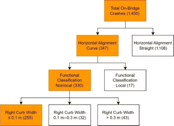
- Identify focus facility-type(s): Focus facility-types are those facilities where the focus crash-type is occurring. This can be identified based on prevalence or overrepresentation. As shown in Figure 4, a crash tree can be a useful tool to visualize the distribution of focus crashes and identify focus facility-types. In this guide, the focus facility-types include all facility types. It was difficult to determine overrepresented facility types because only a portion of BrTS crashes could be linked to corresponding bridges or tunnels. As BrTS crash and roadway data improve, agencies could consider the functional classification of the on-bridge or under-bridge roadways or designated truck routes to define the focus facility-type(s).
- Identify risk factors: Risk factors are characteristics associated with an increased risk of the focus crash-type occurring on the focus facility-type. The term “risk” has a wide range of definitions, but in this guide, it serves as a measure of two components: (1) the likelihood of a BrTS crash, and (2) the consequences of a BrTS crash should one occur. Risk factors can range from site-specific characteristics (e.g., bridge and roadway features) to area-wide characteristics (e.g., driver population, vehicle fleet, state policies). Risk factors do not necessarily reflect causal relationships. Instead, risk factors are “associated with” an increased likelihood or consequence of BrTS crashes. In a risk-based assessment, agencies can use risk factors to prioritize locations for further investigation and potential improvements.
A risk-based approach has several benefits that include the following abilities:
- Identify high-risk locations that may or may not have a high-crash history: One of the primary benefits of the risk-based approach is that agencies do not have to wait for crashes to occur to address potential issues. The risk-based approach allows agencies to identify locations with a high risk of a BrTS based on network, corridor, and site characteristics. Agencies can then proactively implement strategies to address the risk factors rather than waiting for crashes to occur.
- Overcome data limitations: For less common crash types, including BrTS crashes, the risk-based approach is particularly well suited to overcome data limitations, such as small sample sizes and limited information on exposure measures. Related to sample size, there are often relatively few reported BrTS crashes at any given location. Related to exposure, there may be limited data on the number or proportion of trucks and oversize vehicles to help predict BrTS risk. The risk-based approach overcomes these limitations by incorporating other characteristics, such as bridge and tunnel characteristics, general roadway and operational characteristics, and land use and policy data to proactively assess risk in the absence of high numbers of crashes.
- Address regression-to-the-mean: Regression-to-the-mean is the seemingly random fluctuation in crashes from year to year. On average, a given location has a long-term average number of crashes, but the observed number of crashes in a given year will generally be higher or lower than that average. Regression-to-the-mean explains how a location with multiple crashes one year may, without any intervention, experience below- or above-average crashes in subsequent years. For instance, the average number of BrTS crashes at a specific bridge is usually zero but may vary over time. Despite this variability in observed crashes year to year, the risk of a crash occurring is still present, and this risk is higher at some locations based on site-specific characteristics. While historical crash data may not identify these locations as a high priority, the risk-based approach can help to identify sites with high risk.
The next section describes common BrTS risk factors and the scenarios in which the risk factors are most relevant.
2.2 Common BrTS Risk Factors
Agencies can use a wide range of data to identify risk factors. Categorically, risk factor data can include the following:
- Operational data: traffic volume, truck and bus volume, lane use, signing, and markings.
- Geographic and contextual data: State- and agency-level policies, adjacent land use, and trip generators (e.g., industrial parks, distribution centers, fabricating facilities, storage yards).
- Crash data: historical crash frequency from police crash reports or transportation agency–maintained BrTS reports.
- Roadway infrastructure data: geometric alignment, cross section, and proximity to ramps.
- Bridge infrastructure data: presence, location, dimension, and condition of bridges, tunnels, and barriers.
The project team generated a list of potential risk factors pertinent to on-bridge and under-bridge BrTS crashes. Table 2 shows the variables that were considered and assessed as potential risk factors. Note that Table 2 presents various types of potential risk factors: (1) binary (e.g., yes/no or present/not present indicator), (2) categorical (e.g., number of lanes, type of lighting, shoulder width), and (3) continuous (e.g., traffic volume, bridge age, bridge length). Additional analysis will identify which variables appear as risk factors for different types of BrTS crashes and, for categorical and continuous variables, which categories or ranges are associated with an increased risk. While other research studies have identified additional variables as potential risk factors in BrTS crashes, the variables below are those that are readily available for further analysis. Section 2.4 describes analysis procedures if agencies have more detailed information and are interested in assessing risk factors such as state- or jurisdiction-level operations data. For instance, the proximity of a bridge to the nearest access point on a controlled access facility (e.g., first bridge versus subsequent bridges) is likely a risk factor in BrTS; however, these data are not readily available in current datasets. There is an opportunity for future research to collect and analyze these types of additional risk factors for consideration in the identification of high-risk locations and potential mitigation.
Table 3 provides a summary of confirmed risk factors by focus crash-type. The research team developed statistical models, as described in Section 2.4, to assess and confirm the risk factors. As described previously, this guide does not include specific focus facility-types for BrTS crashes. The research team considered roadway functional classification to define focus facility-types but determined it was more appropriate to include functional classification as a risk factor due to data limitations. While these risk factors are largely infrastructure-based, agencies could assess and apply additional factors such as state- or jurisdiction-level operational and educational policies and practices. Further, it is important to note that these factors are associated with higher risk and should not be interpreted as causal factors. In some cases, the results may seem counterintuitive. For instance, a larger deck width is associated with a higher risk of on-bridge strikes, while one of the countermeasures in Chapter 3 is enhanced lateral clearance. The relationships shown in the table may be confounded by other variables in the model or by omitted variables. These factors are simply used to identify higher-risk locations. Agencies should refer to Chapter 3 for further details on the expected safety effectiveness of specific countermeasures.
2.3 Applying Risk Factors to Prioritize Locations
The objective of this step is to use the risk factors to prioritize locations for further investigation and potential safety improvement. As shown in Figure 5, the process includes identifying locations for screening, calculating a risk score for each location, and prioritizing the locations based on the total risk score.
Table 2. Potential risk factors for BrTS.
| Bridge or Roadway Features | Description | On-Bridge | Under-Bridge or Tunnel Entrance |
|---|---|---|---|
| AADT | Annual average daily traffic | • | • |
| Approach rail (Y/N) | Presence of guardrail on approach | • | — |
| Approach rail end (Y/N) | Presence of guardrail end on approach | • | — |
| Approach roadway width | Width of usable roadway approaching bridge | • | — |
| Average shoulder width | Average shoulder width of roadway | • | • |
| Bridge age | Bridge age | • | • |
| Bridge length | Bridge length | • | • |
| Bridge serviceability and functional obsolescence | Bridge serviceability and functional obsolescence | • | • |
| Bypass, detour length | Bypass, detour length for roadway | • | • |
| Curb (Y/N) | Presence of curb on roadway | • | • |
| Curb width | Curb width | • | • |
| Curve (degree) | Degree of horizontal curve of roadway | • | • |
| Curve (k-value) | k-value of vertical curve of roadway | — | • |
| Curve length | Length of curve | • | • |
| Deck condition rating | Condition rating of bridge deck | • | • |
| Deck width | Deck width | • | • |
| Flare (Y/N) | Presence of flare (variable width of structure) | • | — |
| Functional classification | Functional classification of roadway | • | • |
| Horizontal clearance | Total horizontal clearance for roadway | • | • |
| Lateral clearance | Lateral clearance | • | • |
| Lighting | Type of lighting present on roadway | • | • |
| Maximum span | Length of maximum span of bridge | • | • |
| Median width | Width of median grass or sod | • | • |
| Narrow approach (Y/N) | Indicator for structure narrower than approach | • | — |
| National truck network | Indicator if roadway is part of national truck network | • | • |
| Number of lanes | Total number of lanes on roadway | • | • |
| Operation (1-way/2-way) | Direction of traffic (1 -way/2-way) on roadway | • | • |
| Paved road (Y/N) | Presence of paved road | • | • |
| Railing (Y/N) | Presence of railings on bridge | • | — |
| Roadway width | Width of roadway | • | • |
| Rumble strip (Y/N) | Presence of longitudinal rumble strips | • | • |
| Shoulder type | Pavement type of shoulders on roadway | • | • |
| Speed limit | Speed limit of roadway | • | • |
| Surface type | Pavement type of lanes on bridge | • | • |
| Transition (Y/N) | Presence of transition rails | • | — |
| Truck AADT | Truck annual average daily traffic | • | • |
| Truck percentage | Percentage of truck traffic | • | • |
| Variable vertical clearance | Vertical clearance varies by lane | • | • |
| Vertical clearance | Vertical clearance over roadway | • | • |
Note: — = Not a risk factor.
Table 3. Summary of confirmed risk factors for BrTS focus crash-types.
| Category | Variable/Risk Factors | On-Bridge Strikes (e.g., truss, parapet, railing) | Under-Bridge Strikes with Overhead Structure (e.g., girder) or Tunnel Entrance | Under-Bridge Strikes with Pier or Support (e.g., bent, support, pier, abutment) or Tunnel Entrance |
|---|---|---|---|---|
| Exposure | One-way traffic/dual carriage | • | — | • |
| Larger AADT | • | • | • | |
| Larger truck AADT | • | • | • | |
| More than two travel lanes | — | • | • | |
| Part of national truck network | — | — | • | |
| Rural arterial | • | — | — | |
| Rural local | — | — | • | |
| Rural major collector | • | — | — | |
| Rural minor collector | • | — | — | |
| Urban local | — | • | • | |
| Urban minor arterial | — | — | • | |
| Urban other principal arterial | — | — | • | |
| Design | Concrete shoulder | — | — | • |
| Concrete surface | — | — | • | |
| Curve (larger degree) | — | — | • | |
| Larger bridge roadway width | • | — | — | |
| Larger deck width | • | — | — | |
| Larger lateral clearance | — | • | — | |
| Longer bridge length | • | — | — | |
| Lower vertical clearance | — | • | — | |
| Approach road narrower than bridge | • | — | — | |
| No transition from road to bridge | • | — | — | |
| Presence of longitudinal rumble strip | — | — | • | |
| Presence of railing on bridge | • | — | — | |
| Presence of guardrail on approach | • | — | — | |
| Structure flared | • | — | • | |
| Unpaved road | • | — | — | |
| Condition | Lower deck condition rating | • | — | — |
| Older bridge | • | • | — |
Note: — = Not a risk factor.
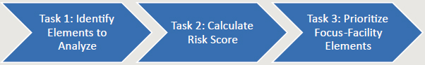
Table 4. Example element table for bridges and on-bridge roadways.
| Bridge Characteristics | On-Bridge Roadway Characteristics | ||||||||
|---|---|---|---|---|---|---|---|---|---|
| Bridge ID | Age (year) | Max. Span Length (m) | Serviceability/Functional Obsolescence | Crash Count in 5 Years | Functional Classification | AADT | % Trucks | # Lanes | National Network for Truck |
| 1830210 | 64 | 16.7 | 0 | 7 | Urban – Principal Arterial – Interstate | 43,750 | 16 | 3 | Yes |
| 1910363 | 11 | 35.9 | 29 | 4 | Urban – Principal Arterial – Other Freeways or Expressways | 13,500 | 12 | 2 | No |
| 1970057 | 5 | 10.3 | 17 | 4 | Rural – Minor Collector | 1,200 | 6 | 2 | No |
| 810221 | 56 | 16.4 | 22 | 3 | Urban – Collector | 2,100 | 7 | 2 | No |
The screening and prioritization process requires an integrated dataset, including the focus facility-types and the features associated with each location (e.g., bridge, tunnel, roadway, operational, and policy characteristics) to produce a risk score. The recommended practice for integrating and preparing the data for this step is to use spatial or tabular data tools, such as geographic information systems (GIS) or spreadsheets. The spatial data capabilities in GIS tools provide additional opportunities for agencies to integrate various sources of spatial and tabular data for risk-based scoring.
Task 1 – Identify Elements to Analyze
In this task, agencies identify the elements of interest (e.g., bridges, tunnels, roadways) from the focus facility-type. There are various options for this task. For instance, this could include all bridges and all tunnels on all facility types across the network. An agency may also choose to focus on a more select list, such as only bridges or only tunnels on one or more focus facility-types across the network depending on the intent of the analysis and potential funding program.
Table 4 is a sample of elements of interest for bridges and on-bridge roadways. Table 5 is a sample of elements of interest for bridges and under-bridge roadways. As shown in the tables,
Table 5. Example element table for bridges and under-bridge roadways.
| Bridge Characteristics | Under-Bridge Roadway Characteristics | ||||||||
|---|---|---|---|---|---|---|---|---|---|
| Bridge ID | Age (year) | Max. Span Length (m) | Crash Count in 5-years | Functional Classification | AADT | % Trucks | # Lanes | Min. Vertical Clearance (m) | National Network for Truck |
| 630280 | 42 | 20.4 | 12 | Urban – Local | 11,000 | 12 | 2 | 3.74 | No |
| 670265 | 59 | 19.8 | 2 | Urban – Collector | 38,500 | 12 | 4 | 4.49 | Yes |
| 510129 | 4 | 28.0 | 1 | Urban – Principal Arterial – Other Freeways or Expressways | 3,500 | 6 | 2 | 4.81 | No |
each location (row) should have the features associated with each risk factor (column). Agencies can use spreadsheets, GIS, and other tools to integrate data. Spreadsheets are useful for organizing the elements in tabular format and collecting relevant uniform data in each column. GIS offers more sophisticated analysis options to create and analyze elements, including the ability to incorporate spatial data such as state-level policies and regulations, jurisdiction-level operation practices, or proximity to carriers with low safety ratings.
Task 2 – Calculate Risk Score
This task involves calculating the risk score for each element (i.e., for each row in Tables 4 and 5). In this context, “risk score” is a quantitative measure based on the presence and weight of risk factors for the element. The risk score is ultimately used for prioritizing the elements.
There are two primary options for computing the risk score:
- Binary risk factor score and
- Regression-based risk factor score.
All agencies have access to the National Bridge Inventory (NBI) and National Tunnel Inventory (NTI); these are national datasets of bridge, traffic, and roadway characteristics that served as the basis for the regression-based risk factor modeling in this guide. As such, all agencies have the basic data required to compute risk scores using the regression-based risk factor method. If an agency would like to include additional risk factors in the scoring process (e.g., operational policies and practices), then the binary risk factor scoring method might be more applicable, especially for the additional factors.
Binary Risk Factor Score
One option is to assign a binary score (0 or 1), using 1 to indicate the presence or 0 to indicate the absence of each risk factor and prioritize locations based on the risk score. Using this approach, locations with the most risk factors would be ranked as the highest priority. Table 6 provides an example prioritization using this binary approach for functional classification, year built, minimum vertical clearance, and national truck network. In this example, the presence of a risk factor is simply flagged with a 1 and the absence of a risk factor with a 0 (shown in parentheses after the actual value for the variable). The risk factor scores are summed across each row to calculate the risk score for each site as shown in the final column.
Based on the example in Table 6, it is clear that one or more sites may receive the same risk score. This can create challenges when an agency is prioritizing a large number of sites. To overcome this issue, an agency can apply weights to one or more of the risk factors (e.g., 0.25, 0.5, 1.0, 2.0) depending on the relative importance of each factor. Analysts can use the overrepresentation charts to guide the weighting decisions where variables that appear to be more overrepresented
Table 6. Example prioritization table for bridges and tunnels on focus facility.
| Bridge ID | Crash Count | AADT | Functional Classification | Year Built | Minimum Vertical Clearance | National Network for Truck | Total Risk Score |
|---|---|---|---|---|---|---|---|
| B400047 | 24 | 1,800 | Urban Local (1) | 1959 (1) | 12’4” (1) | 1 (1) | 4 |
| B400271 | 4 | 200 | Urban Local (1) | 1966 (1) | 12’4” (1) | 0 (0) | 3 |
| B640031 | 2 | 21,600 | Rural Principal Arterial – Other (0) | 1967 (1) | 14’9” (0) | 0 (0) | 1 |
| B050147 | 1 | 4,400 | Urban Local (1) | 1974 (0) | 14’7” (0) | 0 (0) | 1 |
| B400916 | 0 | 3,400 | Urban Minor Arterial (0) | 2016 (0) | 20’11” (0) | 0 (0) | 0 |
could be weighted higher than variables that are only slightly overrepresented. This can introduce subjectivity into the process but provides flexibility in how an agency considers each factor in the prioritization process. The next section describes a more rigorous process for assigning variable weights.
Regression-Based Risk Factor Score
Another option is to use a statistical model to predict the likelihood of a crash and then use the model prediction as the risk score to prioritize locations. In this approach, an agency would use the statistical model to weight each factor; however, rather than using subjective weights, the coefficients estimated during the modeling process serve as weights for each risk factor.
The industry standard for predictive crash modeling is a negative binomial (NB) crash count model. Using these models, agencies can estimate the number of BrTS crashes at a given location based on the site-specific characteristics.
The following is the general formulation of the equation to predict BrTS crashes.
where
- BrTS Crashesi = the estimated bridge strikes at bridge i;
- n = the number of years considered for the study (e.g., 5 years);
-
Structure Length = the length of the structure defined as:
- Length of bridge structure for on-bridge strikes (e.g., truss, parapet, railing),
- Length of deck for both under-bridge strikes with overhead structure (e.g., girder) and under-bridge strikes with pier or support (e.g., bent, support, pier, abutment);
- AADT = the annual average daily traffic (based on the type of the estimated crash);
- xij = the quantitative measure of each explanatory variable j associated with bridge i;
- α and βj = estimated model coefficients for the explanatory variable q; and
- β0 = the estimated constant.
Task 3 – Prioritize Elements
The objective of this task is to prioritize the elements based on the risk scores and other potential factors as desired. The task begins with a simple ranking—rank the elements from the highest risk score to the lowest. Agencies can set thresholds for priority elements to help focus on a manageable number of bridges or tunnels. Agencies can create visualizations in addition to simple ranked lists. Figure 6 is an example of how an agency could visualize high-, medium-, and low-risk locations. Again, GIS tools are useful for visualizations and spatial analysis.
In some cases, an agency may want to prioritize a single list of elements that are scored using different risk factor criteria. For instance, one set of elements (e.g., bridges) may be scored from a total of nine risk factors, and another set of elements (e.g., tunnels) may be scored from a set of seven risk factors. In these cases, it is appropriate to normalize the risk scores to facilitate comparison across the different elements (e.g., bridges versus tunnels). To create normalized risk scores, agencies can divide the assigned risk score by the total potential risk score. The agency can then prioritize the various elements using the normalized risk score.
Table 7 shows an example with several elements that are first scored using three different sets of risk factor criteria and then normalized by the maximum possible risk score to prioritize across all elements in a single list. For example, Site 1 received an initial risk score of 6 out of a maximum possible risk score of 7. The normalized risk score for Site 1 is 0.86 (i.e., 6/7).

Table 7. Example risk scores with normalization.
| Site ID | Risk Score | Maximum Possible Risk Score | Normalized Risk Score | Priority Rank |
|---|---|---|---|---|
| 1 | 6 | 7 | 0.86 | 3 |
| 2 | 1 | 7 | 0.14 | 7 |
| 3 | 4 | 7 | 0.57 | 4 |
| 4 | 8 | 8 | 1.00 | 1 |
| 5 | 7 | 8 | 0.88 | 2 |
| 6 | 5 | 9 | 0.56 | 5 |
| 7 | 2 | 9 | 0.22 | 6 |
In other cases, an agency may want to include other factors to prioritize elements that represent substantial consequences should a crash occur. Substantial consequences could include conditions where a BrTS would close down a road that serves a hospital, emergency response (e.g., fire or police station), school, a high-traffic-volume roadway, or a roadway without an alternative route. At this stage, the consequences can further be applied to prioritize elements and serve as a tiebreaker for locations that have approximately the same likelihood of a crash occurring. For instance, if the following two locations have an equal risk score, which one would take priority?
- Rural, two-lane road that serves 500 vehicles per day and a residential community with alternate access available.
- Urban, six-lane arterial that serves 25,000 vehicles per day and a nearby hospital.
The BrTS crash at the second location would likely have more severe community and operational impacts if a crash occurred. As such, an agency may prioritize this location for further review and improvement.
2.4 Analyzing Data to Identify Risk Factors
This section focuses on data analysis to help practitioners and researchers replicate the results from this study with more focused local data if desired. The first subsection describes the data needs, and the second subsection describes the analysis procedures. Data limitations should not be viewed as an impediment to a proactive risk-based analysis. At a minimum, states should be able to use existing crash data and information from the NBI and NTI for analysis. For agencies with limited data capabilities, there is an opportunity to collect and organize the data in a standard format to support a future risk-based program (refer to Section 2.5, “Collecting and Integrating Risk Factor Data”).
Data Needs
Data needs vary significantly based on the desired level of effort and analysis. At a minimum, agencies should have BrTS crash data. Ideally, these crashes are geolocated and integrated with infrastructure and traffic data, so an analyst can connect the existing infrastructure and traffic conditions to each crash.
The ideal dataset for this step includes the following data integrated at the crash- and site-level:
- Crash data, including crash type, vehicle type, truck classification, OS/OW hauling permit, severity, location, and contributing factors.
- Roadway data, including cross section, geometry, and grade for the on-bridge, under-bridge, and tunnel roadways.
- Bridge and/or tunnel data, including physical characteristics of the bridges and tunnels. Agencies can download bridge and tunnel data from the NBI and NTI, respectively.
- Traffic volume data, including traffic volume, truck volume (or percentage trucks), and number of oversize loads.
- Supplemental data, including state or local policies, land use data, warning signs and systems, and asset management inventories (e.g., sign inventories).
Refer to Section 2.5, “Collecting and Integrating Risk Factor Data,” for further details on how to collect, process, and integrate these data. The section also provides sample templates to illustrate the appropriate data format.
Analysis Procedures
There are three general quantitative approaches to identifying and mitigating risk factors:
- Critical event analysis,
- Overrepresentation, and
- Statistical modeling.
Critical event analysis is a site-specific analysis approach that involves a detailed review of crashes and the context of the specific location to identify the plausible sequence of events leading up to a crash. Overrepresentation is a basic system-level analysis approach that offers an option for agencies with limited data or analysis capabilities. Statistical modeling is an advanced system-level analysis approach that requires a certain level of data and expertise to perform but can offer more insightful results.
Agencies can select the preferred approach based on the context of the analysis (site versus system), data capabilities, and resources available to perform the analysis. The following sections describe each approach with example applications.
Option 1: Critical Event Analysis—A Site-Specific Analysis Approach
Critical event analysis is a site-specific analysis approach agencies can use to identify risk factors. In this approach, agencies perform a detailed review of historical crashes (if applicable) and examine the context of the specific location (e.g., location of ramps, placement of signing, and availability of turnarounds and alternative routes) to identify the plausible sequence of events leading up to a crash. The idea is that there are generally multiple events (or contributing factors) that lead to a crash. Once an agency identifies and understands these events, it can mitigate crash risk by removing one or more of the events (factors). This is similar to the root cause analysis performed by the National Transportation Safety Board for major crashes or the failure mode and effects analysis (FMEA) performed by the National Aeronautics and Space Administration for major incidents. In the FMEA, “failure mode” is an event that increases the risk of an incident. “Event analysis” is an assessment of the consequence of a particular failure mode (e.g., what is the contribution of a specific factor to the overall risk of an incident).
For a more systematic approach, agencies could develop a checklist to assist bridge and tunnel engineers in identifying locations or factors that are at a higher risk of a BrTS. Similarly, industry organizations and motor carriers can develop checklists to assist drivers in identifying factors related to the load (e.g., height, width, and load securement) that increase the risk of a BrTS. Refer to Section 3.3 for further details on checklists.
Critical Event Analysis: Example Application
In this example, critical event analysis is used to postulate the sequence of events leading to a BrTS classified as an under-bridge collision with the superstructure. The analysis is based on one historical crash and the context of the specific bridge. The crash involved an OHV compared to the bridge height. The driver had a permit but deviated from the designated route. Based on the police officer’s narrative, the driver was unfamiliar with the area and was looking to correct course. Based on the crash data, it was dark when the crash occurred. Based on a site review during the day, there were warning signs well in advance of the bridge to indicate the low-clearance height. Based on a site review at night, it became evident that the advance warning sign was worn and difficult to see. Figure 7 shows a potential sequence of events to better understand the contributing factors and opportunities to mitigate BrTS risk for this specific scenario.
There is an opportunity to mitigate BrTS risk at this location by eliminating one or more factors from the sequence of events. For instance, if the driver was familiar with the area, then they would have remained on the designated route. If the driver was transporting the load during the day or if the warning signs were more conspicuous, then the driver may have stopped before the bridge. If the bridge was designed to standard height clearance, then the load would not be considered overheight. The crash may have been avoided if just one factor had been removed from the scenario. Of course, some of the factors are more expensive to address than others, and addressing multiple factors adds redundancy.
Option 2: Overrepresentation—A Basic System-Level Approach
Overrepresentation is a basic system-level approach agencies can use to identify risk factors. In this approach, agencies compare the proportion of BrTS crashes at locations with given attributes to the proportion of an exposure measure, such as the number of sites or vehicles passing through those locations.
Overrepresentation: Example Application
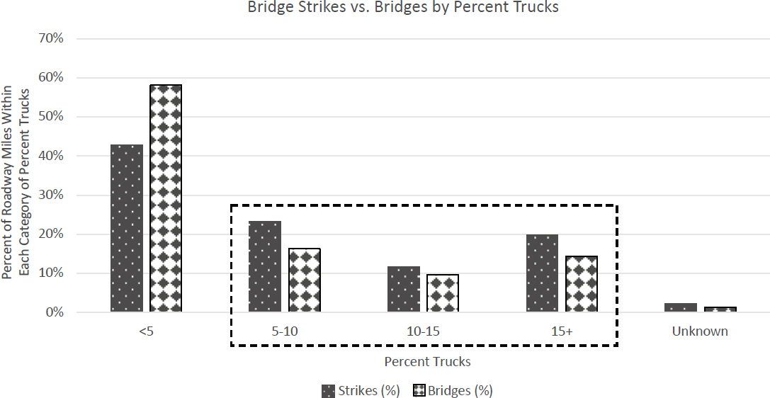
In this example, overrepresentation analysis is used to assess five categories of percent trucks as BrTS risk factors within a defined geographic area (e.g., a region or state). Specifically, the analysis compares the percentage of BrTS associated with each category of percent trucks to the percentage of bridges associated with the same category. As shown in Figure 8, it is easy to identify those categories that stand out as risk factors. In this case, the proportion of BrTS crashes is greater than the proportion of bridges for the 5–10, 10–15, and 15+ categories. These overrepresented categories indicate that truck percentage greater than 5% is a risk factor for this example.
Option 3: Statistical Modeling—A More Rigorous System-Leven Approach
Statistical modeling is a more rigorous system-level approach agencies can use to identify risk factors. In this option, agencies use their own data to develop crash frequency or crash probability regression models for BrTS crashes on one or more focus facility-types. The regression model uncovers features that are statistically correlated with increased frequency or probability of BrTS crashes, depending on the model type. Each variable in the model can be considered a risk factor.

Agencies can use the model results as described in the earlier Section, “Task 2 – Calculate Risk Score,” to prioritize locations based on predicted risk.
Statistical Modeling: Example Application
In this example, an agency developed a statistical model to assess several variables as risk factors for under-bridge strikes with overhead structures. Table 8 summarizes the model results, which were estimated using NB regression. As shown in the table, each of the variables is associated with an increase in the likelihood of an under-bridge strike with an overhead structure. This is evident from the column, Estimates (i.e., all positive coefficients). As such, all of these variables could be identified as risk factors for under-bridge strikes with an overhead structure.
Table 8. Summary of regression model for under-bridge strikes with an overhead structure (e.g., girder).
| Parameter | Estimate | Standard Error | Pr > z |
|---|---|---|---|
|
(Intercept) |
0.7622 | −8.0140 | — |
|
Log of Under-Bridge Average Daily Traffic |
0.0779 | 3.8390 | 0.00 |
|
Bridge Age |
0.0048 | 3.2270 | 0.00 |
|
Functional Classification of Under-Bridge Roadway: Rural Interstate |
0.3123 | −3.3610 | 0.00 |
|
Functional Classification of Under-Bridge Roadway: Urban Interstate |
0.2871 | −1.6660 | 0.10 |
|
Functional Classification of Under-Bridge Roadway: Urban Other Principal Arterial |
0.2528 | 2.6110 | 0.01 |
|
Functional Classification of Under-Bridge Roadway: Urban Local |
0.2491 | 8.0790 | 0.00 |
|
Length of Maximum Span of the Bridge |
0.0103 | −4.7450 | 0.00 |
|
Average Daily Truck Traffic Percentage of Under-Bridge Roadway |
0.0190 | 3.3110 | 0.00 |
|
Number of Lanes Under Bridge |
0.0536 | 2.1680 | 0.03 |
|
Bridge Serviceability and Functional Obsolescence |
0.0106 | −1.7690 | 0.08 |
The standard error is used in combination with the estimate to determine the statistical significance of the variable, which is expressed in the final column of the table (Pr > z). A value less than 0.10 indicates the variable is statistically significant at the 90% confidence level; a value less than 0.05 indicates the variable is statistically significant at the 95% confidence level. In this example, all variables are statistically significant at the 90% confidence level or higher.
This example shows the wide range of features that can be considered as BrTS risk factors using statistical modeling. Agencies should consult previous studies and literature, including the results of this research, when identifying potential risk factors for a risk-based analysis.
2.5 Collecting and Integrating Risk Factor Data
This section focuses on data collection and integration procedures to support BrTS risk assessments, beginning with details on processing existing state-level data (state-maintained crash data) and national-level data (NBI and NTI). It describes two methods for linking crash data to specific bridges or tunnels, along with the challenges and opportunities to overcome those challenges. The section concludes with a discussion of how agencies can contribute to the BrTS Clearinghouse for collecting and analyzing BrTS data and communicating bridge and tunnel clearance information. By collecting and integrating additional data elements, agencies will be able to perform more robust and reliable risk assessments to mitigate BrTS risk. By updating the Clearinghouse with more complete and reliable data, agencies will support more advanced and automated risk-based screening and prioritization. The Clearinghouse will also serve as a means to communicate bridge and tunnel clearance information, which is one of the most important factors in mitigating BrTS risk.
Crash Data
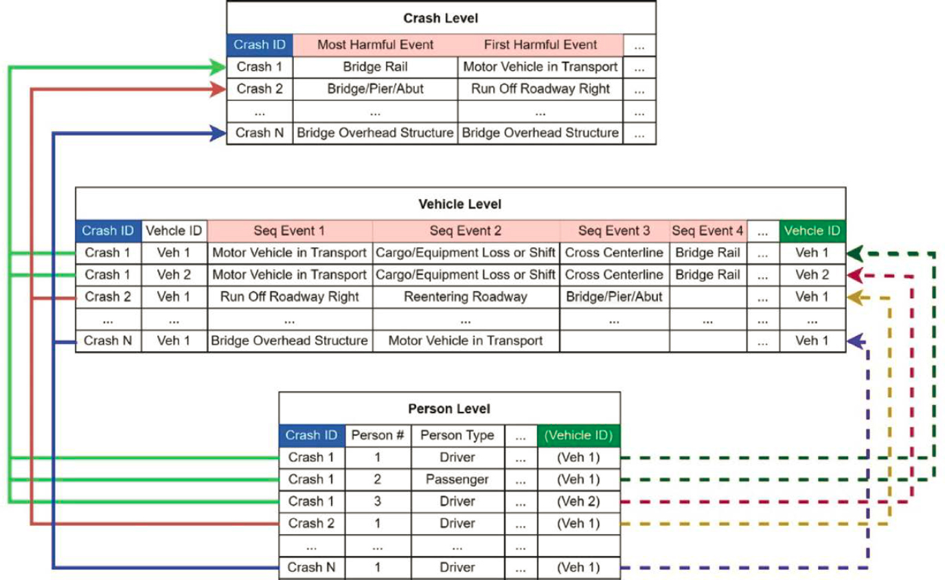
Although a BrTS is defined as a collision between a motor vehicle and a bridge or tunnel, the actual query of such information is not straightforward since there are various ways to store and present the information. The relational crash database in Figure 9 illustrates the recommended method for querying a BrTS. As shown, events related to bridge strikes can be archived at the vehicle level or crash level. Vehicle-level data elements describe the characteristics of the vehicles involved, while the crash-level data elements describe the overall characteristics of the crash. In most states, only the “most harmful event” and sometimes the “first harmful event” are available at the crash level. [“Most harmful event” is one that results in the most severe injury or, if no injury, the greatest property damage involving the motor vehicle. A “first harmful event” is defined as the first injury- or damage-producing event that characterizes the crash type (NHTSA 2017).] For these states, querying the most harmful events for bridge-related collisions will leave out a substantial number of bridge hits that are neither the most harmful nor the first harmful event. Therefore, agencies should query BrTS from data fields such as first harmful event (crash level), most harmful event (crash level), or sequence of events (vehicle level) for attributes such as “Bridge Overhead Structure,” “Bridge Pier or Support,” “Bridge Rail,” and “Other Fixed Object (wall, building, tunnel, etc.)” to compile a more complete dataset.
Ideally, the crash data should contain information to identify the specific bridge (based on a unique bridge ID) that can help specify which bridge parts were struck and distinguish bridge hits from tunnel hits. A few states do not distinguish by bridge part. For instance, the bridge-hit records from one state were all labeled as “Bridge Railing” crashes. In terms of tunnel strikes, very few states (e.g., Washington) assign dedicated attributes or fields to tunnels in the crash data. In general, the only way to identify tunnel hits from “Other Fixed Object (wall, building, tunnel, etc.)” or to identify a specific part of the bridge is to review the crash narrative. However, the
crash narrative is one of the data items that is frequently not available through data requests, and there are challenges in consistently querying the narrative for relevant information.
As states move toward all electronic crash reporting and compliance with the suggested data fields in the Model Minimum Uniform Crash Criteria (MMUCC), there will be more uniformity and consistency for identifying BrTS from the crash data. There will also be an opportunity to capture more details for each BrTS if the structure of the electronic crash form asks questions in a sequential order with logic to trigger additional questions as appropriate. In the interim, agencies can convert or collapse state-specific data fields and attributes to better align with MMUCC data fields. Table 9 shows an example of converting and collapsing the state-specific sequence of events field to the corresponding MMUCC attributes.
Table 9. Example of data fields/attributes conversion (Wisconsin).
| State Crash Data Field | MMUCC-Compliant Data Field |
|---|---|
| ANM DA – Domesticated Animal – Alive | Animal (live) |
| ANM NA – Non–Domesticated Animal (Alive) | Animal (live) |
| ANM DD – Domesticated Animal – Dead | — |
| ANM ND – Non–Domesticated Animal (Dead) | — |
| BRIDGE – Bridge Overhead Structure | Bridge Overhead Structure |
| BRPAR – Bridge Parapet End | — |
| BRRAIL – Bridge Rail | Bridge Rail |
| BRPIER – Bridge/Pier/Abut | Bridge Pier or Support |
| CABL B – Cable Barrier | Cable Barrier |
| CARGO – Cargo/Equipment Loss or Shift | Cargo/Equipment Loss or Shift |
| CONC B – Concrete Traffic Barrier | Concrete Traffic Barrier |
| CR CL – Cross Centerline | Cross Centerline |
| CR MED – Cross Median | Cross Median |
| CULVRT – Culvert | Culvert |
| CURB – Curb | Curb |
| DITCH – Ditch | Ditch |
| DOWN – Downhill Runaway | Downhill Runaway |
| EMBKMT – Embankment | Embankment |
| — | End Departure (T-intersection, dead-end, etc.) |
| EQP FL – Equipment Failure (Blown Tire, Brake Failure, etc.) | Equipment Failure (blown tire, brake failure, etc.) |
| FELL – Fell/Jumped from Motor Vehicle | Fell/Jumped from Motor Vehicle |
| FENCE – Fence | Fence |
| HYDRN – Fire Hydrant | — |
| FIRE – Fire/Explosion | Fire/Explosion |
| GR END – Guardrail End | Guardrail End Terminal |
| GR FAC – Guardrail Face | Guardrail Face |
| IMMER – Immersion, Full or Partial | Immersion, Full or Partial |
| ATTEN – Impact Attenuator/Crash Cushion | Impact Attenuator/Crash Cushion |
| JKNIF – Jackknife | Jackknife |
| LT TRN – Left Turn | — |
| LTPOLE – Lum Light Support | — |
| MAILBOX – Mailbox | Mailbox |
| MVIT – Motor Vehicle in Transport | Motor Vehicle in Transport |
| OT RDY – Motor Vehicle in Transport – Other Roadway | — |
| OTH FX – Other Fixed Object | Other Fixed Object (wall, building, tunnel, etc.) |
| OTH NC – Other Non-Collision | Other Non-Collision Harmful Event |
| State Crash Data Field | MMUCC-Compliant Data Field |
|---|---|
| OT NMT – Other Non-Motorist | Other Non-Motorist |
| OBNFX – Other Object – Not Fixed | Other Non-Fixed Object |
| — | Other Non-Harmful Event |
| OT PST – Other Post, Pole or Support | Other Post, Pole, or Support |
| THER B – Other Traffic Barrier | Other Traffic Barrier |
| OH PST – Overhead Sign Post | — |
| OVRTRN – Overturn/Rollover | Overturn/Rollover |
| PKVEH – Parked Motor Vehicle | Parked Motor Vehicle |
| BIKE – Pedalcycle | Pedalcycle |
| PED – Pedestrian | Pedestrian |
| TRAIN – Railway Vehicle (Train, Engine) | Railway Vehicle (train, engine) |
| REENTR – Reentering Roadway | Reentering Roadway |
| RT TRN – Right Turn | — |
| ROR L – Run Off Roadway Left | Ran Off Roadway Left |
| ROR R – Run Off Roadway Right | Ran Off Roadway Right |
| SEP – Separation of Units | Separation of Units |
| — | Strikes Object at Rest from MV in Transport |
| STRUCK – Struck by Falling, Shifting Cargo or Anything | Struck by Falling, Shifting Cargo or Anything |
| Set in Motion by Motor Vehicle | Set in Motion by Motor Vehicle |
| THRWN – Thrown or Falling Object | Thrown or Falling Object |
| SIN PST – Traffic Sign Post | Traffic Sign Support |
| TF SIG – Traffic Signal | Traffic Signal Support |
| TREE – Tree | Tree (standing) |
| UNKN – Unknown | Unknown Fixed Object |
| UT PL – Utility Pole | Utility Pole/Light Support |
| WZ EQP – Work Zone/Maintenance Equipment | Work Zone/Maintenance Equipment |
National Bridge Inventory and National Tunnel Inventory
The NBI database contains information for more than 615,000 bridges on public roads and publicly accessible bridges on federal and tribal lands. The NBI contains inventory and inspection information collected by state DOTs, federal agencies, and tribal governments. The bridge inventory and inspection data are categorized into the following seven sections:
- Bridge identification;
- Bridge material and type;
- Bridge geometry;
- Features;
- Loads, load rating, and posting;
- Inspections; and
- Bridge condition.
Similarly, the NTI is also a national database that contains information describing more than 500 tunnels on public roads, including interstates, U.S. highways, and state and county roads as well as publicly accessible tunnels on federal lands. The tunnel inventory data are categorized into the following eight sections:
- Identification,
- Age and service,
- Classification,
- Geometric data,
- Inspection,
- Load rating and posting,
- Navigation, and
- Structure type and material.
U.S. DOT Bureau of Transportation Statistics Railroad Bridge Data
The NBI includes very few railroad bridges. If an agency assigns bridge crashes to the nearest bridge without accounting for railroad bridges, then there is a higher chance of wrongful linkage. Specifically, there is a chance that a railroad bridge crash could be incorrectly assigned to a nearby highway bridge. Fortunately, the Bureau of Transportation Statistics (BTS) under the U.S. DOT compiled and published a railroad bridge database.
On October 14, 2022, BTS released the railroad bridge dataset from the Federal Railroad Administration and published it as part of the National Transportation Atlas Database. Based on the Code of Federal Regulations (49 CFR Part 237), a railroad bridge is defined as “any structure with a deck, regardless of length, which supports one or more railroad tracks, or any other under-grade structure with an individual span length of 10 feet or more located at such a depth that it is affected by live loads.”
While the railroad bridge dataset contains 69,510 railroad bridges, it includes very limited information on details such as ownership, structure, and traffic. Thus, the primary purpose of using this dataset is to locate railroad bridges and increase the accuracy of a spatial join between a crash and an NBI bridge. A “spatial join” is a fundamental operation within a GIS or spatial database, wherein it merges the attribute tables of two spatial layers, guided by a specified spatial relationship between their geometrical elements. In this case, it represents the merge between crash data and the NBI bridge inventory data. At a minimum, including this dataset can reduce the uncertainty of joining a crash with the wrong highway bridge in the NBI data.
Data Linkage
There are two primary methods to link crash and bridge data:
- Common ID and
- Spatial join.
Common ID
States can use the common ID linkage when the crash data contain a complete and accurate bridge ID that is the same ID found in the bridge inventory. This bridge ID is a universal unique identifier (UUID) for deterministic linkage between a crash record and the impacted bridge. For example, Maine’s bridge ID is a UUID in both the crash data and the bridge inventory. As such, Maine can directly link a BrTS to the impacted bridge. States are encouraged to enhance crash reporting practices and collect the bridge ID as part of the crash report. This will allow the use of the common ID linkage and improve the reliability of merging crash and bridge data. Refer to Section 2.5 for further discussion of opportunities to improve crash data collection for use in BrTS analysis and research.
Spatial Join
States can use the spatial join linkage when the structure ID is not available or not properly filled out in the crash data. The spatial join is a probabilistic linkage based on the Euclidean
distance (i.e., straight line distance as opposed to travel distance) between the crash location and bridge location. The accuracy of finding a correct match increases as the joined distance decreases.
The following are two primary issues related to the spatial join method given the location accuracy of both bridges and crashes.
- For states with a high bridge density, the clustering of bridges increases the likelihood of a crash being linked to the wrong bridge.
- There is a balance between accuracy and coverage of the spatial join depending on the location accuracy selected by the analyst. A short buffer distance (e.g., 50 feet) can increase the accuracy of the join but may result in many unlinked crashes. A longer buffer distance (e.g., 1,000 feet) may substantially increase the matches between crash records and bridges but may result in an incorrect linkage (e.g., crashes linked to multiple bridges or linked to the wrong bridge).
The most common spatial join method, called “closest join,” involves linking a crash to the nearest bridge. Another spatial join method, called “split join,” involves splitting a crash among bridges within some proximity. For the split join, agencies define a relevant distance and assign a fraction of a hit to each bridge within the distance rather than assigning 100% of a crash to the nearest bridge. If location data quality is a concern, split join may offset the impact of joining crashes to the wrong bridge.
Research conducted for this project assessed both crash assignment methods using data for Maine, North Carolina, and Wisconsin. Nine split joins were conducted: three for each state based on on-bridge strikes, under-bridge strikes, and under-bridge OHV strikes. Each bridge was assigned a fraction of a BrTS crash within 500 feet. The researchers then compared the linked results to the BrTS assigned by the closest join. The researchers used a paired t-test to determine whether the two samples were statistically different and a Fisher’s exact test to determine whether the two samples were independent. The paired t-test indicated that the two samples were statistically different, and the Fisher’s exact test showed that they were generally independent. This indicates that the method used to join BrTS crashes to bridges (closet join or split join) could impact the results of the analysis.
Based on this research, most crashes were within 500 feet of a bridge. When the crash was farther than 500 feet from a bridge, the accuracy of the spatial join deteriorated. Further, according to the descriptions in NBI, the latitude/longitude of a bridge generally refers to the beginning of a bridge in the direction of inventory. The average structure length of bridges in the NBI is approximately 150 feet, which suggests that for the majority of bridges, the 500-foot buffer covers the entire bridge length and its proximity.
To increase the accuracy of a spatial join, agencies should account for the missing railroad bridges in the NBI. To do so, agencies would first perform a spatial join between the crashes and railroad bridges and flag any potential railroad bridge-related crashes. This spatial join can be limited to under-bridge crashes only (i.e., overhead bridge structure strikes and the under-bridge strikes with pier or support) because a vehicle crash on a railway bridge is not expected. Based on the project team’s research, the difference between including and excluding railroad bridge crashes can be very large: 60% or more are flagged as railroad bridge hits. In Wisconsin, the percentage is even higher with more than 80% of crashes flagged as potential railroad bridge hits.
Tunnel strikes are identified as vehicle strikes within 1,500 feet of a tunnel. The buffer of 1,500 feet is set as the threshold because the national average tunnel length in the NTI is 1,300 feet. The location for a tunnel is set at its entrance.
National BrTS Data Clearinghouse
A national BrTS Clearinghouse is one opportunity to help overcome challenges in identifying, diagnosing, and mitigating BrTS risk. The following are keys to success.
- Keeping the structure inventory data up-to-date and in good quality: The NBI has missing, erroneous, and logically conflicting information (Dedman 2008; Dekelbab, Al-Wazeer, and Harris 2008; Din and Tang 2016) due to data entry errors. Similar issues afflict the NTI. As such, there is a need to work to improve the quality and timeliness of the underlying data.
- Establishing a reliable linkage between BrTS and structure inventory data: While crash, bridge, tunnel, and roadway databases contain valuable information, they are often in separate “silos” (i.e., collected and maintained by different departments or divisions). The MMUCC provides a mechanism to link bridge crashes with NBI data through a Bridge/Structure Identification Number (NHTSA 2017), but MMUCC compliance is optional and varies among states. Further, spatial joins can be subject to errors and should be validated before analysis. A BrTS Clearinghouse will help to establish these linkages.
- Extracting relevant data items from connected databases for collision risk analysis: The NBI, NTI, and crash databases each have multiple tables, numerous data elements, and thousands of records. The scale of the databases and the complex relationships among them make it challenging to extract useful information and to promptly make decisions regarding permits. The BrTS Clearinghouse will provide useful information for assessing risk based on the underlying data. It will also allow users to extract relevant data for more detailed analysis.
- Developing a rigorous approach to accurately calculate the collision risk and its outcome: Most state agencies, as part of their bridge (damage) inspection procedure, have methods for rating a bridge after the impact and policies for an efficient and effective response. Few have methods for proactively assessing bridges for the risk of being hit. The BrTS Clearinghouse will provide a method and results for assessing BrTS risk.
- Identifying and quantifying effective safety countermeasures for categories of BrTS: Quantifying the costs and benefits of targeted countermeasures will lead to more informed decisions on appropriate infrastructure and operational investments and strategies. Chapter 3 of this guide presents various countermeasures–from lower-cost signing and striping to higher-cost bridge improvements to state-level policy and operational procedures.
- Communicating highway structure conditions or concerns effectively among different stakeholders: Mitigating and avoiding BrTS require the cooperation of many stakeholders, including state and federal agencies, motor carriers, and private service providers. Effective communication and information exchange among different parties and agencies will lead to more effective BrTS programs, especially during permit issuance for OS/OW movements. This can also support improvements to the data availability and quality.
This section presents a BrTS Clearinghouse prototype for collecting and disseminating BrTS data along with a demonstration of how agencies could use it in practice. The goal is to create a sustainable national clearinghouse for states to collect and analyze BrTS data as well as communicate bridge and tunnel clearance information. While this section presents an initial prototype, there will be a need for future efforts, including a long-term storage plan and regular maintenance. For instance, there will be a need to update the data extract, transform, and load (ETL) processes as states change their crash and roadway databases. This section does not address these maintenance issues.
Prototype Design Concept
Figure 10 shows the conceptual design of the BrTS Clearinghouse. There are several components, including state crash records (left middle), NBI and NTI (top middle), and supplemental datasets (bottom middle). The result is a structured dataset with structure-based and crash-based
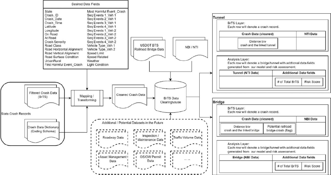
files (right). The figure shows the collection and processing of state crash records (left middle) as a three-step process:
- BrTS crash data requests are sent to state agencies. State agencies process existing state crash data to identify BrTS crashes that meet the inclusion criteria (i.e., crashes involving a strike to the bridge, tunnel, or its component parts).
- BrTS Clearinghouse maintenance staff transform the state BrTS crash data to meet the established standard data element definitions. This ensures the final database file and records have consistent definitions and formats. Records that fail to convert properly are examined and either corrected or excluded. The transformation process will be improved through an iterative process unique to each source file (state database).
- Each transformed and cleaned state BrTS crash file is added to the final file ready for analysis.
In parallel, the Clearinghouse retrieves structure data from NBI, NTI, and the U.S. DOT BTS railroad bridge dataset (top middle). The Clearinghouse integrates the structure data and crash data using either the common ID or spatial join method. If the structure ID is available in both the crash and structure data, then the common ID is used to join the data. If not, the spatial join is used based on available data (e.g., latitude/longitude, X/Y). The Clearinghouse could also incorporate additional data such as roadway characteristics, inspection and maintenance records, and traffic data (bottom middle).
The risk assessment module calculates basic statistics (e.g., number of crashes, injury severity, damage) for each bridge based on the embedded BrTS crash count models, injury severity models, and risk assessment method. The Clearinghouse creates a relational database for crash-based analysis and structure-based analysis. The flat file for crash-based analysis includes one record per BrTS crash. Table 10 shows an example of the resulting flat file. The flat file for structure-based analysis includes one record per bridge or tunnel.
At a minimum, the database will include the relevant crash data elements, the bridge or tunnel data elements, and any crucial metadata required for data management purposes. A visualization component could be developed via ArcGIS to produce corresponding layers for displaying related statistics (e.g., BrTS locations, number of BrTS for each bridge, flagged railroad bridge crashes, risk assessment score, etc.). Visualization tools could allow the user to toggle specific elements of interest such as bridge or tunnel groups or even different struck parts.
Prototype Demonstration
Fourteen states were selected to demonstrate the prototype based on the quality and completeness of crash data: Alaska, Arkansas, Connecticut, Florida, Illinois, Iowa, Maine, Mississippi, North Carolina, South Carolina, Tennessee, Utah, Washington, and Wisconsin. Specifically, these states have the essential data fields and attributes required for further analyses. The data from all 14 states can be used to identify certain bridge-related crashes. Typical situations regarding the bridge structure ID from the crash data can be categorized as the following:
- Crash data and corresponding NBI data have the same bridge ID, which can serve as the UUID for data linkage. Only Maine has such data.
- Crash data include one dedicated variable for recording the bridge ID, but a very small percentage of filled values are proper NBI bridge IDs (e.g., Wisconsin).
- Crash data do not include NBI bridge IDs, which is the most common case among the currently collected data from most of the states.
For tunnel-related crashes, there is rarely a direct linkage between the NTI data and the crash data from selected states as mentioned previously. Although NTI data are set up similarly to the NBI data with a specific tunnel structure ID, the crash data do not capture the tunnel ID.
Table 10. Prototype of the BrTS Data Clearinghouse flat file.
| State Crash Records | ||||||||||||
|---|---|---|---|---|---|---|---|---|---|---|---|---|
| Field Name | BrTS ID | State | Date | Time | Latitude | Longitude | On Road | At Road | … | |||
| Format | CHARa (50)b | CHAR(2) | DATE | TIME | NUM(10,8)c | NUM(10,8) | CHAR(50) | CHAR(50) | … | |||
| Description | ID in data clearinghouse | State postal abbreviation | Date of crash YYYY/MM/DD | Time of crash | Decimal degrees | Decimal degrees | Name of road on which crash occurred | Name of intersecting road to identify location | … | |||
| 1001 | WI | 2018/11/09 | 8:45 | 43.87680426 | −91.1832326 | THIRD | WALNUT | … | ||||
| 1002 | WI | 2020/10/02 | 13:20 | 44.08444452 | −87.7236331 | US 29 | SR 1619 | … | ||||
| 1003 | NV | 2013/03/06 | 7:50 | 40.06118260 | −118.6534580 | PEACE | GLENNWOOD | … | ||||
| 1004 | NV | 2013/05/25 | 21:10 | 40.80916510 | −115.8246880 | SUTTON | ARLINGTON | … | ||||
| 1005 | MA | 2019/02/04 | 17:05 | 42.59224383 | −71.2805723 | NC 226 | POTEAT | … | ||||
| 1006 | MA | 2019/02/12 | 9:02 | 41.94660778 | −71.2755011 | SALISBURY | OLD CHARLOTTE | … | ||||
| NBI/NTI | ||||||||||||
| Field Name | BrTS ID | Structure Number | Structure Material Structure Type | Minimum Vertical Clearance | Year Built | Detour Length | … | |||||
| Format | CHAR(50) | CHAR(50) | CHAR(50) CHAR(50) | NUM(3,2) | NUM(4,0) | NUM(3,0) | … | |||||
| Description | ID in data clearinghouse | Structure number/bridge identification number | Structure material | Type of structure design | Minimum vertical clearance (over-bridge roadway) or minimum vertical under-clearance (under-bridge roadway) in meters | Year the bridge was built | Kilometers | … | ||||
| 1001 | B32005400000000 | Steel continuous | Stringer/multibeam or girder | 4.84 | 1967 | 1 | … | |||||
| 1002 | B36006500000000 | Prestressed concrete continuous | Stringer/multibeam or girder | 4.65 | 1979 | 24 | … | |||||
| 1003 | B1040W | Concrete | Culvert | — | 1965 | 1 | … | |||||
| 1004 | I900W | Prestressed concrete | Box beam or girders – multiple | 5.00 | 1976 | 1 | … | |||||
| 1005 | B120062BBMUNNBI | Concrete | Arch – deck | — | 1950 | 2 | … | |||||
| 1006 | A160203YYDOT634 | Steel | Stringer/multibeam or girder | 5.70 | 1962 | 3 | … | |||||
aCHAR indicates a data type storing characters in a fixed-length field.
bNumbers in parentheses specify data length. A single number means no decimal portion.
cTwo numbers in parentheses also specify data length; the first is the number of integer digits, and the second is for decimal digits.
This subsection describes the procedures for the BrTS Clearinghouse prototype, along with challenges that can be addressed in future research. The current prototype is developed with the ArcGIS Online Application, which offers an interactive mapping interface to query and display crash and structure data and collision risk from the selected states. The development of the current version requires a certain level of manual effort to process the data.
Data Preparation
The first step is to obtain state BrTS crash data. Most states provided datasets to the research team using the given research team’s query requirements as previously described (i.e., most/first harmful event and sequence event). Some state systems, like Wisconsin’s WisTransportal, provide open access to data. In those cases, the research team used the same queries to obtain the data directly. The research team also queried the NBI, NTI, and railroad bridge datasets for the 14 selected states according to their state code. Geocoded data were transformed into decimal degrees for compatibility with ArcGIS.
Data Linkage
Maine’s data were linked by Common ID join, using the common bridge number in the NBI and the crash data. Some bridges were missing from the NBI data. In Wisconsin, even though some bridge numbers were provided, the structure number was typically inconsistent with the structure numbers available in the NBI data; therefore, a spatial join was conducted. Similarly, a spatial join was conducted for the other states, as there was no provision for bridge numbers. The spatial joins produced bridge-hit counts where repetitions of each structure number could be counted.
For states other than Maine, two spatial joins were conducted: one determined how many bridges were within a 100-foot buffer and one determined how many bridges were within a 500-foot buffer around each crash. Considering that NBI does not include most railroad bridges, the team utilized the railroad bridge dataset from the BTS website to flag potential railroad bridge-related crashes when a railroad bridge is the closest bridge within a 500-foot buffer of a given crash. Similarly, as mentioned previously, the buffer of 1,500 feet is set as the threshold for potential tunnel crashes to link with the tunnels because the national average tunnel length in the NTI is 1,300 feet. The location for a tunnel is set at its entrance.
Results and Presentations
The resulting prototype is a web application that aims to establish a national-level data repository for collecting and analyzing BrTS data.
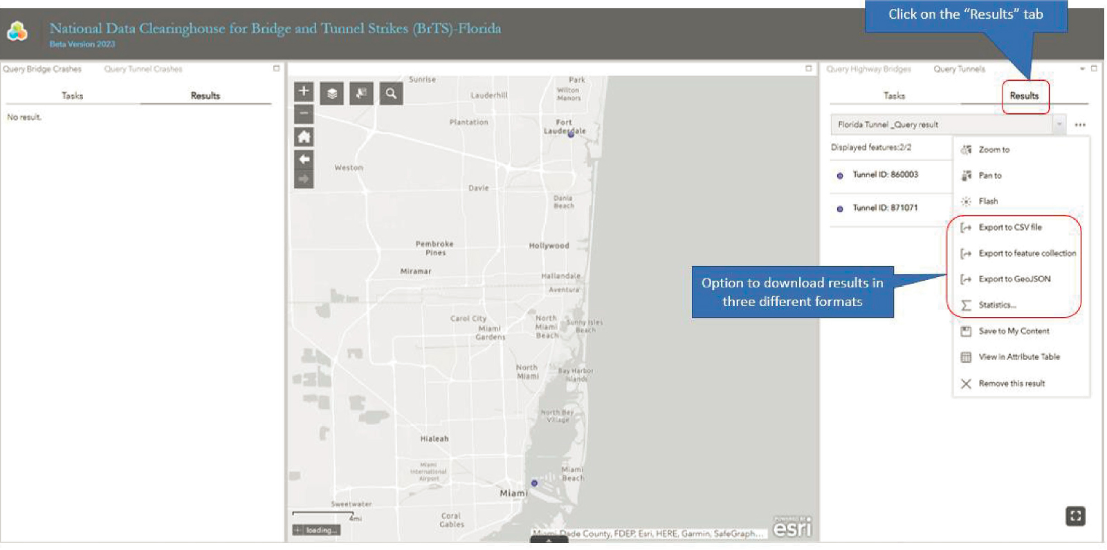
The BrTS Clearinghouse uses a data-driven method to assess BrTS risk. Transportation agencies and motor carriers can use this application to assess, quantify, and communicate the risk of bridge- and tunnel-related crashes. Refer to the subsection “Stagewise Data Clearinghouse Web Interface” for further details on how to view and query data. Notably, the functionalities listed in this guide are not exhaustive. Users can export the retrieved data to a comma-separated values (CSV) file, which is compatible with Microsoft Excel and ArcGIS.
Welcome Page.
Figure 11 shows the welcome page of the prototype tool. The welcome page provides links for the project information, the BrTS Clearinghouse, and the option to request data. This page also contains two links:
- “National Data Clearinghouse for Bridge and Tunnel Strikes (BrTS)” directs users to the project website that contains project information such as a general overview of the data clearinghouse, detailed information about the project, a user guide, and the option to request data.
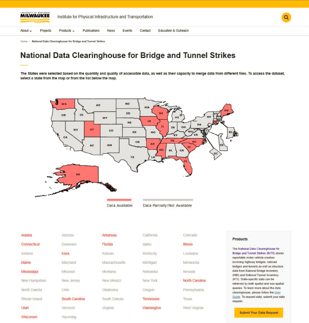
- “Submit Your Data Request” directs users to a data request form. The BrTS Clearinghouse stores data in an ArcGIS geodatabase where some data forms and fields may be modified or omitted from the original data due to the constraint of the geodatabase. For original data, users can submit a data request.
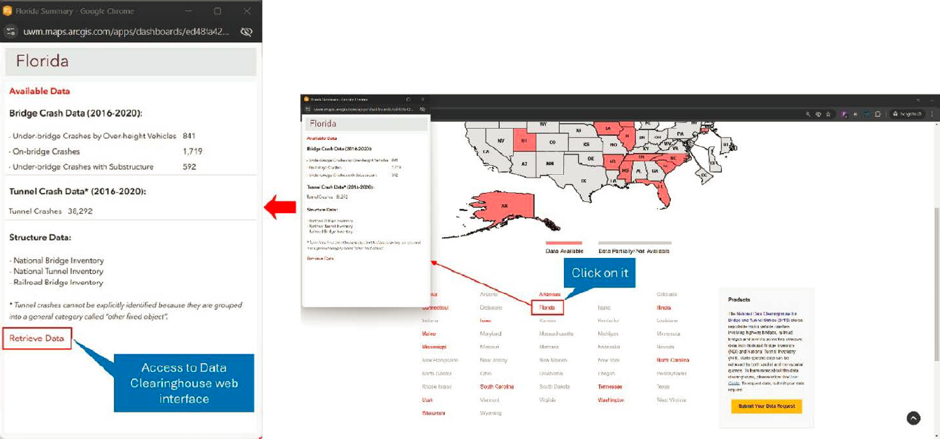
The map on the welcome page displays two color codes: red indicates the data are readily available for direct retrieval using the application; gray indicates the data are partially available or unavailable for the state. To access the Clearinghouse, users can select a state from the map or the list of state names located below the map. After selecting a state, a pop-up dashboard will appear, displaying a summary of data for the state. A link to “Retrieve Data” directs users to the Clearinghouse web interface. Figure 12 demonstrates this operation.
Stagewise Data Clearinghouse Web Interface.
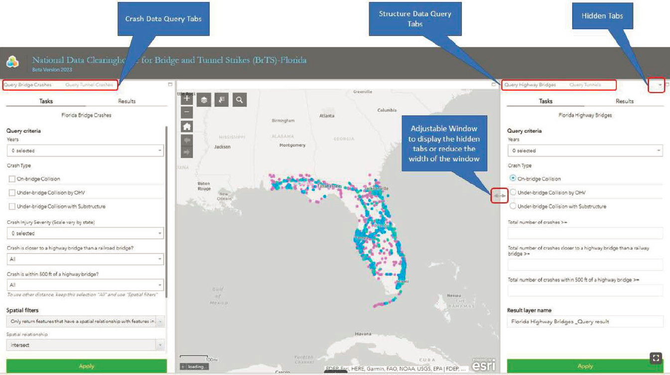
After selecting “Retrieve Data,” the Clearinghouse web interface will appear within a small window that can be enlarged to full screen. The home button is in the upper left corner to navigate to the state. The default view of the web interface displays an empty U.S. map. Users can turn on layers from the “Layer List” in the tool menu on the map to gain a quick visual overview of the data. The key features of the application can be accessed through the Basic Features, Crash Data Query, and Structure Data Query tabs.
Basic Features include the following three functions (illustrated in Figure 13):
- Layer List Feature: provides the layers available for the selected state. It contains crash data and structure data. Refer to the ArcGIS Pro online documentation for more information.
- Search Feature: provides the ability to use an address to locate places on the map.
- Selection Feature: allows users to choose a layer and generate a new layer from the selection. This new layer can be utilized as a relational layer in the spatial filters.
Crash Data Query-related tabs can be found on the left side of the web interface. The tabs include “Query Bridge Crashes” and “Query Tunnel Crashes.” Each tab has two subtabs, “Tasks” and “Results.” The Tasks tab encompasses all the query-related logic, while the Results tab displays the outcome. If a query is left in its default state for a specific field, the query outcome includes all data items in that field.
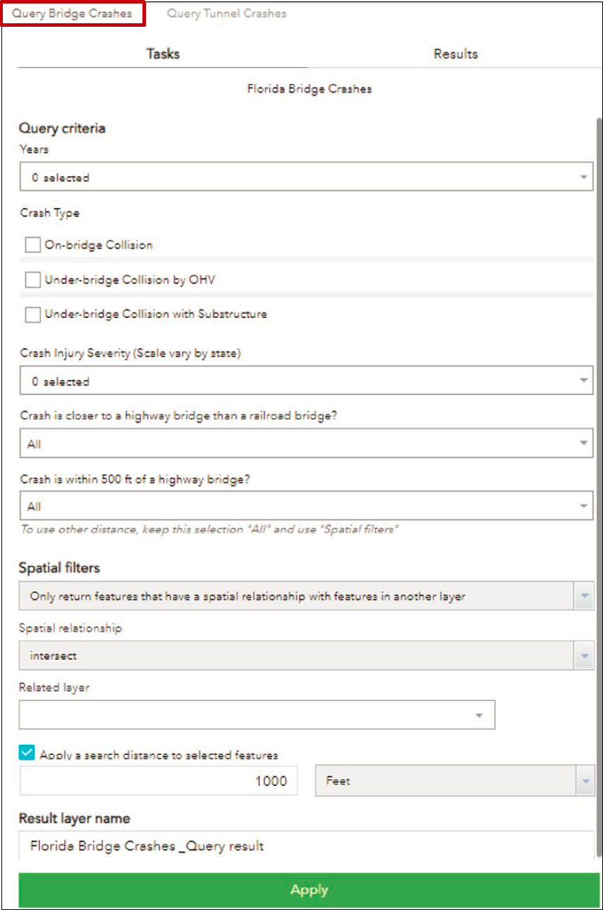
Query Bridge Crashes includes the following five criteria (shown in Figure 14):
- Years: To query crashes for multiple years, use the drop-down menu to select the desired years.
- Crash Type: To retrieve crashes by type, select one or more from the available options.
- Crash Injury Severity (scale vary by state): To retrieve crash data by injury severity, select one or more based on the available options. It is important to note that the values for injury severity may vary by state, with some using letters (A, B, C, etc.) and others using numbers (1, 2, 3, etc.).
- Crash is closer to a highway bridge than a railroad bridge?: The available value options are “All,” “No,” and “Yes.” In a data table, the field name used for this value is “DSCSRL.” A value of 1 is Yes, 0 is No, and a null or blank value is “Not Applicable.”
- Crash is within 500 ft of a highway bridge?: The available value options are “All,” “No,” and “Yes.” In a data table, the field name used for this value is “DSLES500.” A value of 1 in this field is Yes, 0 is No, and a null or blank value is “Not Applicable.”
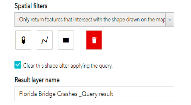
An alternative to querying bridge crashes is to apply spatial filters. For this operation, users have two options for types of spatial filters (shown in Figure 15 and Figure 16):
- Only return features that have a spatial relationship with features in another layer: The query results are determined based on the spatial relationship between the features in the query layer and those in the related layer. Additionally, a search distance can be applied to the geometry of the features in the related layer if desired. It is also possible to utilize the result layer of a previous query.
- Only return features that intersect with the shape drawn on the map: A set of drawing tools is available that allows users to draw shapes on the map to define a specific area of interest.

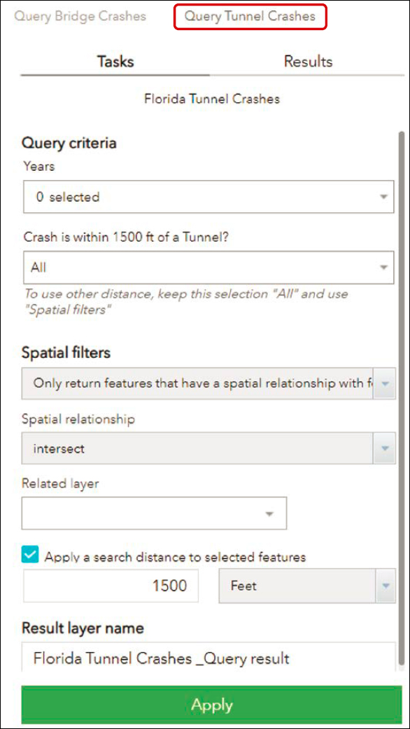
Query Tunnel Crashes includes the following two criteria (shown in Figure 17):
- Years: To query crashes for multiple years, use the drop-down menu to select the desired years.
- Crash is within 1,500 ft of a Tunnel?: The available value options are “All,” “No,” and “Yes.” In a data table, the field name used for this value is “CRS1500FT.” A value of 1 in this field is Yes, 0 is No, and a null or blank value is “Not Applicable.”
The same spatial filters described above for bridge crash queries can also be used for querying the tunnel crashes.
Structure Data Query-related tabs can be found on the right side of the web interface. The tabs are “Query Highway Bridge,” “Query Tunnels,” and “Query Railway Bridges.” Each of these tabs contains two subtabs: “Tasks” and “Results.” The Tasks tab includes all the query-related
logic, while the Results tab displays the query result. If a query is left unchanged for a particular field, the query result includes all records for that field.
Query Highway Bridges includes the following six criteria (shown in Figure 18):
- Years: To query crashes for multiple years, use the drop-down menu to select the desired years.
- Crash Type: To query crashes by type, select one or more from the available options.
- Total number of crashes ≥: Display the highway bridges that have a crash count equal to or greater than the integer value entered. In a data table, the field name used for this value is “SUM_DSALL.”
- Total number of crashes closer to a highway bridge than a railway bridge ≥: Display the highway bridges that have a crash count equal to or greater than the integer value entered and where crashes are closer to a highway bridge than any nearby railway bridge. In a data table, the field name used for this value is “SUM_DSCSRL.”
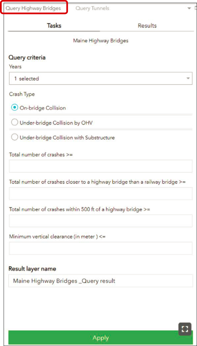
- Total number of crashes within 500 ft of a highway bridge ≥: Display the highway bridges that have a crash count equal to or greater than the integer value entered within a 500 ft radius of the bridge. In a data table, the field name used for this value is “SUM_DSLES500.”
- Minimum vertical clearance (in meter) ≤: Display the highway bridges with a minimum vertical clearance equal to or less than the integer value entered. In a data table, the field name used for this value is “MIN_VERT_CLR_010.”
Additionally, after applying the user-specific query, the results will be displayed and symbolized with the associated “risk score” as shown in Figure 19. As described in the earlier Section 2.3, “Applying Risk Factors to Prioritize Locations,” agencies can assess BrTS risk through various

methods. The risk score is a numeric value indicating the relative risk for each bridge or tunnel based on location-specific characteristics. The risk score supports a proactive approach to identifying and mitigating high-risk locations. Currently, the risk score is only available for the state of Maine. For all other states, the risk score fields contain placeholder values. In this case, the risk score is calculated and normalized for each bridge on a scale of 0 to 100 using the following process:
- Predicted crashes by severity = (predicted crashes) * (predicted % of KABCO injury severities).
- Cost = ∑(comprehensive crash cost by severity * predicted crashes by severity).
- Standardized risk score = 100 * (Total cost – Total costmin)/(Total costmax – Total costmin).
- For display purposes, the Jenks Natural Breaks classification method is applied. The Jenks Natural Breaks method, also known as Jenks Optimization or the goodness of variance fit (GVF), is a data-classification technique for creating choropleth maps by identifying significant data breaks. It excels with multimodal datasets and those with a high variance, for which in our case, the results do show high variance.
The average crash-cost values are based on the recommended national KABCO comprehensive crash unit costs in the FHWA guide, Crash Costs for Highway Safety Analysis (Harmon, Bahar, and Gross 2018).
Query Tunnels includes the following two criteria (shown in Figure 20):
- Years: To query crashes for multiple years, use the drop-down menu to select the desired years.
- Total number of crashes within 1,500 ft of a Tunnel ≥: Display the tunnels that have a crash count equal to or greater than the integer value entered within a 1,500 ft radius of the tunnel. In a data table, the field name used for this value is “SUM_CRS1500FT.”
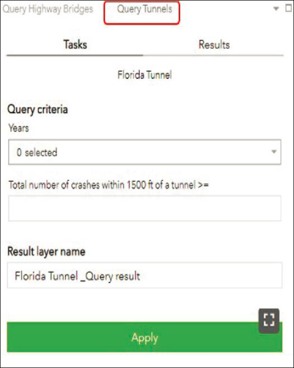
Query Railway Bridges includes the following five criteria (shown in Figure 21):
- Years: To query crashes for multiple years, use the drop-down menu to select the desired years.
- Crash Type: Select one or more from the available options.
- Total number of crashes ≥: Display the railway bridges that have a crash count equal to or greater than the integer value entered. In a data table, the field name used for this value is “SUM_RLDSALL.”
- Total number of crashes within 500 ft of a railway bridge ≥: Display the railway bridges that have a crash count equal to or greater than the integer value entered within a 500 ft radius of the bridge. In a data table, the field name used for this value is “SUM_RLDSLES500.”
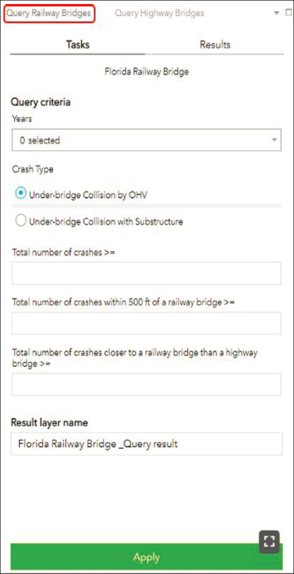
- Total number of crashes closer to a railway bridge than a highway bridge ≥: Display the railway bridges that have a crash count equal to or greater than the integer value entered and where crashes are closer to a railway bridge than any nearby highway bridge. In a data table, the field name used for this value is “SUM_RLDSCSRB.”
All of the abovementioned functions allow users to find specific data based on their interests. After applying the queries, use the following steps to access the options for the query results: generate the results by selecting the “Apply” button, then select the “Results” tab. A drop-down window will appear listing various available options. The operation for downloading the data is illustrated in Figure 22. As shown in the figure, one of the options is to download the results in one of three formats.