Caring for the Individual Patient: Understanding Heterogeneous Treatment Effects (2019)
Chapter: 4 New Methods for the Prediction of Treatment Benefit and Model Evaluation
4
NEW METHODS FOR THE PREDICTION OF TREATMENT BENEFIT AND MODEL EVALUATION
If researchers, patients, clinicians, and payers are to deal effectively with heterogeneous treatment effects (HTE), it will be necessary to develop new methods and models for predicting the benefits and the risks for individuals that are posed by various treatment options. This session looked at various approaches that are available to—or that can be developed by—medical researchers for studying and predicting HTE, focusing on risk modeling based on both genetic data and statistical tools. Much of the information offered in this session was relevant to the patient question: Given my personal characteristics, conditions, and preferences, what should I expect will happen to me?
POLYGENIC RISK SCORES
In the first presentation, A. Cecile J.W. Janssens, Professor of Epidemiology at the Emory University Rollins School of Public Health offered a brief history of efforts to use multiple genes to predict the risk of individuals developing common diseases such as breast cancer and heart disease. The idea is not new, she began. It can be traced back at least 20 years. Little progress, however, has been made in the area since that time.
In the late 1990s, medical researchers began to talk seriously about using genetic information to predict susceptibility to common diseases. In 2002, a paper (Pharoah et al., 2002) published in Nature Genetics titled “Polygenic Susceptibility to Breast Cancer and Implications for Prevention” was one of the first to discuss polygenic susceptibility, she said, and it had one of the first mentions of risk distributions. Specifically, that paper described (1) how certain women had risk distributions for breast cancer that were different from the risk distribution for the general population, and (2) how polygenic risk could be applied in health care to make mammography screening more cost-effective, by identifying those women at greater risk who should be given more frequent screenings. This concept, she explained, is the basic idea underlying polygenic research—that is, using polygenic risk scores to identify high-risk groups for targeted intervention and, more generally, to apply different interventions for different risk groups.
The following year, in 2003, a paper (Yang et al., 2003) appeared in The American Journal of Human Genetics that was the first to describe how multiple genes can be combined to predict risk by using regression analysis. The study focused on posterior risk for carriers of one or more multiple risk alleles, and the particular alleles it examined had strong per-allele effects by today’s standards, with risk ratios between 1.5 and 3.5. The researchers concluded, Janssens said, that it is a promising endeavor to combine multiple variants into a risk score.
In response to that 2003 paper, Janssens and several colleagues, including Ewout Steyerberg, the panel’s moderator, wrote a letter to the editor of the journal arguing that if one wanted to evaluate a polygenic risk score—though it was not called that at the time—it was necessary to include not only high-risk people, but all people, including those who were not carriers of the risk alleles (Janssens et al., 2004). Because the paper’s authors had not done that, the letter contended, the usefulness of the score was difficult to evaluate.
In that same letter, Janssens and her colleagues recommended using a well-established measure called the area under the receiver operating curve, or AUC, to evaluate how predictive a risk score is. In essence, she explained, AUC is an indication of the separation between the risk distributions of those who develop
a disease and those who do not. A small AUC indicates a large overlap among the risk distributions, meaning that the risk score does little to differentiate those who develop a disease from those who do not, while a large AUC indicates that the risk distributions are noticeably distinct. In particular, Janssens said, an AUC indicates how well a measure will be at identifying people who will develop a disease at the cost of how many false positives that might result. “When you want to select the highest-risk group and your AUC is higher, there are more people who will develop the disease in your selected high-risk group, whereas when your AUC is very low, there are many people who will not develop the disease in your high-risk selection. It’s just not as good as you think it is.”
Then Janssens used AUC to discuss the discriminative ability of some polygenic risk scores that were developed a decade ago, before the use of genome-wide association studies (GWASs) became common. For example, a series of studies of type 2 diabetes scores ended up with AUCs that were between 0.55 and 0.60—too small to have much of a separation among the risk distributions. On the other hand, studies of age-related macular degeneration (AMD) and hypertriglyceridemia scores produced AUCs of 0.80—large enough for a substantial significant separation among the distributions.
Generally speaking, she said, the polygenic risk scores with large AUCs rely on common variants with strong effects on a person’s risk. She compared, for example, the gene variants that went into the two risk scores, one for type 2 diabetes and one for hypertriglyceridemia. The type 2 diabetes risk score, which produced an AUC of 0.60, relied on 18 gene variants, none of them with a risk ratio larger than 1.36 and half of them 1.10 or less. By contrast, the hypertriglyceridemia risk score used only seven variants, but they all had risk ratios between 2.10 and 7.36 (Lango et al., 2008;Wang et al., 2008).
One possible way to use genetic factors to predict risk would be to combine them with traditional risk factors and see if the additional genetic information increases the predictiveness. In 2008, she and a colleague reviewed a dozen papers that took that approach (Janssens and van Duijin, 2008), and they found that the addition of information about genetic variants to the traditional risk factors increased the AUC by 0.06 or less and, in most of those studies, by 0.02 or less. In other words, the added genetic information did very little to improve the ability to distinguish those who would develop a disease from those who would not. The genetic information, while interesting, did not have clear clinical implications in terms of modifying how a doctor would approach a particular patient.
Summing up the experiences from that time period, Janssens commented that researchers were still learning how to use the relevant methods, and relatively few genes had been identified, so perhaps no great impact should have been expected.
Other shortcomings included that researchers paid little attention to what the clinical uses of their work might be, they used non-representative populations, they provided no relevant comparisons with clinical risk models, and they tended to rely on p-values instead of AUC—they were just not paying attention to actual improvements in predictions. To be fair, she said, the researchers themselves reported that the methods had limited predictive power, but people believed that once the whole human genome became accessible, the predictive power should improve. “The door was wide open for GWAS to deliver,” she said. “The future was still bright.”
Indeed, in the past year, she has seen an increased interest in polygenic risk scores. She offered a sampling of headlines predicting that genetic scores would make it possible to predict such things as heart disease, breast cancer, Alzheimer’s disease, and even intelligence and reading ability. “You ask yourself, What has changed in the meantime?” she said. “Have all these genes that have been discovered delivered so much?” The answer is no, she said. “The risk distributions are still largely overlapping for the same diseases.” She then showed a recent paper using polygenic risk score to predict ovarian cancer. The risk score relied on 96 single-nucleotide polymorphisms (SNPs), and yet the AUC was only 0.60. And a genome-wide risk score that used 6.6 million variants to predict coronary disease had an AUC of only 0.64 (Khera et al., 2018). Using the entire genome to generate a risk score does not do much more—at least in this case—than the studies a decade ago that relied on just a few genes or, indeed, risk scores generated from traditional risk factors.
Why then, she asked, are the people performing these studies claiming to be predicting something? The answer, she said, is that what geneticists mean by prediction is very different from what clinicians expect from prediction. She quoted a recent article by Carl Zimmer that appeared in The Atlantic:
When geneticists use the word prediction, they give it a different meaning than the rest of us do. We usually think of predictions as accurate forecasts for particular situations.… Geneticists are a lot more forgiving about predictions. (Zimmer, 2018)
When geneticists speak of “prediction,” Janssens further explained, they are generally referring to weak effects with little or no practical or clinical significance because the scores do little to differentiate among groups of people.
Concluding, Janssens noted that the shortcomings of polygenic risk studies today are the same as they were a decade ago. Generally, no consideration is given to the intended use, so there is no way to tell whether the predictive performance
is sufficient. The risk thresholds, if they are chosen at all, are based on little to nothing. There is no calibration, no validation, and no appropriate comparison with clinical models. “I think you can hear the frustration in my voice,” she said. “A lot of people are calculating these polygenic risk scores, but they have no clue what can be done with them.” Of course, there are exceptions, but this is her overall impression of the field. The problem is that genetic researchers are generating a lot of research results without any framework to understand whether the results will ever be relevant.
In closing, she quoted an article published in The New England Journal of Medicine:
In our rush to fit medicine with the genetic mantle, we are losing sight of other possibilities for improving the public health. Differences in social structure, lifestyle, and environment account for much larger proportions of disease than genetic differences. Although we do not contend that the genetic mantle is as imperceptible as the emperor’s new clothes were, it is not made of the silks and ermines that some claim it to be. Those who make medical and science policies in the next decade would do well to see beyond the hype. (Holtzman and Marteau, 2000)
“We are long past that ‘next decade,’” she stated, “but I think that it still applies today.”
Frank Harrell, Professor of Biostatistics at Vanderbilt University offered several comments on Janssens’s presentation. He began by referring to it as appropriately pessimistic, commenting that genetics had not had—with some exceptions—a good track record in being predictive of outcomes. Referring to a paper published by other researchers at Emory (McGrath et al., 2013) and whose results were featured in The New York Times (Friedman, 2015), Harrell said, “We get involved in sexy things, and we forget to do the simple things.” The findings in the paper that were picked up by the press related to using brain imaging to determine whether a patient would respond better to psychotherapy or drug therapy with antidepressants. Harrell said it was unlikely that part of the study would be replicated, but hiding in one of the paper’s tables was a result that, while unsexy, had useful clinical implications: Patients with high anxiety levels responded very differently to psychotherapy than to drug therapy. Precision medicine faces a similar issue, he postulated, predicting that if people in the field are not careful they will end up excelling in “precision capitalism,” that is, receiving plenty of grants, but not so much in improving public health. He referred to Janssens’s presentation as a “wakeup call” to that possibility.
PROMISE OF MACHINE LEARNING
With the availability of high-speed, high-powered computers, it has become possible not only to quickly analyze large amounts of data, but also to analyze such data in ways that were not feasible before. One such method is machine learning, through which computers search for patterns in data rather than analyzing the data in a predetermined way. Machine learning makes it possible to spot correlations in data that may have never been considered by the machine’s human operators and that may not even seem to make sense at first.
In the session’s second presentation, Fan Li, Associate Professor of Statistical Science at Duke University described machine learning and discussed how it might be put to work analyzing HTE. Right now, “HTE and machine learning are two buzzwords in comparative effectiveness research,” Li said. The use of machine learning to explore HTE has become a hot topic, especially in cases when there are large amounts of data. “The central goal from a statistical standpoint,” she said, “is the same as the traditional regression methods: to accurately learn from the data what the outcome function is, given the covariates and the treatment variable. The goal is the same; it’s just some new analytical methods.” These machine learning methods are generally more flexible and adaptive than the traditional methods, she added, but they are not a panacea. They have their own limitations.
For the duration of her presentation, Li focused on four specific machine learning approaches that are popular methods for application to HTE:
- Penalized regression (e.g., least absolute shrinkage and selection operator [LASSO], elastic net regularization);
- Regression tree-based methods (e.g., classification and regression trees [CART], random forests);
- Bayesian nonparametric models (e.g., Gaussian processes, Bayesian trees); and
- Ensemble learners (e.g., boosting, forests).
“These are all supervised learning methods,” and in their original form they are used for prediction, not estimation, she said. In statistics, there is a subtle difference between prediction and estimation—in that, prediction uses observed data on one set of variables to guess at the value of a different variable, and estimation uses observed data to guess at the true value of an underlying parameter. Applying these supervised learning methods to HTE requires that they be modified somewhat. The basic problem, she explained, is that you want to see how a given individual will do under a certain treatment condition versus how that same person would
do under a different treatment condition. “You never see that at the individual level,” she said. “That is the fundamental problem of HTE.” Over the past 25 years, however, there has been a great deal of work to adapt machine learning models to this sort of analysis, and there are now a variety of machine learning techniques that can be used to predict HTE.
The first of her machine learning approaches—penalized regression—has been used a great deal in work with HTE, Li said. “You do not penalize regression,” she explained. “You penalize the complexity of regression.” A HTE regression analysis is essentially examining the interactions between the treatment variable and multiple covariates. But many of those interactions are not particularly important in understanding the treatment effects, and you can throw those out without losing much analytical power. “This type of regression essentially has a way to select the most important and meaningful interactions,” Li said—and thus avoid overfitting.
Next, she explained regression trees. They get their name because the covariate space is partitioned into subgroups that are referred to as “leaves.” The analysis proceeds by predicting responses in each leaf using the sample mean in that region. At each step, researchers review the variables and decide whether and where to split the sample into different leaves, with the tree’s complexity growing as more leaves are put in place. Cross-validation is used to make decisions about the tree’s complexity—in essence, how deep the tree’s branching will be—and about how parts of the tree can be “pruned” to reduce its complexity. The technique was originally developed for prediction, Li said, but in 2016, it was modified for use with HTE in what Li referred to as a “landmark paper” (Athey and Imbens, 2016). It is just one of what Li said are “probably hundreds of papers written in the past few years about doing this sort of analysis.”
There are several advantages to the regression tree approach. There is a large selection of available software that can be used to implement it, for instance. It is fast, and it is easy to interpret. Additionally, while a single tree may be a “weak learner,” one can average over a collection of trees—called a forest—to improve the estimates. The disadvantages of the regression tree approach, she said, are that the trees tend to underestimate uncertainties, and that the structure of the trees lacks the flexibility of some of the other methods.
The third approach is Bayesian nonparametric models. Li described two types of Bayesian approaches: Bayesian trees (which are similar to a regression tree except that they are implemented under the Bayesian paradigm, using prior knowledge) and Gaussian process models. Generally speaking, Bayes’ theorem is an approach to calculating probabilities that begins with a certain amount of prior knowledge—unlike traditional statistics, for which the calculations depend
completely on the data that are collected—and then modifies the probabilities as more and more data come in.
Discussing the pros and cons of Bayesian nonparametric methods, Li said that the pros include the fact that you can incorporate prior knowledge into the model, the model quantifies uncertainties automatically, it works well with small samples, and it is “elegant,” which makes it appealing to mathematicians. One of its biggest cons is that these approaches are difficult to scale—as the amount of data grows, the required computational resources increase rapidly. Furthermore, these approaches can be difficult to explain to a lay audience, software for implementation is limited, and having to choose and justify prior distributions before getting started is an additional complication.
The fourth type of approach Li described is ensemble learners. In any of the first three approaches, she said, a single model can be a weak learner. “The performance might not be good. So, the idea is to make a bunch of models and combine them. That’s where the name ‘ensemble learning’ comes from.” A forest is one type of ensemble—in this case, when you assemble a bunch of trees—but the same idea can be applied to other models, as well.
Summarizing her presentation, Li highlighted several points. First, there has been a great deal of work recently on machine learning theory, both in statistics and in economics, but there is still much to learn about applying it to health statistics and HTE. There are still relatively few applications that have been developed, and “there’s a huge gap between theory and practice here.” Thus, more translational work is needed. In the past couple years, researchers have developed several new methods for use with HTE that are being offered to those in the health field. However, Li said, there is little that is known about the “empirical, comparative performance of those models,” and that issue needs to be addressed. Software development will also be key to using machine learning to analyze HTE. Many of the methods she described have available software that no one is using because people in the HTE field are not yet familiar with it. A change will require effective collaboration between the methodologists—the statisticians, the machine learning researchers—and the clinical researchers, Li said. Finally, she said, “One must organically fuse traditional statistical tools and machine learning to reach better comparative effectiveness research.” It will not work simply to “put one upon the other” because there are a number of subtleties about combining the traditional statistical tools with machine learning that must be worked out.
Frank Harrell also commented on Li’s presentation. One of her key messages, he said, was that machine learning methods are very flexible, but they are also “data hungry.” Referring to a paper by Ewout Steyerberg and colleagues, he noted that machine learning analyses could require as much as 10 times the sample size that
traditional regression analyses require (Steyerberg et al., 2014). Regarding the various models that Li described, Harrell said, “To me, the method that has the most promise of anything in this space is ordinary Bayesian parametric models” because of the possibility of using expert opinion to guide both the studies and the data collection.
METHODOLOGICAL ISSUES RELATED TO PREDICTIVE SCORES
Patrick Heagerty, Chair of Biostatistics at the University of Washington School of Public Health, discussed some technical issues related to developing and evaluating predictive scores. “What can we say from the data that we collect and the analyses that we produce?” he asked. “I want to emphasize limitations in our ability to make specific statements.”
Generally speaking, Heagerty said, there are three levels at which one can analyze risk. The first is the individual patient level, for which one ideally would like to make predictions. Generally, however, such predictions are not feasible because it is impossible to observe outcomes under counterfactual treatment conditions in an individual. Consequently, what happens is that one makes predictions at the level of a stratum—a group of individuals with similar characteristics. This is the second level. The third is the population level, which is the level that is most important when talking about maximizing performance. He then spoke briefly about the recent work in prediction in the field of statistics, emphasizing at which level (i.e., individual, stratum, population) the work was being carried out. He also noted the work of Susan Murphy, who focused on identifying rules for treatment programs at the individual level followed by measuring the effects of those rules at the population level (Qian and Murphy, 2011).
One quantity of interest is referred to by statisticians simply as “the value,” he said; yet, it is actually the mean population outcome under the targeted treatment. Two approaches are used to determine the population mean. One is Q-learning, in which one estimates the mean under both treatment and control and compares them; one can then recommend treatment based on whichever mean is better—a rule that will ultimately lead to a better population mean, he said. The other is outcome-weighted learning, in which one skips the outcome model and directly makes a prediction rule that optimizes performance at the population level. In both approaches, the focus is on decisions at the individual level but performance at the population level. “That’s the first message that I really want to emphasize.” He continued, “Many contemporary methods consider action at the individual level but still measure performance at the population level. I think it is appropriate, but there is a disconnect.”
Haggerty next arrived at his second main point: Most attempts to define “patients who benefit” are unreliable because they rest on outcome-based definitions that are fundamentally not measurable, owing to the fundamental problem of causal inference for individuals. Because researchers cannot observe the outcome under an alternative treatment for a given patient, “it’s very difficult to migrate some of the tools we’ve used traditionally for diagnostic and prognostic methods. We heard this said at least twice today, and I’ll just make it a little more formal.” The ultimate goal, he noted, is to find predictive markers, or markers that can be used to guide treatment for individuals. But what, he asked, does it even mean to talk about individual benefit? “What do we mean when we say ‘patients who benefit from treatment’? Can you label those patients for me, the patient [who] will benefit from treatment? And the fundamental answer is no.” Why? Determining which individuals will benefit from treatment requires that we know how that patient would fare if treated and if not treated—which is impossible since a patient cannot be both treated and not treated.
To formalize this notion, Heagerty presented a figure listing the various possible outcomes for a patient undergoing treatment (see Figure 4-1). In this simplified world, outcomes are either positive or negative, with no gradations. There are four possibilities for how an individual patient will respond: positively if left untreated and positively if treated (i.e., neutral between treatment and no treatment); positively if left untreated and negatively if treated (i.e., worse outcome with treatment); negatively if untreated and positively if treated (i.e., benefit from treatment); and negatively if untreated and negatively if treated (i.e., neutral). Ideally, a clinician would like to know in which row of the figure a given patient fits to inform treatment decisions. The fundamental problem, however, is straightforward, Heagerty said. “We can see data for untreated people, whether they get better or not or whether they do well or not. We can see it for treated people, as well.” But, as he previously mentioned, you do not know how each untreated individual would have done with treatment or how each would have done without treatment.
These four categories can also be viewed as “principal strata.” In this regard, Heagerty mentioned the principle stratification framework, introduced by Constantine Frangakis and Donald Rubin (2002), as one approach to estimating the causal effects of treatment. Heagerty alluded to the controversies over the appropriate uses of this causal inference framework, citing contradictory papers (i.e., Janes et al., 2015; Simon, 2015), which were published in the same issue of Journal of the National Cancer Institute.
Notably, it is possible to sidestep the limitation of unobservable counterfactual outcomes, he said—particularly when the outcome of the treated or the untreated
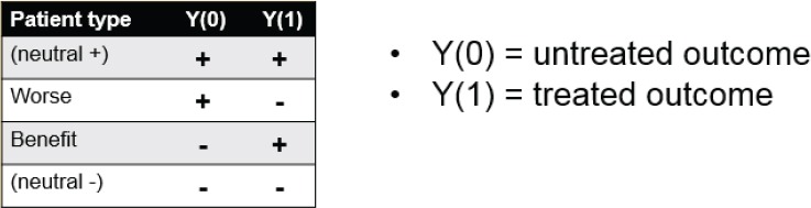
SOURCE: Patrick Heagerty presentation on May 31, 2018.
condition is relatively uniform. Suppose, for example, that you limit yourselves to a group of patients who will clearly have a negative outcome without treatment. “This may be some oncology setting where we think that without treatment people will do poorly,” he said. In this case it is only necessary to know how a patient will do with treatment. The critical question then becomes, Is there a biomarker or some other measure that separates people who will do well under treatment from those who will do poorly? “In this one setting we can start to migrate tools for classification or prediction,” he said. A second situation in which the problem can be sidestepped is when the treatment is expected to always—or almost always—have a positive outcome. In this scenario, the prediction issue is simplified to an issue of prognosis: Who is at greatest risk if left untreated, and who will likely be fine without treatment? In that case, there are several tools that can be brought to bear (Steyerberg et al., 2010).
Furthermore, there are situations in which one can measure both conditions—to see how a patient will fare with and without treatment. Describing the “N-of-1” trial approach, Heagerty suggested that patients with pain, for instance, can be treated first with a pain medication for a period of time and then with a placebo, or vice versa, and the outcomes compared. This is not a perfect solution, however, as other variables may change over the time periods of treatment. “There are still identifiability problems in this space,” Heagerty explained. “It also invites other questions, like, Is that really the goal, whether my one outcome is better than my other one outcome? Or is it really my mean outcome, repeatedly treating me one way and repeatedly treating me another way?” That said, Heagerty reiterated his second main point, “I think attempts to define ‘patients who benefit’ … can lead to an outcome-based definition that just is not measurable. This is a fundamental problem about talking about the performance of classifiers for [whom] should get treated.”
Regarding his third point, Heagerty described the use of scores. In particular, he spoke of the score as the difference between treated risk and untreated risk.
“For given characteristics, what’s the difference if I’m treated as compared with if I’m not treated?” Noting that many people in the workshop discussed the importance of prognosis—knowing what is going to happen in an untreated patient—he emphasized the importance of prediction scores, that is, predicting what will happen to a treated patient. “I think the fundamental goal is to try to learn that predictive score, the benefit that would be assigned to a given patient,” he said. “I want to push us to say, ‘Yes, it’s important to look at baseline, untreated, prognostic risk, but let’s at least start to try to get scores that measure the ensemble, aggregate expected benefit,’” rather than just prognostic risk.
The impetus for scores comes from the fact that it is impossible to validate statements about an individual, he said. “It’s too small of a group.” What can be done, however, is to make statements about people with a given quantitative score and then validate that score. “That’s my third main point,” he said. “Methods should consider development of action at the individual level, but that action is based on a score, and the score can be validated locally. We can validate whether that score is giving an accurate representation of the expected benefit of being treated as compared with not treated.”
In response to a question from the audience, Heagerty acknowledged the importance of knowing and communicating about the methods and data used to generate predictive models for a particular patient. “I feel like we don’t do a good job of showing the source data that generated that prediction,” he said, “and we could and should.” Importantly, researchers should clearly indicate whether the data used to create a model truly applies to the patient. As an example, he referred to an 82-year-old patient discovering that a study used to create a prediction model involved only patients much younger than 82 years—which would be important information. “We have a responsibility to communicate better the evidence base that generates those predictions,” he said.
ABSOLUTE RISK VERSUS RELATIVE RISK
In his response to the presentations, Michael Pencina, Vice Dean for Data Science and Information Technology at the Duke Clinical Research Institute raised an issue that would be touched on at various points throughout the workshop: absolute versus relative risk. Absolute risk refers to the chances of something happening over a particular period of time—for example, the chance of a person having a stroke over the coming year. Relative risk refers to the difference in risks between two situations—for example, the risk of having a stroke over the coming year if you take a particular drug versus if you do not. “The absolute risk reduction is a key metric,” Pencina said. “It’s composed of two
pieces. It’s the risk, and it’s the relative risk reduction. These two pieces are critical, and you can’t focus just on one.”
Building on this point, David Kent later commented that “HTE is a scale-dependent concept—you just have to specify the scale. And the issue is that for clinical decision making the most important scale is the absolute scale.” The idea that HTE only exists when there is significant variation on the relative scale has served the field poorly, he said. “I think we’re a little brainwashed by that distinction. We should always look at the absolute risk scale.” Instead of focusing on a search for “statistically significant” relative effect modifiers one variable at a time, the approach needs to provide the kind of evidence that will be helpful to doctors and patients as they are making decisions—one patient at a time.
This page intentionally left blank.


