Future Directions for Southern Ocean and Antarctic Nearshore and Coastal Research (2024)
Chapter: 3 The Impact of Antarctica and the Southern Ocean on Global Sea Level
3
The Impact of Antarctica and the Southern Ocean on Global Sea Level
The Antarctic ice sheets are the largest bodies of frozen water on Earth. The West Antarctic Ice Sheet (WAIS) and East Antarctic Ice Sheet (EAIS) together store about 27 million km3 of ice, with a potential global eustatic sea level1 equivalent of 58 m (Fretwell et al., 2013; Hanna et al., 2020). Sea level rise projections, based on relatively well-understood ice mass balance processes, indicate a likely sea level rise of approximately 0.6 m relative to a 2020 baseline by the year 2100 (see Figure 3-1; Fox-Kemper et al., 2021). In contrast, assessments that include hypothetical and poorly understood grounding zone instabilities that may occur in Antarctica project from around 1.6 to 2.3 m of sea level rise by 2100, with further accelerated rise beyond 2100 (Fox-Kemper et al., 2021). Given the limited understanding of ocean–ice interaction, especially related to grounding zones of Antarctic ice sheets, these higher estimates may still be too low (Siegert et al., 2020). Improved projections of sea level rise in the near and long terms are essential to protect the global community and economy, especially the 11 percent of the global population (roughly 1 billion people) that lives in low-lying coastal zones (Neumann et al., 2015a). In addition to the potential loss of life, these imperiled areas also generate about 14 percent of the global gross domestic product (Magnan et al., 2022). Given that the cost of adaptation to sea level change along U.S. coastlines is expected to exceed $1 trillion by 2100 (Neumann et al., 2015b), accurate projections of sea level rise will enable timely investments that can target areas at greatest risk. Thus, there is an urgent need to understand the processes driving contemporary ice mass loss and the long-term trajectory of sea level rise in order to protect the welfare of global and U.S. coastal communities and economies.
From 1901 to 1971, global mean sea level (GMSL) rise averaged about 1 mm/year and was dominated by net melting of glaciers and regional ice caps. Thermosteric effects2 from global ocean warming became important around the 1970s, and sea level rise further accelerated to more than 3.5 mm/year between 2006 and 2018, as melting in Greenland matched the integrated melting of isolated glaciers and ice caps. Net loss of grounded ice from Antarctica is, so far, a minor contributor to sea level rise (less than 10 percent of the current rates). However, a variety of sustained orbital remote sensing datasets show that the Antarctic ice sheets have been losing net mass to the ocean at an accelerating rate, from about 49 gigatons per year (Gt/y) in the 1990s to roughly 215 Gt/y over the last decade (e.g., IMBIE Team, 2018; Rignot et al., 2019; Smith et al., 2020). The Intergovernmental Panel on Climate Change’s (IPCC’s) Sixth Assessment Report projects that sea level rise will begin to be dominated by ice losses in Antarctica sometime between the mid-21st and 22nd centuries, depending on emission scenarios (Figure 3-2).
___________________
1Eustatic sea level is the global average sea level.
2Thermosteric effects are changes in heat content that affect sea levels.

NOTES: SSPs link fossil fuel emissions to socioeconomic developments (e.g., sustainable development, regional rivalry, inequality, fossil-fueled development) to facilitate the integrated evaluation of climate impacts, vulnerabilities, adaptation, and mitigation. Solid and dash-dotted grey lines are extrapolations of the 1993–2018 satellite altimeter trend. Dashed and dotted pink lines are low confidence, but plausible worst-case scenarios for poorly constrained processes integrating a single model implementation of marine ice cliff instability and other potential instability mechanisms (DeConto et al., 2021), as well as structured expert judgment of the potential impact of poorly constrained ice sheet processes (Bamber et al., 2019). Projections and likely ranges at 2150 are shown to the right of the graph. Lightly shaded thick and thin ranges show the 17th–83rd and 5th–95th percentile ranges, respectively.
SOURCE: Modified from Fox-Kemper et al., 2021.
Longer-term model projections, beyond the year 2100, are given low confidence by IPCC due to limited knowledge (Fox-Kemper et al., 2021). However, these models hypothesize that ice losses will continue and will be essentially irreversible for the next 10,000 years under all emissions scenarios, even if net greenhouse gas emissions are reduced to zero over the next few centuries (Figure 3-2). Garbe et al. (2020) identified that if ice is lost at global warming levels ranging from 2°C to 10°C, it will not regrow until global temperatures are a degree or more cooler than preindustrial temperatures. Additional models suggest that even stabilizing the climate at 2100 levels will still lead to ice loss from Antarctica and sea level rise lasting until at least the year 3000 (Chambers et al., 2022; Golledge et al., 2015). Thus, humanity has committed to some level of sustained sea level rises lasting centuries or millennia based on carbon emissions that have already occurred (Clark et al., 2018). There is therefore an urgent need to accurately project the rate and location of sea level rise, in order to plan for the welfare of coastal and global communities and economies.
Accurate predictions of sea level rise require a fundamental understanding of the controls on Antarctic grounded ice sheets, as well as the protective and buttressing power3 of the floating ice that extends from them. The stability of ice sheets and ice shelves, and the associated predictions of sea level rise, are strongly affected by ocean, and to a lesser extent, atmospheric forcing (Figure 3-3; Dutrieux et al., 2014a; Paolo et al., 2015; Pritchard et al. 2012). Other factors—including solid Earth isostatic rebound4 (Barletta et al., 2018), geothermal heat flux (Seroussi et al., 2017), and subglacial hydrology (Ashmore and Bingham, 2014)—also affect the rate of mass loss in the Antarctic by controlling the basal conditions of ice sheets and impacting the relative distribution of sea level rise across the globe.
___________________
3Buttressing is the resistive stress that is exerted by floating ice on grounded ice (Paolo et al., 2015).
4Isostatic rebound is the rise of land that was depressed by the weight of ice sheets (NSIDC, 2023).
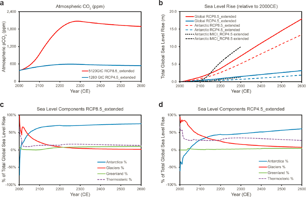
NOTES: Representative concentration pathways (RCPs) describe scenarios that include time series of emissions and concentrations of the full suite of greenhouse gases, aerosols and chemically active gases, as well as land use/land cover (Moss et al., 2008). RCP4.5_extended is a low-emissions scenario without active carbon sequestration, which yields warming of ~1.3°C in 2100 CE and ~2°C in 2600 CE. RCP8.5_extended is a high-emissions scenario with no significant CO2 mitigation, which yields warming of ~4°C in 2100 CE, rising to ~7°C in 2600 CE. (a) pCO2 = partial pressure of CO2. (b) Projected sea level rise (global and the component from Antarctica) based on two models: Clark et al., 2016 (dashed red and blue lines), which excludes marine ice cliff instability (MICI), and DeConto et al., 2021 (black dashed and dotted), which includes MICI; inclusion of MICI causes acceleration of Antarctic ice loss after 2100 CE in the high-emissions scenario and has little effect in the low-emissions scenario. (c) Percentage of sea level rise within MICI feedback due to various components under RCP8.5, projects Antarctic ice losses beginning to dominate global sea level rise in the mid-21st century CE. (d) Percentage of sea level rise due to various components under RCP4.5 (Clark et al., 2016), projects Antarctic ice losses beginning to dominate global sea level rise in the mid-22nd century CE.
SOURCE: Data from Clark et al., 2016; DeConto et al., 2021; Meinshausen et al., 2011.
Controls on marine-based sectors of ice sheets (which are grounded below sea level) are particularly important to sea level–rise predictions as they are sensitive to oceanic forcing (Joughin et al., 2012). This means these sectors of ice sheets are easily influenced by changing ocean properties, especially ocean temperatures and the distribution of warming with depth (Chapter 4). The WAIS is one example of a rapidly changing marine-based ice sheet, as it contains large areas that are grounded below sea level. One of the three major subglacial basins5 in Antarctica, the Byrd Subglacial Basin, is found within the WAIS (Figure 3-4). The Byrd Subglacial Basin’s vulnerability to collapse has been inferred many times (e.g., Mercer, 1978), and it currently contains the fastest-thinning glacier
___________________
5Subglacial basins are topographic depressions in ice sheets that hold large reservoirs of sea level potential, as their beds lie below sea level.
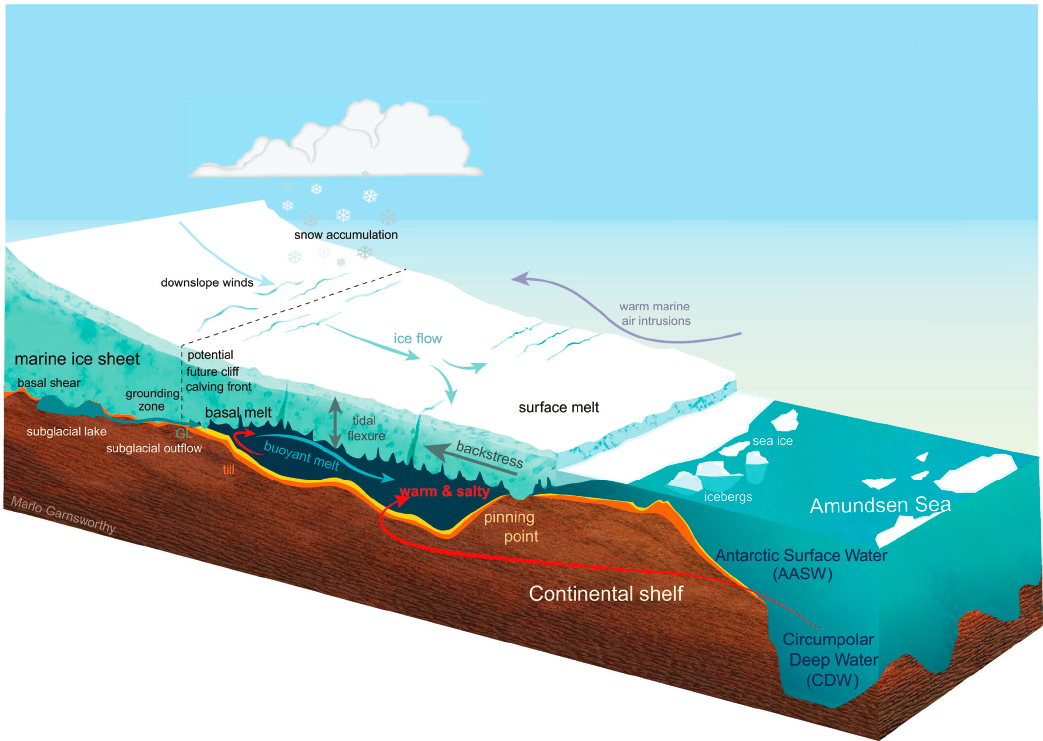
NOTES: Circumpolar Deep Water is warmer and saltier than the surrounding water masses and can reach the grounding zone of marine ice sheets. Other processes like tidal flexure, warm marine air intrusions, snow accumulation, and downslope winds can also affect the mass balance of ice sheets.
SOURCE: Larter, 2022.
in all Antarctica—the Thwaites Glacier. The collapse of the WAIS alone would contribute approximately 3.2 m to global sea level (Bamber et al., 2009). Although the potential for the WAIS to collapse exists, the reality, timing, and rate of collapse remain uncertain. The temperature threshold for collapse is estimated at approximately 1.5°C global average warming—a level that will likely be exceeded by 2027 (WMO, 2023). The timescale of collapse is tentatively estimated at 2,000 years in the future (McKay et al., 2022), but this is uncertain as ocean warming and delivery to ice shelf cavities, rather than global atmospheric temperature, are key controls (Arthern and Williams, 2017). For comparison, Golledge et al. (2021) summarize evidence for a collapsed WAIS in the Amundsen Sea region during the Last Interglacial (LIG; 126,000 years ago), a time of global warming of 0.5°C to 1.0°C relative to preindustrial levels. Based on this past record, Golledge et al. (2021) suggest that current ocean warming is sufficient to trigger collapse of the WAIS, with most rapid collapse and peak rates of sea level rise projected 1,500–2,000 years from now. However, Berends et al. (2023) note that predictions of the timing and rate of ice loss are strongly dependent on parameterization of subshelf melting, which is poorly known. Van Westen and Djkstra (2021) note that low-resolution models that lack the ability to model eddies may overestimate subsurface ocean warming.
The EAIS is the world’s largest ice sheet and contains more sea level potential than the WAIS (the equivalent of about 50 m; Garbe et al., 2020). While the EAIS is traditionally regarded as less sensitive to climatic changes than
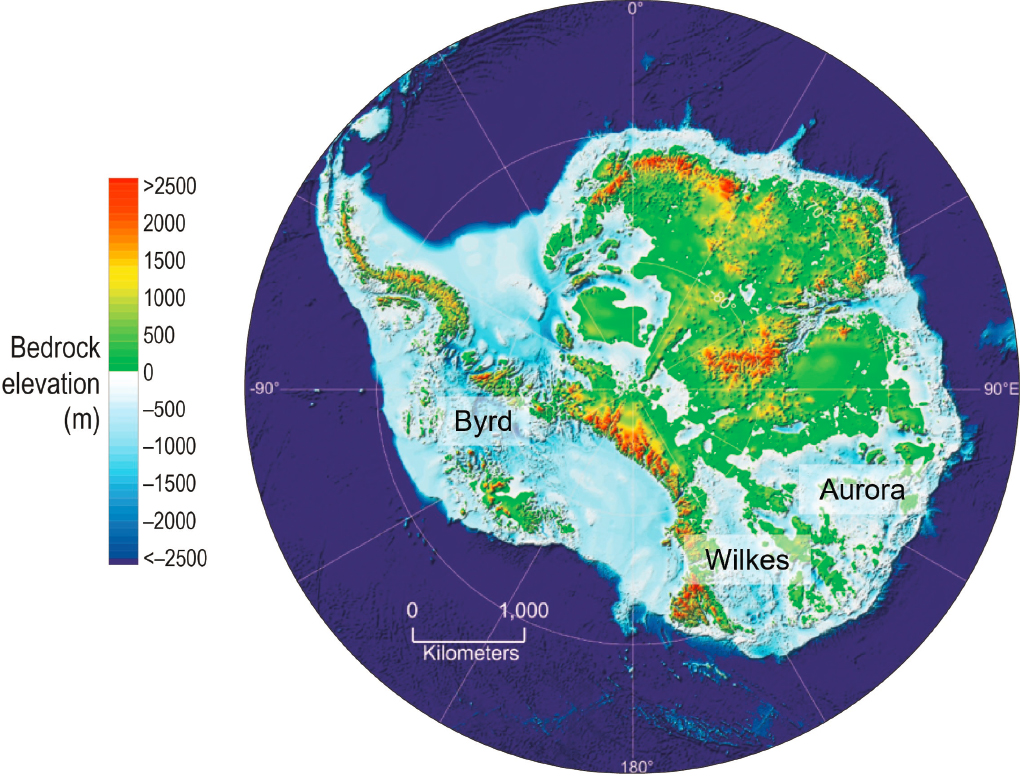
NOTE: Labels indicate the subglacial basins in the West Antarctic Ice Sheet and in the Pacific sector of the East Antarctic Ice Sheet (Byrd, Wilkes, and Aurora).
SOURCE: Revised from Oppenheimer et al., 2019.
the WAIS, the stability of the Pacific sector of East Antarctica may have been overestimated (DeConto and Pollard, 2016; Golledge et al., 2017; Li et al., 2016; Mohajerani et al., 2018; Rignot et al., 2019; Smith et al., 2020). This sector holds two major subglacial basins—the Aurora and Wilkes Subglacial Basins. The Wilkes Subglacial Basin contains 3–4 m (Mengel and Levermann, 2014) and the Aurora Subglacial Basin contains about 5 m (Greenbaum et al., 2015) of sea level potential. The Totten and Denman Glaciers are the primary outlets of the Aurora Subglacial Basin, and an unnamed glacier draining into the Cook Ice Shelf is the primary outlet of the Wilkes Subglacial Basin. Totten and Denman have been the fastest-thinning glaciers in the EAIS for the entire satellite altimetry record (e.g., Smith et al., 2020; Zwally et al., 2015). Although the major outlets of the Wilkes Subglacial Basin have not been thinning rapidly, analyses of proxy data from offshore and subglacial geomorphological studies indicate that both the Wilkes Subglacial Basin and Aurora Subglacial Basin likely collapsed during past warm periods (Cook et al., 2013, 2014; Gulick et al., 2017; Wilson et al., 2018; Young et al., 2011). In particular, the Wilkes Basin, which borders the western Ross Sea, is believed to have undergone a grounding line retreat of about 700 km inland from its current position during a global warm period roughly 400,000 years ago, contributing 3–4 m to the global sea level (Blackburn et al., 2020; Wilson et al., 2018). Recent estimates for these EAIS basins suggest the temperature thresholds that could initiate collapse are near 3°C and that collapse could occur less than 2,000 years in the future (McKay et al., 2022).
Likely ice loss rates are poorly constrained, in part because of limited information about the processes occurring at ice grounding zones (e.g., DeConto et al., 2021), and in part because the warming associated with projected ice loss is unprecedented in human history. The paleoclimate record is the primary source of information for verifying these projections and refining understanding about rates of long-term change. Comparison of model projections of global sea level reconstructions provides plausible hypotheses for the variability of Antarctic ice over the Cenozoic time,6 particularly in the marine-based sectors of the WAIS and EAIS (Escutia et al., 2019; Levy et al., 2022). However, predictions of sea level rise for 10,000 years in the future are less than reconstructed sea level in the LIG, when sea level was 6.6–9.4 m higher than at present (Kopp et al., 2009). This suggests that the predictive models may not be sensitive enough because the global warming that occurred in the LIG (about 126,000 years ago) was only 0.5°C to 1.0°C, which is within the range of current anthropogenic warming (Clark et al., 2020; Golledge et al., 2021). In contrast, GMSL projections for 10,000 years in the future are within the range of reconstructed sea levels for the Mid-Pliocene Warm Period (MPWP), the last time global concentrations of CO2 surpassed 400 ppm, which led to average sea levels between six and several tens of meters above present (Dutton et al., 2015). Nevertheless, the large uncertainty of these projections suggests the need to refine process understanding for models and geologic verification data.
Important sources of geologic verification are provided by the prehistorical extents and rates of ice advance and retreat near the Antarctic continent derived from ice-proximal marine sediments (e.g., Bart and Tulaczyk, 2020; Cook et al., 2013; Graham et al., 2022; Gulick et al., 2017; Smith et al., 2014; Venturelli et al., 2020), ice cores that can provide constraints on past ice sheet thickness (Delmotte et al., 1999; Neff, 2020), and measurements of cosmogenic nuclides7 in land-proximal marine sediment cores or bedrock beneath ice sheets to establish the extent of past deglaciation (Shakun et al., 2018; Spector et al., 2018). Reconstructing retreat rates of marine-based ice sheets are especially important for past warm periods, as they can provide possible analogs for a warming world (Figure 3-5) and localized simulation targets for calibration of ice sheet models (e.g., DeConto and Pollard, 2016; Golledge et al., 2015).
This chapter outlines the highest-priority near-term scientific questions that will allow for a better understanding of the interaction between Antarctica and global sea level rise. Each section also expands upon the observations that are necessary to advance the science priorities. Five priorities have been identified: (1) How much and how fast will ocean warming raise sea level? (2) How much and how fast will atmospheric warming raise sea level? (3) How will floating ice processes impact the rate of ice sheet loss? (4) Will grounding zone instabilities create tipping points of irreversible ice loss? (5) Will geological and geophysical properties and processes exacerbate or moderate sea level rise?
HOW MUCH AND HOW FAST WILL OCEAN WARMING RAISE SEA LEVEL?
Predicting the magnitude and rate of sea level rise depends on accurate estimates of ice shelf thinning, which is associated with acceleration of ice sheet mass loss and inland retreat of grounding zones. Over the past two decades, melting of floating Antarctic ice shelves due to ocean waters circulating within ice shelf cavities has been consistently identified as the primary driver of ice loss (Figure 3-6; Dutrieux et al., 2014a; Paolo et al., 2015; Pritchard et al., 2012). Increases in the delivery of heat to these ice shelves may occur due to a variety of processes. On short (seasonal to annual) timescales, the delivery and thickness of the warm Circumpolar Deep Water (CDW8) layer (Figure 3-7c, d) to the ice shelves can be modified (Herraiz-Borreguero and Naveira Garabato, 2022; Holland et al., 2022; Morrison et al., 2020; Spence et al., 2014; Thoma et al., 2008). On decadal timescales, this layer may warm due to increased ocean heat uptake (Zanna et al., 2019) or interior redistribution of heat (Li et al., 2023). Whole-ocean warming over the past hundred years is small but significant, at less than 0.1°C (Gregory et al., 2006; Levitus et al., 2012), but recent (1975–2012) temperature changes of CDW around the Antarctic show significant
___________________
6 The Cenozoic is the period from 66 million years ago until today.
7Cosmogenic nuclides are types of isotopes that form at the surface due to high-energy cosmic rays.
8Circumpolar Deep Water is warmer and saltier than the surrounding water masses. It is formed from a mixture of North Atlantic Deep Water, Antarctic Bottom Water, and the two intermediate waters present in the Pacific (Emery, 2001).

NOTES: Establishment of the Antarctic ice sheets (S. Hemisphere Ice Sheets) occurred around the Eocene–Oligocene transition. Several historical warm periods are identified with red arrows. EPICA = European Project for Ice Coring in Antarctica; kyr = thousand years; LIG = Last Interglacial; Mio = Miocene; Myr = million years; NGRIP = North Greenland Ice Core Project; Oli = Oligocene; Pal = Paleocene.
SOURCE: Burke et al., 2018.
warming in many areas (Figure 3-7a, b; Schmidtko et al., 2014). Finally, ice core and marine sediment paleo proxies demonstrate that Southern Ocean and global ocean temperatures may change substantially on centennial and longer timescales (Baggenstos et al., 2019; Sangiorgi et al., 2018; Shackleton et al., 2019, 2020; Shevenell et al., 2011; see also Chapter 4), influencing the thermal forcing of ice shelves.
Long-term model projections of ocean heat for the next few thousand years illustrate whole-ocean warming of a scale similar to that of the paleo records (Clark et al., 2018). However, long-term rates of ice shelf thinning are uncertain, given the complexity of the circulation pathways that bring heat into ice shelf cavities and then to the grounding zone. The processes that determine the rate at which heat is delivered to the base of the ice shelf include the temperature and transport rate of ocean waters, ocean bathymetry and ice shelf geometry, tidal-induced motion of the grounding line, and water mass interactions. Furthermore, although ice shelf melt rates themselves are relatively insensitive to ocean salinity, the density of the ice shelf cavity waters are controlled primarily by salinity rather than temperature. As such, there is sensitive feedback between melt rates and the ocean’s circulation and stratification within the cavity (Chapter 4; Golledge et al., 2015; Schmidtko et al., 2014). Almost all existing representations of ocean–ice interactions in global climate models rely on a relatively simple parameterization of these relationships (e.g., Fox-Kemper et al., 2019); however, as discussed below, new and novel observations suggest that the parameterizations may, under certain conditions, be inaccurate.
Direct measurements of ocean–ice interactions and the environment within the ice shelf cavities are exceedingly rare. In the few cases where direct observations have occurred, these projects have leveraged ice shelf drilling techniques and novel robotic observational platforms to acquire invaluable measurements needed to validate existing parameterizations of ice shelf melt in general circulation models. For example, measurements within an ice shelf cavity captured under Pine Island Glacier indicated that warm CDW flooding the continental shelf can flow all the way to the grounding line, focusing the highest melting rates at the southernmost extent of the cavity (Jacobs et al., 2011). Also, measurements largely limited to a single transect by the United Kingdom’s Autosub highlighted the importance of bathymetry in the ice shelf cavity, in that a submarine ridge at least partially excludes the warmest waters in the cavity from reaching the grounding zone (Jenkins et al., 2010).

SOURCE: Modified from Adusumilli et al., 2020.
Further high–spatial resolution observations in front of the ice shelf suggest that circulation in the cavity arises from a delicate balance between a horizontal and depth-independent circulation and an overturning circulation involving vertical motions (Wåhlin et al., 2020). The warmest waters typically enter the ice shelf cavity in narrow (about 10 km) boundary currents9 on its eastern side, with cooler and fresher modified waters flowing out in shallower but similarly narrow boundary currents on the west side of the cavity (Naveira Garabato et al., 2017; Wåhlin et al., 2021). Sustained mooring data have also suggested that coastal processes involving surface buoyancy (Webber et al., 2017) and surface wind forcing (Zheng et al., 2022) can substantially modify the heat content of water entering ice shelf cavities. Finally, interactions between neighboring ice shelves can also modify hydrographic properties in ice shelf cavities and basal melt rates (Dotto et al., 2022).
The flow of warm water within the cavity likely remains within boundary currents that have spatial scales much smaller than the cavity itself, making them difficult to measure with traditional methods. Spatial variations in water flow paths are hypothesized to account for heterogeneous basal melting. For example, the base of an ice shelf has been shown (in both observations [Dutrieux et al., 2014b] and numerical models [Couston et al., 2020;
___________________
9Boundary currents are ocean currents whose dynamics are determined by a coastline.

NOTE: Mean conservative temperature is potential enthalpy divided by fixed heat capacity.
SOURCE: Modified from Schmidtko et al., 2014. Reprinted with permission from AAAS.
Sergienko, 2013]) to generate channels (typically in the direction of the ice flow) that can focus ocean circulation and modulate ice shelf melt rates. Numerical models suggest that narrow ocean currents within the ice shelf cavity are likely susceptible to instabilities that shed eddies and increase variability in the cavity (Zhao et al., 2019). Subtle changes in the shape of the ice shelf cavity can also significantly impact melt rates (Schodlok et al., 2012). The circulation within these cavities is also sensitive to changes in both circulation and hydrographic properties over the continental shelf and further offshore; these processes are discussed in Chapter 4.
In 2023, a year-long series of ice shelf melt rates was acquired from a hot water–drilled access hole located a few kilometers from the present-day grounding zone of the Thwaites Eastern Ice Shelf. Rather than the expected vigorous melting, the observations revealed that relatively weak current velocities allowed a freshwater-stratified
layer to develop along the ocean–ice interface because of the flat ocean–ice interface. The static stability of this stratification proved to effectively suppress vertical heat transport, effectively insulating the ice from warm seawater, resulting in surprisingly modest basal melt rates (Davis et al., 2023). This emphasizes the need to capture observations of ice shelf cavity geometry, hydrography, and circulation, as these work in tandem to set basal melt rates. These low melt rates may be partially explained by spatial variability in the ice shelf cavity, which was illustrated by data collected from the Icefin remotely operated vehicle (ROV), which ranged over a roughly 3 km zone within the Thwaites Eastern Ice Shelf, extending from the grounding zone over the full depth of the water column. Basal melt rates varied by more than an order of magnitude in this small region and were strongly shaped by the topography of the ice shelf base (Schmidt et al., 2023). In particular, melt rates were elevated along sloped surfaces that developed into steep-sided terraces. This observation suggests the importance of small-scale circulation features that allow salinity-stratified boundary currents (observed by Davis and colleagues [2023]) to break down and increase the vertical heat transport to the ice shelf. The modulation of melt rates by these small-scale variations in the ice shelf basal topography are not accounted for in current models that constrain future changes in sea level. Thus, there is a need for observations within ice shelf cavities and the development of mechanistic models of ice shelf melt to further assess whether existing parameterizations (e.g., Holland and Jenkins, 1999) capture these melt processes.
Obtaining measurements of sub-ice ocean properties and ice melting rates at a scale sufficient to understand the integrated impact of small-scale variations is challenging because the basal topography of the ice shelf is difficult to measure and, therefore, remains poorly constrained. Additionally, numerical models have consistently shown that the highest ice shelf melt rates occur within the grounding zone, but the limited numerical models that couple an ocean and ice sheet model (e.g., Pelle et al., 2021; Seroussi et al., 2016) do not account for high-frequency fluctuations, such as ice shelf tidal flexing, which can displace the grounding zone by many kilometers (e.g., Milillo et al., 2017). While airborne estimates of basal melt rates are not sufficiently accurate to build a process-based understanding of ocean–ice interactions, the combination of ground-based or air-supported radar (both ApRES10 and regular radar) with measurements from sub–ice shelf autonomous underwater vehicles (AUVs) can both provide critical information about the geometry of ice shelf cavities (Cook et al., 2023) and respond to subdaily variability near the grounding zone. Direct observations at the ice shelf base will require ice shelf drilling and deploying AUVs and ROVs to grounding zones to measure water properties (e.g., temperature, salinity, velocity, turbulent dissipation rates). Passive seismometer arrays and direct measurements from profiling floats, moorings, and underway vessel measurements will also enable the identification and monitoring of freshwater discharge across grounding lines and near the coast/ice shelf.
HOW MUCH AND HOW FAST WILL ATMOSPHERIC WARMING RAISE SEA LEVEL?
Antarctica is the last continent on which widespread surface air temperature warming was confirmed (Steig and Schneider, 2008) has so far been largely confined to the Antarctic Peninsula and West Antarctic and predominantly occurs in Austral winter and spring (Ding et al., 2011; Nicolas and Bromwich, 2014). The southwest Atlantic sector of the Southern Ocean, encompassing the Antarctic Peninsula and the Scotia and Weddell Seas, is among the fastest-warming regions on the planet, with a roughly 3°C increase in air temperature during the latter half of the 20th century (Henley et al., 2019; Meredith and King, 2005; Whitehouse et al., 2008). Warming along the Antarctic Peninsula is associated with decreases in sea ice extent (e.g., Turner et al., 2013). These decreases in the length of the sea ice–covered season and increased coastal exposure may be expected to exacerbate warming in coastal Antarctica. Warming in the coastal regions will also change ice sheet and ice shelf dynamics and facilitate faster movement, breakup, and melting, contributing to sea level change.
Antarctic surface air temperature is also strongly influenced by tropical variability, including both El Niño–Southern Oscillation (ENSO) and non-ENSO-related forcing (e.g., Li et al., 2020), and high latitude variability—namely the Southern Annular Mode (SAM) and the Amundsen Sea Low (ASL). The SAM is the leading mode of atmospheric variability in the Antarctic and is characterized by the atmospheric pressure difference between the Antarctic and southern midlatitudes. Its influence is most evident in the strength of the westerly winds that circle
___________________
10Autonomous phase-sensitive radio-echosounder (ApRES) is a frequency-modulated continuous wave radar.
the Antarctic continent, with a positive phase of the SAM associated with stronger westerlies (Fogt and Marshall, 2020). Both the SAM and the westerlies have increased in recent decades, with a recent unprecedented positive phase (Fogt and Marshall, 2020). This anomalous behavior has been attributed to both greenhouse gases and ozone depletion (e.g., Li et al., 2020), and is anticipated to increase with continued global warming (e.g., Holland et al., 2022). The ASL is a statistical low-pressure pattern in the Amundsen Sea sector of the west Antarctic that greatly impacts the West Antarctic climate. It is linked to both ENSO and the SAM, but unlike the SAM is nonannular in nature and associated with variability in northerly air advection onto the WAIS. Model simulations do not capture observed climate trends, with the exception of the positive trend in the SAM, suggesting that natural variability has masked at least some of the response to anthropogenic forcing (Jones et al., 2016).
Surface melt in Antarctica has historically been small, with the exception of on and near the marginal ice shelves, although surface melt may now be increasing (Das and Alley, 2008). Modest surface melt in summer is, however, common along the margins of most of Antarctica, principally over the ice shelves, and is pronounced on the Antarctic Peninsula (Trusel et al., 2013). There has been comparatively less attention to surface melt in the East Antarctic, although surface melt also occurs on ice shelves there (e.g., Kingslake et al., 2017; Spergel et al., 2021). The extent of summer melt is also influenced by modes of large-scale climate variability, such as ENSO and the ASL (Donat-Magnin et al., 2020), particularly with respect to their influence on the strength and occurrence of atmospheric rivers, which are intrusions of strong warm and moist air that increase surface melt rates (Nicolas et al., 2017; Wille et al., 2019).
Meltwater is hypothesized to affect Antarctic ice loss through several responses. First, surface meltwater drainage to the base of the ice sheet can accelerate ice flux to the ocean, a process that currently drives significant mass loss from the Greenland Ice Sheet (e.g., Zwally et al., 2002), but has not yet been documented in Antarctica. Theoretical studies have suggested that warming of the surrounding ice following the refreezing of meltwater can reduce ice viscosity and increase mass loss (Phillips et al., 2010), but recent direct evidence has suggested that meltwater-induced acceleration of Antarctic Peninsula glacier velocity is caused by enhanced basal sliding via increased basal water pressure (Tuckett et al., 2019). Second, surface meltwater can also cause hydrofracturing, whereby surface meltwater drains into crevasses and rifts and causes fracturing of the ice due to expansion when frozen. Surface meltwater in the form of supraglacial lakes and streams is widespread on Antarctic ice sheet margins and ice shelves (Corr et al., 2022). Empirical connections between surface melt rates and sudden ice shelf collapse suggest that several ice shelves may be at risk of collapse due to increased surface melt by the end of the century (Cook and Vaughan, 2010; Trusel et al., 2015). Model projections suggest future atmospheric warming may cause several West Antarctic ice shelves to become vulnerable to hydrofracture-induced collapse (Gilbert and Kittel, 2021; Trusel et al., 2015). A concomitant increased frequency of atmospheric river events may exacerbate this vulnerability (Wille et al., 2019, 2022). Atmospheric river events can also contribute to sea ice breakup and swell—which, accompanied by warming and surface melt, has been implicated in most of the major calving and collapse events of the WAIS (Wille et al., 2022). The extreme atmospheric river event that occurred in March 2022—a global record temperature anomaly event (Ding et al., 2022)—highlights the need to better understand the role of extreme atmospheric events in potential ice loss.
Warming is likely to lead to an increase in precipitation in Antarctica (Bracegirdle et al., 2008; Frieler et al., 2015; Palerme et al., 2017), and the increased snowfall that accompanies this increase in precipitation can mitigate ice loss (Adusumilli et al., 2021; Medley and Thomas, 2019). While East Antarctica may have increased in mass slightly in recent decades as a consequence (Otosaka et al., 2023), the magnitude of precipitation around the coastal Antarctic and the partitioning of precipitation between snow and rain are not well known. Traditional means of measuring precipitation do not work well in Antarctica, and satellite-based approaches have difficulty separating high albedo snow and ice on the ground from clouds. Additionally, models differ widely in their projections of temperature and precipitation, especially at regional to local scales (Bozkurt et al., 2021), and transient events such as atmospheric rivers can induce large amounts of snowfall and snowmelt (Gorodetskaya et al., 2014; Wille et al., 2019), which can have a major influence on the mass balance of Antarctic ice sheets (Adusumilli et al., 2021).
Atmospheric variability can also impact ice shelves indirectly through its impact on the delivery of ocean heat to the base of ice shelves. For example, atmospheric variability that impacts the westerly winds in the Amundsen
Sea drives variability in the influx of warm deep water onto the continental shelf and under West Antarctic ice shelves (Chapter 4; Dutrieux et al., 2014a; Jenkins et al., 2018; Thoma et al., 2008). Tropical climate variability may also play a role via ocean circulation changes. ENSO forcing has been implicated in variability in ice shelf basal melting (Dutrieux et al., 2014a; Jacobs et al., 2013; Walker and Gardner, 2017), but also in surface mass balance changes that can offset some of this melting (Paolo et al., 2018). Holland et al. (2022) speculate that ENSO contributed to WAIS loss in the mid-20th century, but anthropogenic impacts on wind forcing of the ocean may have prevented ice shelf recovery and will continue to contribute to ice shelf decline.
In addition to increasing surface melt and precipitation, warmer temperatures will affect both the ductile and brittle processes occurring in ice sheets. Understanding these processes is an important component of sea level rise projections. Ice viscosity is fundamental to understanding the overall deformation of ice sheets (Glen, 1955), and recent studies indicate that this nonlinear process is more sensitive to stress than previously estimated (Cuffey and Kavanaugh, 2011; Millstein et al., 2022). Modeling of the Larsen C Ice Shelf shows that temperature-induced thinning of mélange11 may serve as a main control to the fracturing processes (Larour et al., 2021). A more precise surface temperature sampling in the Southern Ocean and coastal areas will allow a better modeling to the fast-moving ice in this area. Additional geophysical tools will also help understand the brittle processes, such as fracturing. For example, seismological tools have been used to monitor icequakes, which can inform ice fracturing processes and help understand how crevasses form, grow, and propagate under different stress and temperature conditions (e.g., Bromirski et al., 2015; Chen et al., 2019; Huang et al., 2022; Lucas et al., 2023; Olinger et al., 2019, 2022; Olsen et al., 2021; Podolsky and Walter, 2016).
In order to improve observations of surface energy balance to constrain regional climate models, and to better predict future atmospheric forcing, expanded deployments and maintenance of autonomous weather stations and repeat remote sensing of surface melt processes are needed (Tardif et al., 2021; Wang et al., 2023b). Coastal ice rises12 present compelling targets for paleoclimate studies because of their placement at the ice–ocean–atmosphere interface, where many of the most rapid changes are occurring (Neff, 2020). Ice cores recovered from coastal ice rises will enable reconstruction of ice dynamics; will improve understanding of past snowfall rates; and may constrain variability, trends, and extremes in westerly wind strength. These studies will require ice-penetrating radar sounding, surface property characterization through radar reflectometry, and drilling of shallow ice cores. Improved understanding of the impact of surface melt on ice shelf loss will require a combination of satellite, modeling, and in situ studies. These observations will require access to coastal regions at the ice sheet and ice shelf margins, which have been limited historically in West Antarctica.
HOW WILL FLOATING ICE PROCESSES IMPACT THE RATE OF ICE SHEET LOSS?
Floating ice—including ice shelves, mélange, and sea ice—can exert protective forces on ice shelves and grounded ice that can limit mass loss and sea level rise. Several processes can impact the rate of floating ice breakup, including thinning due to basal melt, crevasse and rift formation causing mechanical weakening, and surface melt processes that can lead to hydrofracturing. For example, the dramatic breakup of several ice shelves along the Antarctic Peninsula, including Larsen B and Wilkins, were preceded by increased crevassing and rifting of the ice shelf (Cook and Vaughan, 2010). Basal channels may also cause ice shelf destabilization by contributing to mechanical failure (Dow et al., 2018), but the connections that exist between surface expressions of rifting and basal crevassing where very rapid melt rates have recently been documented remain to be elucidated.
Ice shelves create drag forces along their sidewalls and at pinning points13 that can reduce the speed of ice sheets and the retreat of grounding zones (Dutrieux et al., 2014b; Paolo et al., 2015; Pritchard et al., 2012). Thinning, rifting, and calving of ice shelves may result in faster grounded ice speeds (Gudmundsson et al., 2019; Lhermitte et al., 2020), and the rate at which glacial ice flux increases depends on a combination of ice
___________________
11Mélange is a semisolid mixture of glacial ice and sea ice that forms at the front of calving ice shelves and glacier–ocean boundaries.
12Ice rises have a “higher elevation (50–500 m) than the surrounding floating ice and are associated with locally very low ice velocities” (Lenaerts et al., 2017, para. 1).
13Pinning points are sites of localized grounding.
shelf thickness, extent, and bed geometry (Miles et al., 2022). There is high uncertainty about whether abrupt transitions in ice shelves (e.g., Larsen B ice shelf collapse) could alter oceanic and ice sheet conditions in ways that are not well reflected in general circulation models. Although understanding of iceberg calving is advancing, model projections of ice calving are still subject to large uncertainties in process understanding, exacerbated by the difficulty of observing calving in a hazardous environment (Alley et al., 2023). Mélange and sea ice may protect the ice shelf in different ways. Sea ice can modulate calving, ice shelf flow, and glacier terminus position (Bevan et al., 2019; Greene et al., 2018; Massom et al., 2015; Miles et al., 2013, 2016a, 2017). Observational and modeling studies show that loss of a sea ice buffer exposes ice shelf margins to flexure by storms and ocean swells (Massom et al., 2018; Robel, 2017; Schlemm and Levermann, 2021). Additionally, solar heating of surface waters and the local atmosphere due to decreasing summer sea ice might increase subshelf melting (Stewart et al., 2019) and the occurrence of supraglacial lakes, streams, and rivers on ice shelf margins (Bell et al., 2017, 2018; Corr et al., 2022), which can lead to hydrofracture. Additionally, sea ice can induce changes to ocean stratification, which influences basal melting. For example, one observational study (Sun et al., 2019) suggests that the absence of sea ice leads to strengthened topographic waves and increased ice shelf basal melt by increasing the ocean heat flux entering the sub-ice cavity (Wåhlin et al., 2020). On the other hand, a recent study suggests that ice shelf retreat is actually mitigated by increased meltwater, causing a reduction in warm water delivery under the ice shelf (Yoon et al., 2022). However, another model shows that this has had a negligible effect on Antarctic ice sheet retreat rates during past warm periods (Pollard et al., 2018).
Observations are needed to understand the protective power of floating ice and the processes that can cause its loss, including sustained observations on the continental shelf, along the ice shelf front, and under the ice shelf. In particular, observations of processes that impact breakup at ice shelf margins are challenging as they require entry into difficult-to-access coastal regions. These observations require global navigation satellite systems (GNSS) stations and wave buoys14 deployed at the edge of ice shelves, within mélange, and on icebergs; ice-tethered platforms for ocean profiling beneath fast ice15 and ice shelves; autonomous vehicles (AUVs and gliders) under the ice shelf margins; autonomous surface vehicles for profiling at the ice front; in situ observations of surface energy balance and lateral heat fluxes; and sustained in situ, airborne, and satellite observations of glacial hydrology, calving, and rifting. Instrumented seals are an additional invaluable resource for these coastal regimes, as they can provide frequent year-round ocean profiles (McMahon et al., 2021).
A vessel that is outfitted with active-source seismic instrumentation and multibeam sonar and that is capable of deploying a diverse array of ocean and seabed sensing systems will enable better constraints of sub-ice geology and bathymetry. Airborne gravity and magnetic field strength data can also be used to estimate the shape of the seafloor beneath floating ice shelves and sea ice (e.g., Tinto et al., 2019; Yang et al., 2021) in regions where surface exploration is impossible or impractical, and in shallow water where satellite-based techniques for inferring gravity and bathymetry are inaccurate (Zhang et al., 2021). Bathymetry inversions from airborne gravity data are limited to resolutions of 4–5 km because of the height and speed of the aircraft from which they are taken. However, in coastal areas these surveys may provide the first-ever representation of the seafloor geometry. These surveys can, in turn, guide future uncrewed surface or underwater vehicle missions that can complete multibeam bathymetry mapping at high resolution.
WILL GROUNDING ZONE INSTABILITIES CREATE TIPPING POINTS OF IRREVERSIBLE ICE LOSS?
The locations of grounding zones respond to subdaily, seasonal, annual, and millennial variability in ocean hydrographic properties, currents, tides, and bathymetry. To accurately project sea level rise, models need to account for these ocean–ice interactions operating at multiple frequencies, as well as complex interactions that can lead to nonlinearities and proposed instabilities (e.g., DeConto and Pollard, 2016). Numerical models predict a wide
___________________
14Wave buoys measure wave height, period, and direction.
15Fast ice is immobile, as it is attached to the “coast or seafloor or locked in place between grounded icebergs. Fast ice grows in place by freezing of seawater or by pack ice becoming attached to the shore, seafloor, or icebergs. Fast ice moves up and down in response to tides, waves, and swells, and pieces may break off and become part of the pack ice” (Jeffries, 2023, para. 1).
range of projections for Antarctica’s future contribution to sea level rise, because they consider rate-determining processes in different ways (Edwards et al., 2021). As represented in the IPCC report, some of these longer-term (annual to centennial) instabilities resulted in approximately 1.6–2.3 m of sea level rise by 2100, with further accelerated rise beyond 2100 (Fox-Kemper et al., 2021). There is also currently limited understanding of how shorter-term ocean–ice interactions might modify sea level rise scenarios.
Observational evidence is growing for the importance of subseasonal variability in governing ocean–ice sheet dynamics, especially near the grounding zones of the Antarctic ice sheets. Tides produce variations in sea level that cause a synchronous rise and fall of ice shelves; these variations modulate the subshelf water column thickness (the distance between the ice shelf base and the underlying seafloor) over tidal timescales. In certain locations, these ice shelf displacements can lead to ephemeral grounding, which occurs when the water column thickness transiently goes to zero, or the ice shelf contacts the seafloor (Zhong et al., 2023). Ephemeral pinning can be detected from vertical displacement of the ice shelf surface, as inferred from SAR imagery. Observations of subseasonal fluctuations in ice stream flow have been attributed to various mechanisms, including ephemeral grounding of the ice shelf, widening of the ice shelf margin, and migrating of the grounding line (Minchew et al., 2017; Robel, 2017; Rosier and Gudmundsson, 2020; Warburton et al., 2020). All of these invoke ocean tides as a means of modulating the contact of ice shelves with the seafloor that in turn influences buttressing stresses and generates temporal variations in ice stream flow. Tides may also impact basal melt rates of Antarctic ice shelves (Padman et al., 2018). At the ice base, tidal currents enhance the turbulent exchange of heat and salt at the ice–ocean interface and influence meltwater-driven circulations, which may affect ice–ocean interaction downstream. The impact of these tidal fluctuations are not currently implemented in large-scale climate simulations (Asay-Davis et al., 2017; Jourdain et al., 2019), but a recent circum-Antarctic study found a heterogeneous response in basal melt rates to the inclusion of tides. While the change in total mass loss was muted (57 Gt/y, or 4 percent), the response could be large regionally, with a particularly strong increase in mass loss to the Ronne Ice Shelf of 44 Gt/y, a 128 percent increase (Richter et al., 2022).
The daily migration of grounding zones due to tidal motion affects subshelf water column thickness and can lead to grounding of the ice shelf on the seafloor in certain locations (Zhong et al., 2023). These variations can, in turn, affect the velocity of ice stream flow (Minchew et al., 2017; Robel, 2017; Rosier and Gudmundsson, 2020; Warburton et al., 2020). High-resolution mapping of the seafloor in ice-carved troughs on the continental shelf reveals bathymetric corrugation ridges formed daily by a mechanism of tidal lifting and settling of past ice grounding zones (Milillo et al., 2017). These ridges are documented from the Antarctic and Arctic, and some suggest extremely rapid past sustained grounding zone retreats, ranging from 55 to 610 m per day (e.g., Batchelor et al., 2023; Graham et al., 2013, 2022; Jakobsson et al., 2011). Such high retreat rates are greater than any seen in historical ice observations, although a grounding line retreat rate of about 32 m per day was recently observed at Pope Glacier, West Antarctica (Milillo et al., 2022). One explanation for these extremely rapid retreat rates are buoyancy-driven pulses that occur in low-gradient bedded areas (Batchelor et al., 2023). There are many flat-bedded areas of the Antarctic ice sheets, including at Thwaites Glacier.
Another potential cause of rapid grounding zone retreat is known as the marine ice sheet instability (MISI; Figure 3-8). Ice sheets with bottom topographies that deepen into the interior of the continent (so-called retrograde bed slopes) could be susceptible to this mechanism of irreversible ice loss. Retreating down a retrograde bed slope results in greater ice thickness at the grounding line, and because ice flux into the ocean is proportional to grounding line ice thickness, an initial retreat due to climate perturbations can start a feedback process in which initial retreat drives additional thinning and further retreat. MISI has been investigated over several decades (e.g., Schoof, 2007; Weertman, 1974), and some experts have speculated that irreversible retreat due to MISI may be under way (Joughin et al., 2014) at several WAIS glaciers with known exposure to deep warm water intrusions and retrograde bed slopes (Noble et al., 2020).
An additional feedback process, marine ice cliff instability (MICI), may occur following the loss of a buttressing ice shelf (Figure 3-8). In this model, ice cliffs that are less than 800 m thick with less than 90 m of vertical exposure above sea level collapse because of longitudinal stresses that exceed the yield strength of the ice (DeConto and Pollard, 2016). Evidence for the operation of MICI in Antarctica is suggested by deep iceberg-keel plow marks associated with a paleo ice retreat in Pine Island Bay at the end of the last ice age (Wise et al.,

SOURCE: Pattyn and Morlighem, 2020. Reprinted with permission from AAAS.
2017). MICI is hypothesized to be self-perpetuating until climate conditions again support the formation of a buttressing ice shelf, or until the thickness of the retreating ice margin or its vertical exposure above sea level falls below critical thresholds. Whereas MISI would be slowed by local areas of shallow bed, MICI is not dependent on the slope of the ice–bed interface, so retreat due to MICI could be widespread and uninterrupted in areas of thick ice. Ice sheet models incorporating MICI therefore indicate retreat across areas of the EAIS that other models show to be more stable. It has been argued that MICI is necessary to simulate major ice losses in the paleo records of past warmer climates (DeConto and Pollard, 2016; DeConto et al., 2021). Others have argued that MICI is essential for reproducing the MPWP and LIG reconstructions (DeConto et al., 2021; Gilford et al., 2020). However, uncertainties in global sea level reconstructions permit a solution that does not include such mechanisms (Edwards et al., 2019). Importantly, recent studies on the rheological properties of ice indicate that, in many situations, ice may flow differently from how it is traditionally presumed (e.g., Millstein et al., 2022). In this case, a reevaluation of ice movement rates and buttressing behavior may alter the classic 90 m–thickness criteria of the MICI process.
Finally, while much attention has been given to understanding destabilization of grounding zones, equal attention on stabilization mechanisms is warranted. Depending on subglacial hydrology, sediment fluxes can rapidly stabilize a grounding zone, compensating for sea level rise or melting of buttressing ice shelves (Alley et al., 2007). Such autogenic stabilization effects may not be able to keep up with rapid sea level rise but may delay the instability process. Dowdeswell et al. (2008) provide evidence for past episodic ice shelf stabilization and retreats beneath the former Larsen A Ice Shelf in the Antarctic Peninsula, the Mertz Trough in East Antarctica, and the Norwegian fjords. Seismic reflection sub-bottom imaging shows that sedimented grounding zone wedges range from tens to hundreds of meters thick (Evans et al., 2005; Mosola and Anderson, 2006). Even thicker abandoned grounding zone wedges are preserved outside Greenland’s outlet glaciers (e.g., roughly 260 m thick off northwest Greenland [Hogan et al., 2020], with sediment fluxes greater than 1,000 m3/y, and sediment accumulate rates in the grounding zone of greater than 10 cm/y), which would be sufficient for stabilizing a grounding zone during a time of rapid ice melting. Similarly, Antarctic sedimentation of roughly 1 cm/y (20th century, Pine Island Glacier seaward of the calving line; Smith et al., 2017) and 0.5–0.9 mm/y (deglacial paleo Bindschadler Ice Stream in Whales Deep, Ross Sea; Bart and Tulaczyk, 2020) may have stabilized their respective grounding zones during ice thinning. It remains uncertain whether sedimentation of grounding zones in Antarctica will in the future be rapid enough to preserve ice buttressing and delay potential tipping points for rapid ice loss under anthropogenic warming.
Exploration and sampling of the grounding zones via sub–ice shelf autonomous sensors, uncrewed underwater vehicles, and coring or sediment drilling through ice bore holes are needed to understand the sedimentation processes beneath Antarctica’s modern marine-terminating glaciers. Additional ice-penetrating radar coverage is needed to improve detailed mapping of ice thickness and bed conditions (e.g., wet, dry, smooth, rough), which will further refine primary boundary conditions for models that implement processes of rapid grounding line retreat. Additionally, it is difficult to evaluate simulations of rapid grounding line retreat as these occurrences may be rare, not currently observed, or indirectly deduced. Thus, more detailed regional reconstructions of past glacial states during periods of rapid ice loss are needed (e.g., the LIG, MPWP, and earlier). Bathymetric mapping, multichannel seismic reflection, sub-bottom profiling, and sediment coring and drilling are all essential for these reconstructions. Observations and sampling of ice-proximal shelf sediments will provide direct records of ice sheet–retreat rates and can be correlated with observations and sampling of better-dated continental rise sediments (Escutia et al., 2019). Sediment coring and drilling operations in the Southern Ocean and the sea ice zone will require icebreaker-enabled long-piston coring and seafloor lander drilling. Increasing the recovery of sub-ice samples will require drilling through ice shelves and sheets—using agile and transportable technologies, such as the light aircraft transportable Agile Sub-Ice Geological Drill (Kuhl et al., 2021) or scalable hot water drills (e.g., Albert et al., 2021). Other previously used technologies that required larger logistical efforts include ANDRILL (the Antarctic DRILLing Project) (Levy et al., 2022), the sled-mounted mobile Rapid Access Ice Drill (Goodge et al., 2021), the multisled traverse WISSARD (Whillans Ice Stream Subglacial Access Research Drilling) project (Tulaczyk et al., 2014), and other systems (e.g., Balco et al., 2023; Boeckmann et al., 2021; Smith et al., 2020).
WILL GEOLOGICAL AND GEOPHYSICAL PROPERTIES AND PROCESSES EXACERBATE OR MODERATE SEA LEVEL RISE?
Well-constrained basal conditions of ice sheets, including their geological and hydrological features, are critical to understanding how ice sheets are currently changing and how they may change in the future. Basal conditions are the first-order factor in determining friction during the movement of the ice sheet toward the coast and offshore. The resistance to ice sheet motion by friction and deformation at the ice sheet base are usually incorporated into ice sheet models as a basal sliding coefficient. Since few data exist to constrain the distribution of basal soft sediments and water, the basal sliding coefficient is one of the most poorly constrained inputs into existing models (Morlighem et al., 2013; Pollard and DeConto, 2012; Whitehouse et al., 2012). Additionally, the basal conditions of ice sheets can be difficult to assess because of their remoteness and lack of direct access.
Constraints on the subglacial geology are important for understanding and predicting ice sheet evolution. Both laboratory experiments and field observations show that basal sediments and softer sedimentary rock form thick layers of till, facilitating ice stream development and motion (Alley et al., 1986; Iverson, 2010; MacAyeal et al., 1995;
Peters et al., 2006; Studinger et al., 2001). On other continents, the creation of basins through rifting and extension followed by cooling has been accompanied by the deposition of thick sedimentary sequences. East Antarctica contains a number of major basins, including the Aurora, Polar, Recovery, and Wilkes subglacial basins (Diez et al., 2018; Fretwell et al., 2013; Jordan et al., 2013). In West Antarctica, large-scale extension occurred along the West Antarctic Rift System (Cande and Stock, 2004; Luyendyk et al., 1996; Siddoway, 2008; Wilson and Luyendyk, 2009) and within the Terror Rift near Ross Island (Fielding et al., 2008). However, the distribution of sediments in these basins is essentially unknown. Data on airborne gravity and magnetic field strength can be used to infer subglacial geology (e.g., Ferraccioli et al., 2011) and access to the coast is required to deploy land-based seismic stations.
Subglacial Hydrology and Groundwater
Basal properties are highly influenced by subglacial hydrological systems. The production and maintenance of these hydrological systems through basal ice melt is controlled by frictional heating and geothermal heat flow at the ice–bed interface, as well as the permeability and porosity of the basal material (Bindschadler, 1983; Engelhardt and Kamb, 1997; Iverson, 2010). The recent discovery of interconnected deep and shallow groundwater systems in a 1-km-thick sediment basin beneath the Whillans Ice Stream in West Antarctica has highlighted another source of water and heat that can be transferred to the ice–bed interface (Gustafson et al., 2022). The presence of groundwater systems in subglacial sediment basins indicates that present models of subglacial water production may be conservative in their estimates of water volumes beneath the ice sheet. Vertical groundwater flow to the ice base is predicted to increase beneath thinning ice sheets (Gooch et al., 2016; Lemieux et al., 2008).
Basal melt beneath grounded ice acts as a lubricant and can decouple the glacier from its bed, which can increase ice sheet flow speeds (e.g., Ashmore and Bingham, 2014; Stearns et al., 2008; Zwally et al., 2002). Two-dimensional numerical models of subglacial water systems are relatively new (e.g., Werder et al., 2013) and have only recently been integrated into ice sheet modeling efforts (Ehrenfeucht et al., 2023). Although they have shown promise in predicting the locations and behavior of active subglacial lakes (Dow et al., 2016), these models assume simplistic subglacial conditions (e.g., only crystalline). Until these models are capable of including the impact of geological variability, such as groundwater-saturated subglacial sediment (Gooch et al., 2016), they will likely underestimate the potential long-term impact of subglacial hydrology on ice dynamics.
Better constraints on subglacial hydrology, including the distribution of subglacial lakes, will be enabled by both active and passive seismic instrumentation and repeated coherent ice-penetrating radar surveys. First-order mapping of the Antarctic ice sheets using ice-penetrating radar surveys has been completed (Morlighem et al., 2020), but recent advances in microwave remote sensing are increasing demand for additional and repeated airborne radar surveys. For instance, coherent radar systems may now be used to systematically identify subglacial water systems (Schroeder et al., 2013) and estimate ice shelf basal melt rates (Khazendar et al., 2016). Better process understanding of subglacial channels and lakes may also be enabled by the bathymetric study of the seafloor following the retreat of glaciers (e.g., Kirkham et al., 2019, 2020), which can be studied using multibeam mapping, side-scan sonar, and multichannel seismic systems.
Geothermal Heat Flux
Heat exchange is another critical process that drives the motion of the Antarctic ice sheets. Geothermal heat flux (GHF)—the quantification of the flow of heat from the solid Earth—is a critical boundary condition of polar ice sheets (e.g., Goelzer et al., 2017). GHF can cause basal melting to increase linearly after a threshold is reached (Seroussi et al., 2017) and may also be related to the origin of subglacial lakes (Pattyn, 2003). Higher-than-average GHFs have been estimated for some parts of the Antarctic ice sheets, particularly for the WAIS.
Traditional methods of assessing GHF using borehole temperature measurements are challenging, given the remote location and ice covering, but a handful of measurements have been completed. However, some of these in situ measurements suffer from the bias of possible shallow hydrocirculation. Another method to quantify in situ GHF is extrapolating temperature profiles made at ice-coring sites. These indirect measurements are also subject to uncertainties, as basal melting may cause underestimates in the true GHF and ice sheet sliding may cause over-
estimates in the GHF. In addition, local measurements of GHF often suffer from spatial aliasing, as local variables (such as hydrothermal circulation and topography variations) can alter measurements by a factor or two (Fisher et al., 2015; Reading et al., 2022). For these reasons, other indirect methods—including seismic, geomagnetic, and radar—are often used to develop GHF inputs for ice sheet models.
In order to better constrain GHF across the continent, vessels need to have sediment coring and drilling capabilities to directly measure heat flows and be able to deploy ocean-bottom seismic sensors. In situ GHF measurements will be enabled by on-ice drilling capacity, as well as access to coastal regions that are challenging to reach by fixed-wing aircraft. Additionally, coherent radar systems may now be used to systematically infer englacial16 temperature (Schroeder et al., 2016) and GHF (Schroeder et al., 2014). Passive airborne radiometer instruments represent an emerging technology with promising initial results that have enabled inversions of englacial temperature profiles (Yardim et al., 2022) and GHF (Jezek et al., 2022). Combining active coherent radar and passive radiometers has been proposed as a method to reduce ambiguities inherent in the separate approaches (Broome et al., 2023). In addition, knowledge of the geological formations and associated upper-crust heat generation in such areas as the western Antarctic Peninsula (e.g., Burton-Johnson et al., 2017) will allow for better estimates of GHF. In addition to surveying the high Transantarctic Mountains and the Peninsula regions with existing fixed-wing aircraft and on-land traverses, a research vessel with means to access these coastal outcrops will enable the collection of geological samples to constrain the crustal heat generation and thus contribute to a more accurate GHF estimate for the continent.
Isostatic Rebound and Geodetic Observations
Glacial isostatic adjustment (GIA) is a geophysical process by which the Earth’s lithosphere responds to changes in the distribution of gravitational loadings caused by the growth and retreat of glaciers and ice sheets. During glaciation periods, the weight of the ice causes the lithosphere to undergo subsidence, and during deglaciation periods, the lithosphere rebounds. This process can significantly affect the Earth’s surface, including changes in sea level, and the position of coastlines. The timescale for GIA to reach equilibrium can extend over thousands of years, and its impacts are observable in several parts of the world.
GIA of the bedrock is a viscoelastic process that includes an instantaneous elastic response of the lithosphere and mantle and a longer-term viscous relaxation of the mantle. Thus, as GIA is partly driven by a noninstantaneous viscous reaction of the solid Earth, it represents the ongoing response to past ice sheet mass change, superimposed on the present-day changing of ice sheets. Every study employing either altimetry17 or time-varying gravity18 has discussed the uncertainties that result from the “correction” applied in order to remove lithospheric motion and mantle mass redistribution due to GIA from the solutions for ice mass change (Chen et al., 2006, 2008; Riva et al., 2009; Tregoning et al., 2009; Velicogna, 2009; Velicogna and Wahr, 2002, 2006). Alley et al. (2007) noted uncertainties in different ice mass balance estimates for Antarctic ice sheets and the strong influence of the correction for GIA on results. Chen et al. (2009) assessed GIA model uncertainty to be of the same order of magnitude as the ice mass balance signal derived from GRACE19 time-varying gravity. Improving GIA models is important for accurate derivation of changes in ice mass balance, particularly from GRACE. An improved constraint for GIA models would increase the accuracy of modern ice mass balance assessments and the contribution of grounded Antarctic ice to sea level change. Estimates of the present-day surface mass balance of the EAIS are especially affected by uncertainties in GIA (IMBIE Team, 2018).
___________________
16Englacial means inside of a glacier.
17Altimetry is the measure of topography based on the time taken by a radar pulse to travel from a satellite with known orbit returned off a land, ice, or sea surface (i.e., the effective altitude of the satellite).
18Time-varying gravity is the temporal variation in gravity that can be caused by tides; atmospheric pressure; polar motion; nontidal sea level variations; and hydrological phenomena, such as variation in soil moisture content, groundwater level, and snow cover (NLS, n.d.).
19 The Gravity Recovery and Climate Experiment (GRACE) was an effort by the National Aeronautics and Space Administration and the German Aerospace Center to take detailed measurements of Earth’s gravity field anomalies. The GRACE Follow-On (GRACE-FO) is a continuation of the mission.
SOURCE: Modified from Wan et al., 2022.
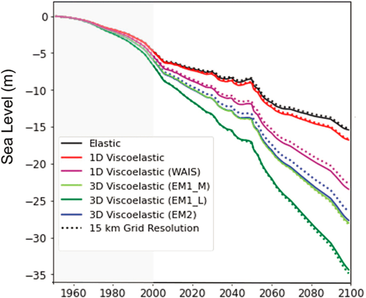
As the GIA uplifts sub-ice topography, it contributes to sea level fall at marine grounding lines. For example, when viscous deformation is not considered, models show up to 15 percent difference in ice loss over the last 25 years (Wan et al., 2022), and this difference increases to 60 percent when considering ice loss out to 2100. Book et al. (2022) argue that isostatic uplift may be enough to delay an unstable retreat of Thwaites Glacier. It is likely that viscous Earth deformation will slow marine ice sheet retreat, but retreat rates will be variable as they are influenced by bedrock topography and Earth structure, balanced against rates of ice loss. Additionally, because of the change of the Earth’s shape, GIA may have a far-field effect on the sea level (Woodward, 1888), significantly increasing sea level risk in regions of the Northern Hemisphere (Pan et al., 2021).
The study of the GIA is multidisciplinary and requires direct, long-term measurements of the Earth’s movement using GNSS. It also demands the use of sophisticated geodynamic simulations that take into consideration the 3D rheological properties of the Earth’s interior (Figure 3-9) and requires accurate knowledge of the internal thermal and rheological structures of the Earth. Over the past decade, studies have found that the viscosity of the uppermost mantle can range between orders of magnitude. East Antarctica is a craton20 with a very cold continental lithosphere (fast seismic velocities), whereas West Antarctica is underlain by hot upper mantle (slow seismic velocities). These velocities can be used to estimate mantle viscosities of West Antarctica of roughly 1018–1019 pascal-seconds (Figure 3-10; O’Donnell et al., 2017). According to these low viscosities, GIA should occur over a few hundred years, rather than thousands of years as was previously thought (van der Wal, 2022). Similarly, uplift rates from
___________________
20Cratons are the “stable interior portion of a continent characteristically composed of ancient crystalline basement rock” (Britannica Editors, 2017, para. 1).
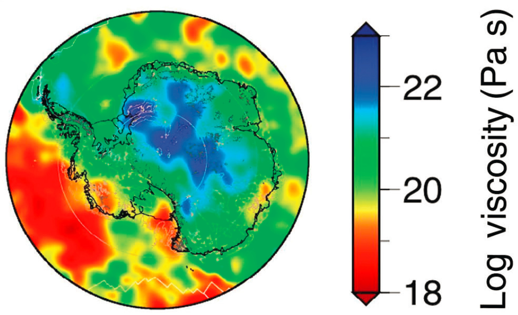
NOTE: High uplift rates have been observed in the low-viscosity regions in West Antarctica.
SOURCE: Used with permission of The Geological Society Publishing House from Ivins et al., 2023. Permission conveyed through Copyright Clearance Center, Inc.
GNSS receivers in West Antarctica deployed as part of the POLENET (Polar Earth Observing Network) project show GIA of less than 41 mm per year, which are some of the largest in the world (Barletta et al., 2018).
To improve mantle viscosity estimates, more dense networks of GNSS that monitor uplift rates in sensitive areas are needed, as well as improved imaging of the crust and uppermost mantle beneath the Antarctic coastal areas. Antarctica is surrounded by oceans where there are few seismometers, which limits mantle imaging resolution along the coastal and shelf regions and the far southern oceans around Antarctica (Figure 3-11). Better subsurface imaging would be enabled by a vessel that can deploy ocean-bottom seismometers and a vessel that can support helicopters to deliver seismic and GNSS instruments to coastal regions. Vessels outfitted with seismic systems for imaging the shallower structure, including airgun arrays and streamers, will also help reduce uncertainties.

NOTES: GAMSEIS = Gamburtsev Antarctic Mountains Seismic Experiment; GPS = global positioning system; iris-PERMANENT = Incorporated Research Institutions for Seismology; POLENET = Polar Earth Observing Network; RIS = Seismic Experiment on the Ross Ice Shelf; TAMNNET = Transantarctic Mountains Northern Network; TAMSEIS = Transantarctic Mountains Seismic Experiment; UK-ANET = U.K. Antarctic Network.
SOURCE: Weisen Shen.
CONCLUSIONS
Antarctica’s ice sheets, which contain approximately 58 m of sea level rise potential, may be approaching a dangerous tipping point toward major and potentially irreversible ice mass loss. Sea level rise due to greenhouse gas emissions will last centuries to millennia and affect the entire global community and economy, especially roughly 1 billion people who live in low-lying coastal zones. Oceanic forcing of the Antarctic ice sheets, through heat delivery and mechanical erosion, is expected to be the dominant source of ice mass loss in the next century, with atmospheric forcing also causing substantial ice mass loss. Major uncertainties remain about rates and extent of ocean warming, transport of heat through the sub–ice shelf cavities, and the sensitivity of the surface mass balance of ice sheets to increasing global temperatures.
Conclusion 3-1: Observations of surface energy, heat transport, and ice mass balance will result in better model representation of ice sheet flow and sensitivity to atmospheric and oceanic forcing, leading to improved projections of global and local rates of sea level rise.
Limited understanding of key processes, such as how grounding line retreat may trigger self-perpetuating feedbacks (e.g., marine ice sheet and ice cliff instability), results in uncertain projections of sea level rise. Constraining these processes through targeted observations and verifying models through paleoclimatic records will help clarify projections about how much and how fast the sea level will rise.
Conclusion 3-2: Increased remote and in situ observations of existing ice shelf cavities, grounding zones, and ice fracture mechanics, as well as more detailed reconstructions of the rates and regional extent of ice loss during past warm periods, will elucidate tipping points for possible irreversible ice mass loss.
Resolving uncertainties in sea level rise involves interdisciplinary research, particularly on ice–ocean interaction and the interaction of ice and ocean with the solid Earth and subglacial hydrology. Recent discoveries, including surprisingly rapid rates of uplift on the Antarctic Peninsula, suggest that extensive and robust monitoring of these processes may be needed for accurate predictions of sea level rise.
Conclusion 3-3: Improved observations and modeling of geologic and geophysical processes and properties—including glacial isostatic rebound; geothermal heat flow; subglacial geology and hydrology; and the seismic, thermal, and rheological properties of the underlying lithosphere–asthenosphere system—will improve accurate projections of sea level rise.
TABLE 3-1 Science Traceability Matrix
| Science Priority | Observations | Needed Capability |
|---|---|---|
| How much and how fast will ocean warming raise sea level? | Observations of temperature, speed, and salinity within ice shelf cavities | Ice shelf drilling, subshelf measurements, and long-term monitoring of temperature and salinity (e.g., cabled measurements), accessed via icebreaker and air support |
| Deployment of autonomous underwater vehicles (AUVs) to grounding zones | ||
| Ice shelf basal melt rates | Ground-based or airborne radar, including ApRES (autonomous phase-sensitive radio-echosounder) | |
| Monitoring freshwater discharge across the grounding zone and near the coast/ice shelf | Profiling floats, buoys, moorings, and underway measurements deployed from an icebreaker | |
| Passive seismometer arrays, ground penetration radars, and other geophysical sensors, accessed via icebreaker and air support |
| Science Priority | Observations | Needed Capability |
|---|---|---|
| How much and how fast will atmospheric warming melt Antarctic ice from above? | Better monitoring of weather for regional climate models | Expanded deployments of autonomous weather stations via icebreaker and air support |
| Repeat remote sensing of ice surface properties | ||
| Monitoring of icequakes and other events to evaluate brittle ice processes (e.g., fracturing) | Ice shelf and ocean-bottom seismometers and hydrophones, deployed from icebreaker and air support | |
| Observations of surface melt processes (e.g., hydrofracture) | Repeat remote sensing | |
| In situ observations of surface energy balance and surface hydrological processes | ||
| Reconstruction of ice dynamics, past snowfall rates, and variability in westerly wind strength | Shallow ice cores from coastal ice rises, accessed via icebreaker and air support | |
| Ice-penetrating radar sounding | ||
| Radar reflectometry | ||
| How will floating ice processes impact the rate of ice sheet loss? | In situ observations of surface energy balance and lateral heat fluxes | Satellite observations of supraglacial melt features and laser altimetry for shallow surface lake depths |
| Airborne observation for shallow radar sounding of surface and near-surface hydrology | ||
| Observations of ice loss processes on the continental shelf, along the ice shelf front and under the ice shelf | Global navigation satellite systems (GNSS) stations and wave buoys deployed from an icebreaker at the edge of ice shelves, within mélange, and on icebergs | |
| Ice-tethered platforms for ocean profiling beneath fast ice and ice shelves | ||
| Instrumented seals, profiling floats, moorings, mobile autonomous vehicles, and ship-based hydrographic surveys | ||
| Seafloor bathymetry and geology | Airborne gravity and magnetics measurements | |
| Icebreaker, with active-source seismic instrumentation, multibeam sonar, and sub-bottom profiling, that is capable of deploying ocean and seabed sensors | ||
| Autonomous vehicles for bathymetric mapping and sampling | ||
| Will grounding zone instabilities create tipping points of irreversible ice loss? | Better mapping and sampling of areas that could retreat | Ice-penetrating radar coverage, including swath radar mapping |
| Autonomous sensors and AUVs launched from an icebreaker, with scientific echosounders and other environmental sensing payloads | ||
| Coring or sediment drilling through ice bore holes, accessed via icebreaker and air support | ||
| Rates of change in paleoceanographic records | Improved sampling of ice-proximal sediment accumulations via icebreaker-based sediment coring and seafloor drilling | |
| Ice drilling for sub-ice marine sediments, enabled by icebreaker and air support | ||
| Icebreaker bathymetric mapping, multichannel seismic reflection, sub-bottom profiling |
| Science Priority | Observations | Needed Capability |
|---|---|---|
| Will geological and geophysical properties and processes exacerbate or moderate sea level rise? | Distribution and characteristics of sedimentary basins in Antarctica | Airborne gravity and magnetic field strength data |
| Icebreaker access and air support to the coast to deploy land-based seismic stations | ||
| Distribution of past and present subglacial hydrology | Seismic instrumentation (active and passive) deployed from icebreaker and air support | |
| Repeat airborne coherent ice-penetrating radar surveys | ||
| Icebreaker with multibeam mapping, side-scan sonar, and multichannel seismic systems | ||
| Geothermal heat flux | Direct measure of heat flows from icebreaker-hosted sediment coring and drilling boreholes | |
| Access to coastal regions for in situ geothermal heat flux measurements on land | ||
| Ice, rock, and sediment drilling capacity for in situ geothermal heat flux measurements, accessed via icebreaker and air support | ||
| Icebreaker capable of deploying ocean-bottom seismic sensors | ||
| Repeated airborne radar surveys, including coherent radar systems and passive airborne radiometer instruments | ||
| Rheological and viscosity models of the upper mantle | Icebreaker capable of deploying ocean-bottom seismic sensors | |
| Access to near-coastal regions via air support for geophysical deployment and geological sampling | ||
| Icebreaker outfitted with seismic systems (e.g., airgun arrays and streamers) | ||
| Geodetic measurements of the GIA-related basement movement | Access to near-coastal regions via air support for GNSS deployment | |
| Ocean-bottom GNSS development and deployment from icebreaker | ||
| Rigid inflatable boat access to islands in the Southern Ocean | ||
| Rheological and viscosity models of the upper mantle | Icebreaker capable of deploying ocean-bottom seismic sensors | |
| Access to near-coastal regions via air support for geophysical deployment and geological sampling | ||
| Icebreaker outfitted with seismic systems (e.g., airgun arrays and streamers) | ||
| Geodetic measurements of the GIA-related basement movement | Access to near-coastal regions via air support for GNSS deployment | |
| Ocean-bottom GNSS development and deployment from icebreaker | ||
| Rigid inflatable boat access to islands in the Southern Ocean |


