2020 Census Data Products: Demographic and Housing Characteristics File: Proceedings of a Workshop (2023)
Chapter: 4 Evaluation of the Demonstration Data on Age
4
Evaluation of the Demonstration Data on Age
SINGLE YEAR OF AGE
Sarah Radway (Tufts University) and Miranda Christ (Columbia University) presented their research using single year of age from the Census Bureau as a crucial variable to help schools estimate the number of incoming students. They acknowledged that census data contain sensitive information about children and their families, and there are legal mandates from Title 13 that census data cannot be personally identifiable. Thus, privacy is integral to understanding census participation rates.
Radway’s and Christ’s use case was for school planning, and they created a synthetic data set with 291 kindergarten-age students and their families using the method of Flaxman and Haddock.1 Radway stated that the utility of the data can be impacted in the process of deidentification. Accuracy of estimates is critical because it impacts funding decisions made by school districts—hiring teachers, expanding classroom space—so inaccurate data may lead to insufficient allocation of resources. The research question posed was, How do the deidentification methods of swapping and differential privacy impact granular data such as single year of age?
The central question was how to best balance data utility and privacy for the case of single year age of data. Radway acknowledged that, while the Census Bureau has made a choice to use differential privacy to meet this challenge, there has been significant criticism of differential privacy’s impact on data integrity. Several works have critiqued the ability of differential
___________________
1 Associated code is available at https://github.com/aflaxman/ppmf_12.2_reid
privacy to preserve data utility under different circumstances, including small population sizes and small demographic subgroups (National Congress of American Indians, 2019; Ruggles, 2019; Wezerek and Van Riper, 2020). Radway and Christ’s analysis compared swapping with differential privacy—based on the principles outlined for the Census Bureau’s approach—creating algorithms using synthetic data for eight different census tracts to achieve swapping and differential privacy.
After the data were run through swapping and differential privacy algorithms, comparisons were made between the deidentified and ground truth histograms with the mean absolute percentage error for eight census tracts of varying sizes from synthetic state data. For each age, the absolute difference was calculated and divided by the known ground truth count to get a percentage, which was then averaged across the three age ranges: (1) total population, (2) ages less than 18 years, and (3) ages 4–5 years.
Christ said that, in their analysis, as populations got larger, the error decreased and there was also less variation between parameter values. Using a gray box to depict the national estimated swap rate in their presentation, they found that the error of swapping is a bit high compared with the error of differential privacy at many of the epsilon values. Both mechanisms had higher error for smaller populations. For swapping, the accuracy was especially unpredictable between parameter values with fairly high variation. However, differential privacy performed a bit more predictably across different population sizes. Figure 4-1 shows the curves for total population and individual ages 4–5 years for both swapping and differential privacy, where swapping is more jagged and differential privacy is smoother with a more predictable relationship between utility and privacy.
Christ summarized that both mechanisms have higher error for smaller populations. Swapping accuracy varies more between parameter values. Differential privacy performs more predictably across different population sizes and provides a predictable relationship between utility and privacy. Christ stated that her research with Radway showed that both mechanisms were susceptible to error, but she concluded that the other properties of differential privacy make it more desirable. Christ acknowledged Steven M. Bellovin (Columbia University) for his help on this research.
Comparisons for Young Children
Another use case involving young children was presented by William O’Hare (consultant to the 2020 Census Count All Kids campaign), who expressed that young children, specifically ages 0–4 years, is an important age group to examine when considering the impact of differential privacy on children. He prefaced his comments by noting the net undercount for young children not only is severe but also has been worsening over the past
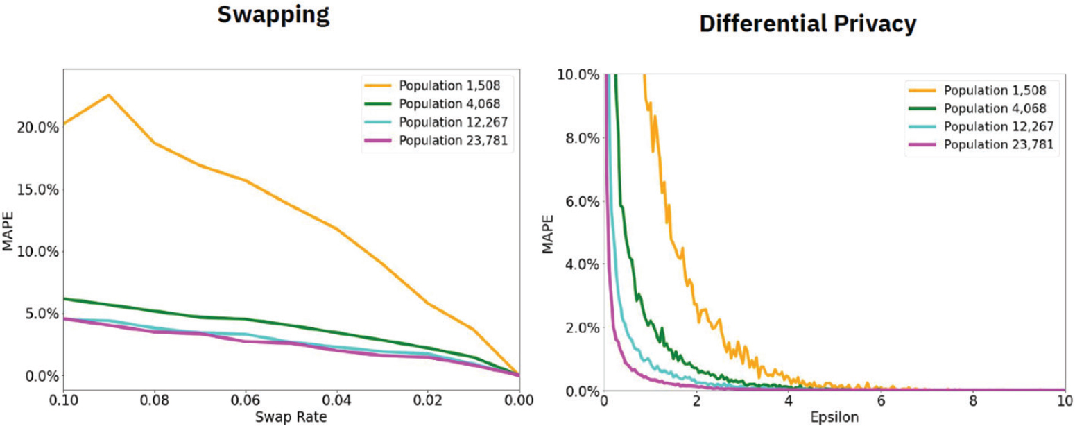
NOTE: MAPE = mean absolute percentage error.
SOURCE: Sarah Radway and Miranda Christ workshop presentation, June 21, 2022.
several decades, beginning in 1950. O’Hare stated the count of children has plummeted since 1980 and was 5.4 percent of the total in the 2020 Census, which is a more significant undercount than for any other age group in the census. He argued that an accurate count of young children is important not only for planning regarding child care and daycare, with preschool and elementary school on the horizon, but also because these children do not have voices of their own in the public arena.
O’Hare discussed Table 4-1 in his presentation about the absolute errors for the ages 0–4 years population in four geographic units, based on the demonstration data released in March 2022. Of the areas he analyzed (states, counties, school districts, and places), he cautioned that 302 counties are relatively small, with populations less than 5,000, for which differential privacy may be an issue. However, the error metrics, as measured by having absolute percent errors of five percent or more, were problematic for school districts (27% error) and places (39% error).
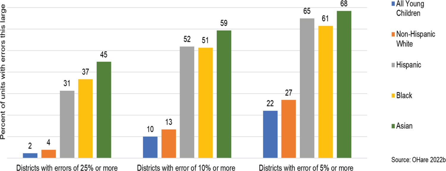
When looking at absolute percent errors in Figure 4-2 in school districts for children ages 0–4 years by race and Hispanic origin, O’Hare pointed out that the disparities between the percent error for non-Hispanic Whites compared with Hispanics and Black and Asian children were higher at each error level. He noted that greater than 60 percent of the school districts have errors of five percent or more for Hispanic, Black, and Asian young children. He observed that the errors are not distributed equally across the states. The implications of this research are that some superintendents will
| States | Countiesa | School Districts | Places | |
|---|---|---|---|---|
| Number of units in the analysis | 50 | 3,221 | 10,864 | 28,729 |
| Mean size of school district (Children ages 0–4 based on Summary File) | 39,873 | 6,342 | 1,880 | 546 |
| Mean absolute numeric error | 7 | 8 | 12 | 6 |
| Mean absolute percent error | Rounds to 0 | 0.9% | 4.3% | 13.6% |
| Percent of units with absolute errors of five or more young children | 58% | 62% | 69% | 46% |
| Percent of units with absolute percent errors of 5% of more | 0% | 3% | 27% | 39% |
a There are 302 counties with total population less than 5,000.
SOURCE: William O’Hare workshop presentation, June 21, 2022.
SOURCE: William O’Hare workshop presentation, June 21, 2022.
have large errors in their data for planning purposes, and these errors may also be tied to funding and other resources. O’Hare also raised equity issues in his analysis of children ages 0–4 years by questioning whether it is fair to inject differential privacy error into groups that already have a lot of error, such as young children, Hispanics, or Blacks.
The final issue O’Hare raised involved the processing of differential privacy; he used examples from the redistricting and Demographic and Housing Characteristics (DHC) files. He explained that before differential privacy was applied in 2010, there were 82 blocks with children 17 and under but no adults. However, this rose to 163,000 blocks after differential privacy was applied. O’Hare explained that the differential privacy algorithm independently injects noise for adults and children without accounting for adults who are parents of the children. The larger concern about such improbable results is that they damaged the Census Bureau’s credibility; these problems will extend to the American Community Survey if the same differential privacy method is applied to those data as well.
Using Age for City Services
Joel Alvarez and Erica Maurer (New York City Department of City Planning) examined the effect of disclosure avoidance noise on DHC age data and the allocation of city resources. Alvarez explained that their office works on demographics and is embedded within New York City’s planning agency, so they use census data on a daily basis to answer critical questions about the functioning of their city and to better plan for future needs. The questions that come to their office involve overall population counts and issues of racial equity, but sometimes inquiries are more nuanced and answers require characteristics and geographic detail that they used to obtain from the decennial Summary Files. Age is one of the most important characteristics, and these data can be critical in planning how to allocate resources to evacuate young and elderly populations, how the Department for the Aging can best plan in-home services, and how New York City can plan for the future by creating population projections using five-year cohort data.
In 2010, New York City had 2,168 tracts. Figure 4-3 shows analysis for one tract (Census Tract 450) around Ocean Parkway in central Brooklyn. This is a tract with a population just under 700 people. Comparing the five-year age cohorts with the three sets of demonstration data released to date (October 2019, May 2020, and March 2022), Alvarez stated the erratic data that were initially seen with differential privacy noise infusion improved with the most recent demonstration file. Alvarez stated he cannot definitively say which depiction is closer to reality because they do not have the Census Edited File (CEF), which is unaltered by any form of disclosure avoidance noise. The overall dissonance is gauged by absolute
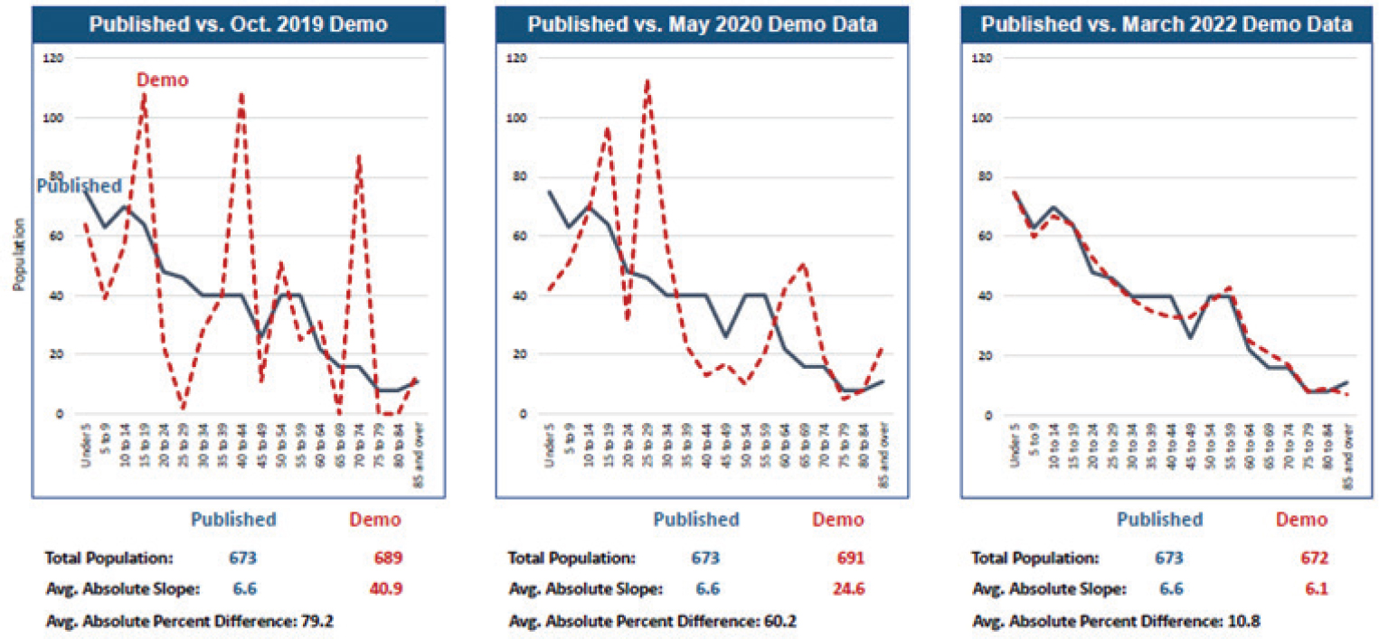
SOURCE: Joel Alvarez and Erica Maurer workshop presentation, June 22, 2022.
percent differences between demonstration files and 2010 published data. The absolute percent difference in the original demonstration was 79.2 percent; it declined to 60.2 percent with the May 2020 file and dropped to 10.8 percent with the March 2022 file. While improved for this small tract, Alvarez questioned whether the data are fit for use.
When extreme differences—defined as absolute differences of 10 percent or more—were compared across all tracts for all three demonstration files, the data demonstration file available at the time of the workshop (March 2022 file release) with a person-level privacy-loss budget of ε = 20.82 had substantially lower percentages of tracts with extreme differences across all age groups. However, Alvarez noted a pronounced jump in extreme difference in the March 2022 demonstration file for age groups 70 and over.
Extreme differences produced from the March 2022 demonstration file were found to be associated with relatively small counts. Greater than 90 percent of the tract-level extreme differences occur where an age group has a population count of under 200. Alvarez explained one solution is to aggregate census tracts. Over the past two decades, their office has developed and refined a new statistical geography called Neighborhood Tabulation Areas (NTAs). These are tract aggregations that approximate New York City neighborhoods with populations ranging from about 15,000 up to 100,000.
When the three iterations of demonstration files for extreme differences were analyzed, Alvarez and Maurer found that differences were essentially nonexistent at the NTA level in the March 2022 file, and extreme differences were found only for the 80–84 age group. A similar analysis, evaluating all three demonstration files, was also conducted for an individual NTA—Crown Heights South in central Brooklyn. The first demonstration file exhibited the most incongruities, and the final March 2022 file data were practically identical to the published Summary File 1 (SF1) data.
For the purposes of New York City, the latest March demonstration file represents significant improvement over the previous two files. However, users should be cognizant of the limitations of using five-year age-group data at the census tract level. Most of the New York City tracts had extreme deviations, so not all five-year age data are fit for use at this level. Alvarez suggested that the extreme differences between the 2022 demonstration data and published (SF1) data were rare for counts exceeding 200. Alvarez commented, “If users want to be sure to avoid extreme distortions, it is important to either collapse age groups or create tract aggregations.” He noted that as they moved up the geographic summary level, they found the noise was minimized and data were indeed fit for use.
This presentation concluded with observations about what is missing. Alvarez noted that the current DHC demonstration file lacks information about detailed race and ethnicity, and expressed concern about plans to
release detailed race and ethnicity only down to the county level. Detailed race and ethnicity were was previously available at the tract level, and the change seriously impacts their provision of services. Finally, Alvarez commented that the planned 2023 release of data is two years later than the comparable 2010 Census release. Each day stakeholders wait is another day they cannot use these data for decision-making, so he implored the Census Bureau to consider releasing the data in a segmented manner akin to what is planned for the Detailed DHC (DDHC) File.
AGE HEAPING
Ethan Sharygin2 (Portland State University) presented his analysis on age heaping—that is, when a reported age tends to be rounded and ends in a zero or five, which is known to occur in censuses (Arriaga, 1968). There are techniques from demography that are intended to smooth noisy age data (Currie et al., 2004; Dyrting, 2020).
Sharygin described analysis using DHC data for single year of age distribution for a small county where the female population is about 1,600. He described the 2010 SF1 as already exhibiting noise, and stated that the May 2020 demonstration data as seen in Figure 4-4 (shown in circles) were beyond what he felt he could use, with a massive amount of noise and outliers. Two smoothing nonparametric techniques—p-splines and the Tool for Population Analysis Using Linear Splines (P-TOPALS)—were compared for May 2020 and March 2022 data, which he demonstrated by plotting the data against the SF1 data for single-age distributions. Sharygin noted that the changes in the TopDown Algorithm (TDA) and the increased privacy-loss budget had good effects, and there were more improvements when using the two age-smoothing techniques.
Sharygin used the P-TOPALS age-smoothing technique to examine all U.S. counties, as shown in Figure 4-5. The black dots are the untreated estimates for age with error between the published SF1 and demonstration data, and the blue dots are the errors from the smoothed age distributions. When the 2022 data were compared with the 2020 demonstration data, the estimates improved across the board. Sharygin observed that the errors with the demonstration data were correlated with population size, and there were reliability problems with the differential privacy estimates for small- and medium-size areas. Specifically, more than a quarter of the counties in the United States had a coefficient of variation that exceeded what is considered usable from the census. Use of the smoothing technique led to meaningful improvement; accuracy improved for 90 percent of counties
___________________
2 Coauthors were Sigurd Dyting (Charles Darwin University) and Abraham Flaxman (University of Washington).
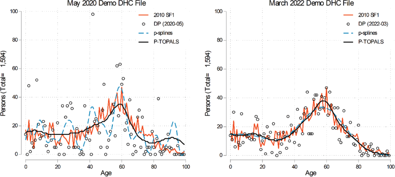
NOTE: DHC = Demographic and Housing Characteristics File; DP = differential privacy; P-TOPALS = Tool for Population Analysis Using Linear Splines; SF1 = Summary File 1.
SOURCE: Ethan Sharygin workshop presentation, June 21, 2022.
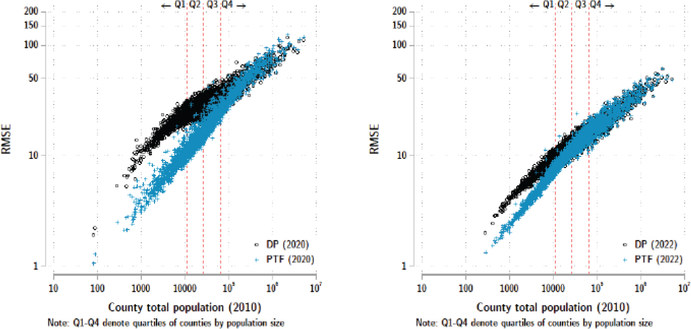
NOTE: DP = differential privacy; PTF = pedotransfer function; RMSE = root mean squared error.
SOURCE: Ethan Sharygin workshop presentation, June 21, 2022.
with 25,000 people or fewer and for 99.5 percent of counties with fewer than 10,000 residents.
Sharygin observed that the 2020 data using the TDA show significant improvements over time. However, measurement of characteristics of small areas or very small cross-sections of large-area populations remains problematic. When the data are aggregated, the errors diminish. He further commented that changes such as the higher privacy-loss budget and changes to the Gaussian noise mechanism had positive effects on fitness-for-use. He concluded by stating that the demonstration data could be further improved by smoothing age distributions to get results even closer to the published data without compromising the formal privacy guarantee that motivates use of the TDA.
DISCUSSION
A webinar attendee from Northwest University in South Africa posed a question regarding whether swapping and differential privacy algorithms could be adopted in other factors such as education, income, marital status, and place of reference. Radway responded that similar results were found when age, sex, and race were used as the basis for swapping (Christ et al., 2022).
Tom Mueller (University of Oklahoma) posed a related question to Radway and Christ regarding clarification on their swapping algorithm. He asked if they swapped only the higher-risk cases. Radway stated that they prioritized unique households first in terms of household age, sex, and race breakdown for members in an attempt to follow the same principles based on what is known about the TDA.
Webinar attendee Ryan McCammon (University of Michigan) placed a comment in the chat for those present in the workshop. As moderator, danah boyd (Microsoft Research) summarized the comment as a statement that swapping may have introduced uncertainty into prior data (e.g., 2010 block-level data for total population, total housing units, occupancy status, group-quarters counts), so problematizing the accuracy of all data under swapping is a bit disingenuous when the prior data are held invariant. boyd stated that it is important to recognize that when one thing is held invariant, more noise is created elsewhere to protect privacy. As boyd explained, the challenge is, “Where do we care about uncertainty?” She elaborated that the communication challenge frequently comes up with advocacy crowds, who claim, “Everything is always sunny in Suitland.” Radway agreed with boyd and added that one has to choose the variables to be prioritized. She emphasized the importance of choosing a constraint with the data.


