Pile Design for Downdrag: Examples and Supporting Materials (2024)
Chapter: Appendix D: Design Example 2 - Embankment Fill Over Clay Using PileAXL Program
APPENDIX D
Design Example 2 — Embankment Fill Over Clay Using PileAXL Program
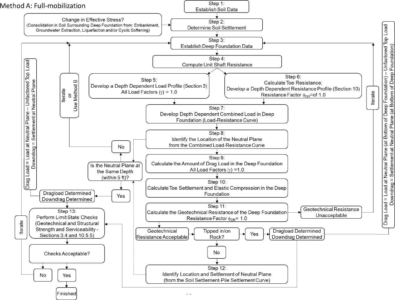
Design Example 2 is a continuation of Design Example 1. Like Design Example 1, the design data that were used for Design Example 2 were acquired from Briaud and Tucker (1997). Moreover, like Design Example 1, the focus of Design Example 2 was on determining the location of the neutral plane and magnitudes of the drag load and downdrag as demonstrated using 1) Load-Resistance profiles and 2) Pile-Soil Settlement profiles. Like Design Example 1, Design Example 2 uses Method A (full mobilization) proposed by the NCHRP 12-116A project team but uses software instead of hand calculations. In this design example, the Innovative Geotechnics PileAXL Version 2.4 (Innovative Geotechnics, 2023a) software program was used to certify the results from the hand calculations that were performed in Design Example 1. The proposed NCHRP12-116A flowchart steps were followed to complete the design example.
Step 1: Establish soil data
Determine the geotechnical engineering design parameters and establish a profile of the soil deposit. Index parameters

Table D1. Briaud and Tucker (1997) Example Problem 1 PILENEG Program input data.
| Pile Material | Concrete |
| Pile Shape | Octagonal |
| Pile Face [mm] | 174* |
| Pile Perimeter [m] | 1.39 |
| Pile Area [m2] | 0.145 |
| Pile Embedded Length [m] | 41.76 |
| Pile Modulus [kN/m2] | 2.41 x 10⁷ |
| Top Load on Pile [kN] | 2225 |
| Number of Pile Increments | 50 |
| Soil Young’s Modulus [kN/m2] | 21531 |
| Soil Poisson’s Ratio | 0.3 |
| Soil Ultimate Bearing Capacity [kN/m2] | 7097 |
| Ground Wateryable Depth [m] | 0* |
| * Inferred or interpolated parameters using correlations contained in Briaud and Tucker (1997). | |
(water content, Atterberg limits, unit weight) should be used to help identify the stratigraphy of the soil deposit. The relevant soil data that are needed include soil shear strength and total unit weight. An example of the soil stratigraphy for the Briaud and Tucker (1997) Example Problem 1 design example is included as Figure D1.
The soil modulus (M) presented in Figure D1 was calculated using Equation 1 based on the Young’s modulus (E) and Poisson’s ratio (ν) values that were provided in Briaud and Tucker (1997). The undrained shear strength values were determined by converting the provided Briaud and Tucker (1997) friction data to undrained shear strength data (Figure D2).
| Eqn. 1 |
Step 2: Determine soil settlement
The amount of expected soil settlement was determined using consolidation theory. The calculations performed to determine the amount of soil settlement resulting from the embankment fill being placed were identical to the calculations performed in Step 2 of Design Example 1. The obtained soil settlement profile is provided as Figure D3.

Step 3: Establish pile data
The pile data required to determine the drag load and downdrag include 1) the side resistance acting on the pile(s), 2) the end bearing resistance provided by the pile(s), 3) the unfactored pile head deadload(s), and 4) the elastic compression of the pile(s). Multiple pile types or pile geometries may be considered to determine the magnitude of downdrag/drag load on the pile(s). To compute the drag load for a given design scenario, the following pile data are required: pile material, pile diameter or pile perimeter, and pile modulus. The pile considered for this design example was an octagonal pile; the distance across the pile (0.4195m) was used as the pile diameter within the PileAXL software program. As shown in Figure D4, the section type, diameter, cross-sectional area (0.145m2), and pile modulus (2.41x10⁷ kN/m2) were input into the Pile AXL software program using the Define – Pile Sections pop-out window.

Step 4: Compute incremental side resistance
For a given pile geometry (diameter, length), the side resistance was determined for discretized intervals. Using the Define – Analysis Option popout window (Figure D5), the pile length (41.76m), and number of pile increments (50) were entered.


The design code to be used for the computations was also selected in the Analysis Option window using the toggle switches in the Pile Capacity Design Code section. The Working Load Design Approach was selected for use for this design example. In addition to selecting the Working Load Design Approach option in the Analysis Option window, the partial factors of safety for side resistance, base resistance, total resistance, and tensile resistance were each set to unity (Figure D6) using the Define – Design Approach window.

The three soil materials chosen for the design example were entered using the Define – Soil Materials window (Figure D7). Each material was first created using the New tab, and then the parameters for each soil material were modified using the Edit tab (Figure D8). The material type (cohesive) and material name (API Clay), and total unit weight (19.5kN/m3) were selected for each soil material. The undrained shear strength values that were previously shown in Figure D1 were input by listing the undrained shear strength at the top of the layer and the rate of change in undrained shear strength as a function of depth within the layer (0.787kPa/m for API Clay 1, 5.130 kPa/m for API Clay 2, and 0.000 kPa/m for API Clay 3).

Each of the aforementioned soil materials was then applied to respective layers using the Define – Soil Layers pop-out window (Figure D9). The depths for each of the layers were established following Figure D1. The depth to the water table of 0.00m was also established. By selecting one of the Edit tabs under the Advanced Input column within the Define – Soil Layers pop-out window, the T-Z and Q-Z parameters were input (Figure D10). The T-Z Curve Model, API Residual Ratio, and Q-Z Curve Model were set to T-Z Curve - API Clay, 0.9, and Q-Z Curve - API Clay, respectively. The
limiting values of ultimate shaft resistance (fs-max) and ultimate end bearing resistance (fb-max) were computed using the undrained shear strength (su) for each layer and the vertical effective stress at the top and bottom of each layer. Specifically, the equations prescribed in the PileAXL users manual (Innovative Geotechnics, 2023b), presented herein as Equations 2 through 6, were used.
| Eqn. 2 |
| Eqn. 3 |
| Eqn. 4 |
| Eqn. 5 |
| Eqn. 6 |
Note: α,ψ = computation parameters


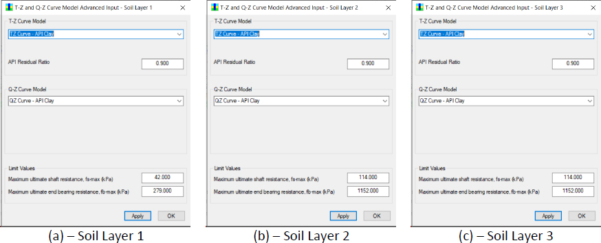
Table D2. Parameters used in Define – Soil Layers – Edit window.
| z | su | σz,o′ | ψ | α | fs | fb |
| [m] | [kPa] | [kPa] | [rad] | [rad] | [kPa] | [kPa] |
| 0.00 | 13 | 0.00 | 13415.89 | 0.05 | 1 | 117 |
| 22.86 | 31 | 221.51 | 0.14 | 1.34 | 42 | 279 |
| 41.76 | 128 | 404.65 | 0.32 | 0.89 | 114 | 1152 |
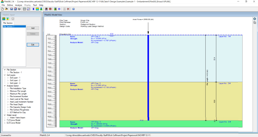
The calculated values obtained from Equations 2 through 6 are presented in Table D2. These values were also the values of fs-max and fb-max shown as the limiting values in Figure D10. The completed input, as shown in the main window prior to analyzing the data, is shown in Figure D11. The Analyze button was then selected and the output Unit Side Resistance (ULS fs), Ultimate Total Shaft Resistance (ULS Qs), and Ultimate Bearing Resistance (ULS Qb) results are presented in graphical form in the top right of the output window. The data were also presented in tabular form below the aforementioned plots within the PileAXL output window (Figure D12). The first (Depth), third (ULS Qs), fourth (ULS Qb), and fifth (Qult) columns of data from the PileAXL Output were then copied into Microsoft Excel for further processing (Table D3).
Step 5: Develop a depth-dependent load profile
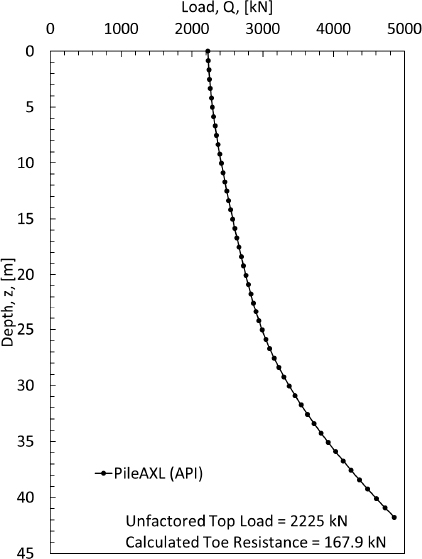
The depth-varying load profile was developed by first determining the cumulative load in the pile, as a function of depth (Qi), by adding the unfactored top load (UTL=2225kN from Briaud and Tucker, 1997) to each of the ULS Qs values (Equation 7). The axial force of (2550kN) that is shown in Figure D11 was used to generate the complete load-settlement curve for this pile (full mobilization) but not used as the unfactored top load. This 2550kN of axial force (shown in Figure D11) should not be used as the unfactored top load for the aforementioned calculations. More information about the use of the 2550kN for axial force is provided later in Step 11. Therefore, at a depth of 0m, the load in the pile was equal to the unfactored top load (2225kN). The depth-varying load profile is summarized in Table D3 and presented in Figure D13.
| Eqn. 7 |

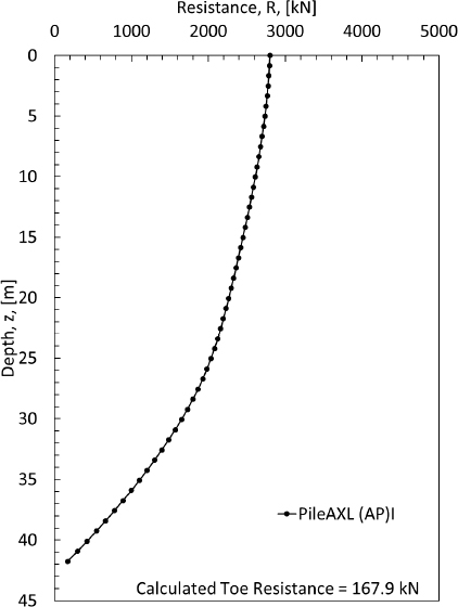
Step 6: Calculate end bearing resistance and develop the depth-dependent resistance profile
To develop the depth-varying resistance profile, incremental side resistance (∆Qi) values were calculated from the output results from the PileAXL software program. For the first depth increment, the incremental side resistance (∆Qi=1) was obtained by subtracting the ULS Qs value in the first row of data (ULS Qsi=1) from the ULS Qs value in the second row of data (ULS Qsi=2). This discretization process continued row by row from the top of the pile to the bottom of the pile (from j=2 to j=n). The resistance profile was then developed through accumulation of the ∆Qi values from the bottom of the pile to the top of the pile. The resistance value at the bottom of the pile was the summation of the end bearing resistance (Qbmax) and the incremental side resistance (∆Qi). Therefore, each resistance value included the end bearing resistance at the tip of the pile (Qbmax) and the summation of the incremental side resistance from the tip of the pile to the depth interval for which calculations were being performed. For the clay profile that was investigated, the end bearing resistance at the tip of the pile (Rb) was calculated using the undrained shear strength at the tip of the pile (su) and the cross-sectional area at the end of the pile (At) as obtained from Equations 9 and 10. The calculated resistance profile (Ri), for the octagonal precast concrete pile as calculated using Equation 11, is included in Table D3 and shown in Figure D14. The minimum Q and R values for each depth are also reported in Table D3.
| Eqn. 8 |
| Eqn. 9 |
| Eqn. 10 |
| Eqn. 11 |
Table D3. Useful PileAXL output and corresponding calculated values using Microsoft Excel.
| Depth | ULS fs | ULS Qs | ULS Qb | Qult | ∆Q | Q | R | min(Q,R) | Comments: ULS fs = Ultimate unit side resistance (PileAXL output), |
| [m] | [kPa] | [kN] | [kN] | [kN] | [kN] | [kN] | [kN] | [kN] | |
| 0.000 | 2.879 | 0.000 | 17.057 | 17.057 | 5.132 | 2225.000 | 2800.163 | 2225.000 | |
| 0.835 | 5.962 | 5.132 | 17.920 | 23.052 | 7.836 | 2230.132 | 2795.031 | 2230.132 | |
| 1.670 | 7.536 | 12.968 | 18.783 | 31.750 | 9.854 | 2237.968 | 2787.196 | 2237.968 | |
| 2.506 | 9.439 | 22.822 | 19.646 | 42.467 | 11.944 | 2247.822 | 2777.342 | 2247.822 | |
| 3.341 | 11.136 | 34.766 | 20.509 | 55.275 | 13.843 | 2259.766 | 2765.397 | 2259.766 | |
| 4.176 | 12.710 | 48.609 | 21.371 | 69.981 | 15.622 | 2273.609 | 2751.554 | 2273.609 | |
| 5.011 | 14.202 | 64.231 | 22.234 | 86.466 | 17.320 | 2289.231 | 2735.932 | 2289.231 | |
| 5.846 | 15.634 | 81.551 | 23.097 | 104.648 | 18.958 | 2306.551 | 2718.612 | 2306.551 | |
| 6.682 | 17.023 | 100.509 | 23.960 | 124.469 | 20.550 | 2325.509 | 2699.654 | 2325.509 | |
| 7.517 | 18.378 | 121.059 | 24.823 | 145.882 | 22.033 | 2346.059 | 2679.104 | 2346.059 | |
| 8.352 | 19.576 | 143.092 | 25.686 | 168.778 | 23.110 | 2368.092 | 2657.071 | 2368.092 | |
| 9.187 | 20.234 | 166.202 | 26.549 | 192.751 | 23.874 | 2391.202 | 2633.961 | 2391.202 | |
| 10.022 | 20.892 | 190.076 | 27.412 | 217.487 | 24.637 | 2415.076 | 2610.088 | 2415.076 | |
| 10.858 | 21.549 | 214.713 | 28.274 | 242.987 | 25.401 | 2439.713 | 2585.45 | 2439.713 | |
| 11.693 | 22.207 | 240.114 | 29.137 | 269.251 | 26.164 | 2465.114 | 2560.05 | 2465.114 | |
| 12.528 | 22.865 | 266.278 | 30.000 | 296.278 | 26.928 | 2491.278 | 2533.885 | 2491.278 | |
| 13.363 | 23.522 | 293.206 | 30.863 | 324.069 | 27.691 | 2518.206 | 2506.958 | 2506.958 | |
| 14.198 | 24.180 | 320.897 | 31.726 | 352.623 | 28.455 | 2545.897 | 2479.266 | 2479.266 | |
| 15.034 | 24.838 | 349.352 | 32.589 | 381.941 | 29.218 | 2574.352 | 2450.812 | 2450.812 | |
| 15.869 | 25.495 | 378.570 | 33.452 | 412.022 | 29.982 | 2603.570 | 2421.593 | 2421.593 | |
| 16.704 | 26.153 | 408.552 | 34.315 | 442.867 | 30.745 | 2633.552 | 2391.611 | 2391.611 | |
| 17.539 | 26.810 | 439.298 | 35.177 | 474.475 | 31.509 | 2664.298 | 2360.866 | 2360.866 | |
| 18.374 | 27.468 | 470.806 | 36.040 | 506.847 | 32.272 | 2695.806 | 2329.357 | 2329.357 | |
| 19.210 | 28.126 | 503.079 | 36.903 | 539.982 | 33.036 | 2728.079 | 2297.085 | 2297.085 | |
| 20.045 | 28.783 | 536.115 | 37.766 | 573.881 | 33.800 | 2761.115 | 2264.049 | 2264.049 | |
| 20.880 | 29.441 | 569.914 | 38.629 | 608.543 | 34.563 | 2794.914 | 2230.249 | 2230.249 | |
| 21.715 | 30.099 | 604.477 | 39.492 | 643.969 | 35.327 | 2829.477 | 2195.686 | 2195.686 | |
| 22.550 | 30.756 | 639.804 | 40.355 | 680.159 | 37.415 | 2864.804 | 2160.359 | 2160.359 | |
| 23.386 | 33.696 | 677.219 | 44.212 | 721.431 | 41.609 | 2902.219 | 2122.944 | 2122.944 | |
| 24.221 | 37.981 | 718.828 | 49.834 | 768.662 | 46.584 | 2943.828 | 2081.335 | 2081.335 | |
| 25.056 | 42.266 | 765.412 | 55.456 | 820.867 | 51.558 | 2990.412 | 2034.752 | 2034.752 | |
| 25.891 | 46.550 | 816.970 | 61.078 | 878.047 | 56.532 | 3041.970 | 1983.194 | 1983.194 | |
| 26.726 | 50.835 | 873.502 | 66.699 | 940.201 | 61.507 | 3098.502 | 1926.661 | 1926.661 | |
| 27.562 | 55.119 | 935.009 | 72.321 | 1007.330 | 66.481 | 3160.009 | 1865.155 | 1865.155 | |
| 28.397 | 59.404 | 1001.490 | 77.943 | 1079.433 | 71.456 | 3226.490 | 1798.673 | 1798.673 | |
| 29.232 | 63.688 | 1072.946 | 83.564 | 1156.510 | 76.430 | 3297.946 | 1727.218 | 1727.218 | |
| 30.067 | 67.973 | 1149.376 | 89.186 | 1238.562 | 81.405 | 3374.376 | 1650.787 | 1650.787 | |
| 30.902 | 72.258 | 1230.781 | 94.808 | 1325.588 | 86.039 | 3455.781 | 1569.383 | 1569.383 | |
| 31.738 | 75.957 | 1316.820 | 100.429 | 1417.250 | 89.997 | 3541.820 | 1483.343 | 1483.343 | |
| 32.573 | 79.075 | 1406.817 | 106.051 | 1512.868 | 93.608 | 3631.817 | 1393.346 | 1393.346 | |
| 33.408 | 82.177 | 1500.425 | 111.673 | 1612.097 | 97.202 | 3725.425 | 1299.739 | 1299.739 | |
| 34.243 | 85.266 | 1597.626 | 117.295 | 1714.921 | 100.782 | 3822.626 | 1202.537 | 1202.537 | |
| 35.078 | 88.344 | 1698.408 | 122.916 | 1821.324 | 104.349 | 3923.408 | 1101.755 | 1101.755 | |
| 35.914 | 91.411 | 1802.757 | 128.538 | 1931.295 | 107.904 | 4027.757 | 997.4067 | 997.4067 | |
| 36.749 | 94.468 | 1910.660 | 134.160 | 2044.820 | 111.448 | 4135.660 | 889.5031 | 889.5031 | |
| 37.584 | 97.516 | 2022.108 | 139.781 | 2161.890 | 114.983 | 4247.108 | 778.055 | 778.055 | |
| 38.419 | 100.557 | 2137.091 | 145.403 | 2282.494 | 118.509 | 4362.091 | 663.0722 | 663.0722 | |
| 39.254 | 103.591 | 2255.600 | 151.025 | 2406.625 | 122.027 | 4480.600 | 544.5633 | 544.5633 | |
| 40.090 | 106.617 | 2377.627 | 156.647 | 2534.273 | 125.538 | 4602.627 | 422.5365 | 422.5365 | |
| 40.925 | 109.638 | 2503.164 | 162.268 | 2665.433 | 129.053 | 4728.164 | 296.9989 | 296.9989 | |
| 41.760 | 112.672 | 2632.217 | 167.946 | 2800.163 | - | 4857.217 | 167.9464 | 167.9464 |
Step 7: Develop the depth-dependent combined load profile for the pile
The combined load and resistance profile graph for the pile analyzed in the example presented herein is presented in Figure D15. The combined load plot begins at the top of the pile and follows the load curve until the intersection with the resistance curve then follows the resistance curve until the toe of the pile is reached. The combined profile includes the application of the unfactored top load on the pile and the end bearing resistance at the toe of the pile.
Step 8: Identify the location of the neutral plane from the combined load and resistance curve
The neutral plane is located at the intersection of the load and resistance curves when plotted on the same graph. The neutral plane was located at 13.68m based on the calculations that were performed (Figure D16). The maximum load in the pile, at the location of the neutral plane, was 2507kN.
Step 9: Calculate the amount of drag load in the pile
The amount of drag load in the pile is equal to the amount of load in the pile at the location of the neutral plane minus the amount of unfactored load applied to the top of pile. Based on the calculations, the drag load was determined to be 282kN. The drag load for the octagonal precast concrete pile is shown in Figure D16.


Step 10: Calculate toe settlement and elastic compression in the pile
The elastic compression (δEC) for each segment of the pile was calculated using 1) the load within the pile (Q above the neutral plane and R below the neutral plane, from Figure D15 shown previously), 2) the cross-sectional area of the pile (A), 3) the elastic modulus of the pile (E), and 4) the segmental length of the pile (Ls). Specifically, the elastic compression for each segment (δEC,s) of the pile was determined using Equation 12. The cumulative elastic compression in the pile was then determined by accumulating each of the elastic compression values from the bottom of the pile to the top of the pile (Equation 13). The calculated segmental and cumulative elastic compression values are tabulated in Table D4 and shown in Figure D17.
| Eqn. 12 |
| Eqn. 13 |
Table D4. Calculated elastic compression values.
| z | δEC,s | δEC | Comments: z=depth, Q=load, R=resistance, δEC,s=segmental elastic compression (from bottom to top), δEC=cumulative elastic compression, A=pile cross-sectional area=0.145[m2] Ep=pile elastic modulus=2.41E+07[kPa] Ls=length of each pile segment=0.8532[m] | |
| [m] | [kN] | [m] | [m] | |
| 0.000 | 2225.000 | - | - | |
| 0.835 | 2230.132 | 0.00053 | 0.02227 | |
| 1.670 | 2237.968 | 0.00053 | 0.02174 | |
| 2.506 | 2247.822 | 0.00054 | 0.02120 | |
| 3.341 | 2259.766 | 0.00054 | 0.02066 | |
| 4.176 | 2273.609 | 0.00054 | 0.02012 | |
| 5.011 | 2289.231 | 0.00055 | 0.01958 | |
| 5.846 | 2306.551 | 0.00055 | 0.01903 | |
| 6.682 | 2325.509 | 0.00056 | 0.01848 | |
| 7.517 | 2346.059 | 0.00056 | 0.01793 | |
| 8.352 | 2368.092 | 0.00057 | 0.01737 | |
| 9.187 | 2391.202 | 0.00057 | 0.01680 | |
| 10.022 | 2415.076 | 0.00058 | 0.01623 | |
| 10.858 | 2439.713 | 0.00058 | 0.01565 | |
| 11.693 | 2465.114 | 0.00059 | 0.01507 | |
| 12.528 | 2491.278 | 0.00060 | 0.01448 | |
| 13.363 | 2506.958 | 0.00060 | 0.01388 | |
| 14.198 | 2479.266 | 0.00059 | 0.01328 | |
| 15.034 | 2450.812 | 0.00059 | 0.01269 | |
| 15.869 | 2421.593 | 0.00058 | 0.01211 | |
| 16.704 | 2391.611 | 0.00057 | 0.01153 | |
| 17.539 | 2360.866 | 0.00056 | 0.01096 | |
| 18.374 | 2329.357 | 0.00056 | 0.01039 | |
| 19.210 | 2297.085 | 0.00055 | 0.00983 | |
| 20.045 | 2264.049 | 0.00054 | 0.00929 | |
| 20.880 | 2230.249 | 0.00053 | 0.00874 | |
| 21.715 | 2195.686 | 0.00052 | 0.00821 | |
| 22.550 | 2160.359 | 0.00052 | 0.00769 | |
| 23.386 | 2122.944 | 0.00051 | 0.00717 | |
| 24.221 | 2081.335 | 0.00050 | 0.00666 | |
| 25.056 | 2034.752 | 0.00049 | 0.00617 | |
| 25.891 | 1983.194 | 0.00047 | 0.00568 | |
| 26.726 | 1926.661 | 0.00046 | 0.00521 | |
| 27.562 | 1865.155 | 0.00045 | 0.00474 | |
| 28.397 | 1798.673 | 0.00043 | 0.00430 | |
| 29.232 | 1727.218 | 0.00041 | 0.00387 | |
| 30.067 | 1650.787 | 0.00039 | 0.00346 | |
| 30.902 | 1569.383 | 0.00038 | 0.00306 | |
| 31.738 | 1483.343 | 0.00035 | 0.00269 | |
| 32.573 | 1393.346 | 0.00033 | 0.00233 | |
| 33.408 | 1299.739 | 0.00031 | 0.00200 | |
| 34.243 | 1202.537 | 0.00029 | 0.00169 | |
| 35.078 | 1101.755 | 0.00026 | 0.00140 | |
| 35.914 | 997.4067 | 0.00024 | 0.00114 | |
| 36.749 | 889.5031 | 0.00021 | 0.00090 | |
| 37.584 | 778.055 | 0.00019 | 0.00069 | |
| 38.419 | 663.0722 | 0.00016 | 0.00050 | |
| 39.254 | 544.5633 | 0.00013 | 0.00034 | |
| 40.090 | 422.5365 | 0.00010 | 0.00021 | |
| 40.925 | 296.9989 | 0.00007 | 0.00011 | |
| 41.760 | 167.9464 | 0.00004 | 0.00004 |

Step 11: Compute the geotechnical resistance of the pile
The nominal compression resistance of the pile was determined using the Davisson Method (Davisson, 1972). Typically, the Davisson Method is intended to be used to determine the nominal axial downward resistance based on a measured load-displacement curve from a full-scale load test performed on a pile. However, a full-scale load test is not typically collected prior to commencement of fieldwork or production installation. To overcome a lack of data, a predicted load-displacement curve can be calculated using the PileAXL software program. A load-displacement curve should be used to estimate the location of the neutral plane, in addition to the neutral plane determined from the combined load-resistance profile graph. Data for the predicted curve were obtained by setting the axial force to 2550 kN, as discussed previously and shown previously in Figure D11. The axial force (shown previously in Figure D5) was set in the Define – Analysis Option pop-out window and was set in the Settlement Analysis - Axial Loading for Settlement input box. The axial force must be set to the largest value possible to generate a curve within the program. If the axial force is set too high for a given pile length, an error will be shown in the program (Figure D18) after selecting on Tools – Pile Settlement Results in the PileAXL Output window.

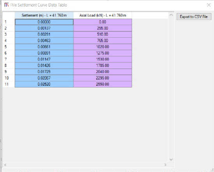
The load-displacement curve for the tip of the pile was desired; this curve was obtained by first selecting Pile Length = 41.760 (m) checkbox within the Define pile lengths for settlement analysis tab in the Define – Analysis Option window (Figure D19). With an appropriate axial load selected (2550 kN), a load-settlement curve (Figure D20) was obtained through Tools – Pile Settlement Results in the PileAXL Output window. Note: the PileAXL Output window did not appear until after the Analyze button was selected, the analysis was completed, and the Output window was displayed. After the PileAXL Output was displayed, the original main program window was locked for editing. The data in the “Pile Settlement curve plot for selected pile length” were obtained by right-clicking on the plot and then selecting Table. The load-settlement data were exported to a CSV file using the Export to CSV File tab (Figure D21). The PileAXL data are plotted along with the failure curve developed following the Davisson (1972) method. An additional data point was added to the PileAXL data due to the PileAXL curve not reaching the Davisson (1972) failure curve. The load for the additional
point was taken as the maximum ultimate resistance (Qult=2800.16kN) from Table D3 (as shown previously). This value was then placed into the Davisson (1972) equation to determine the corresponding settlement (0.041m). The predicted top-down load-settlement curve is presented as Figure D22. This pile is not tipped in rock, so Step 12 is initiated in the flow chart.


Step 12: Identify the location of and settlement at the neutral plane (from the soil settlement-pilesettlement curve)
When using the soil settlement-pile settlement graph, the neutral plane was located at the intersection of the soil settlement and pile settlement curves when plotted on the same graph as a function of depth. The pile settlement was obtained by adding the toe settlement (0.041m) that was previously reported in Figure D22 with the elastic compression as a function of depth that was previously reported in Figure D17. These values are shown in Figure D22 and tabulated in Table D5. As shown in Figure D23, the neutral plane was located at a depth of 12.11m. The amount of settlement at the neutral plane (also known as the downdrag) was identified to be 0.055m.
Following Step 12, the location of the neutral plane as obtained from the soil settlement-pile settlement curve (Step 12) and the location of the neutral plane as obtained from the combined load-resistance curve (Step 8) were compared. A depth of 12.11m was obtained from Step 12 and a depth of 13.36m was obtained from Step 8. This 1.25m (4.1ft) difference was less than the threshold 5ft difference. Therefore, the location of the neutral plane was selected as 13.36m because the location of the neutral plane from the combined load-settlement curve has less ambiguity than the location of the neutral plane from the soil settlement-pile settlement curve.
Step 13: Perform limit state checks
Limit state checks were performed to determine if the pile size was suitable for the design loads. For the structural strength limit state, the determined drag load (282kN) was multiplied by the drag load factor (γDR=1.1) to obtain a factored load of drag load 310kN. The unfactored top load (2225kN) placed on the top of the pile was multiplied by the deadload factor (γD=1.25) to obtain a factored deadload of 2781kN. The combined total factored load was 3091kN. The concrete compressive strength for the pre-stressed concrete pile was assumed to be 5000psi (34474kPa) resulting in a factored structural stress of 25856kPa (0.75*34474kPa) and a factored structural strength of 3749kN when the stress was multiplied by the cross-sectional area of the pile (0.145m2). If a concrete compressive strength of 5000psi (34474kPa), was used for the pre-stressed pile then the pile is adequately sized because the factored structural strength (3749kN) was determined to be greater than the combined total factored load (3091kN). If a concrete compressive strength less than 5000psi (34474kPa) was used for the pre-stressed concrete pile, then the pile would need to be larger in cross-sectional area or lengthened. Either modification to the pile would result in a change in the amount of drag load on the pile; Steps 3 through 13 of the NCHRP12-116A flowchart would need to be repeated to ensure the factored structural strength was greater than the total factored load.
Conclusion:
A design software program (Innovative Geotechnics PileAXL) was used to perform calculations to determine the amount of drag load and downdrag on a pile being subjected to a change in effective stress from an embankment. Using the flowchart developed during the NCHRP 12-116A project, the downdrag, drag load, and location of the neutral plane were determined to be 0.055m, 282kN, and 13.36m, respectively. If the compressive strength of the concrete in the pile was 5000psi (34474kPa), the pile was determined to be adequately sized to support the loading conditions applied to the pile.

Table D5. Soil settlement and pile settlement as a function of depth.
| zp | δp | Zs | δs | Comments: zp=depth for pile calculations, zs=depth for pile calculations, δp=pile settlement, δs=soil settlement. |
| [m] | [m] | [m] | [m] | |
| 0.000 | 0.0632 | 0.4176 | 0.0972 | |
| 0.835 | 0.0627 | 1.2528 | 0.0939 | |
| 1.670 | 0.0622 | 2.088 | 0.0905 | |
| 2.506 | 0.0616 | 2.9232 | 0.0872 | |
| 3.341 | 0.0611 | 3.7584 | 0.0839 | |
| 4.176 | 0.0605 | 4.5936 | 0.0806 | |
| 5.011 | 0.0600 | 5.4288 | 0.0774 | |
| 5.846 | 0.0594 | 6.264 | 0.0743 | |
| 6.682 | 0.0589 | 7.0992 | 0.0713 | |
| 7.517 | 0.0583 | 7.9344 | 0.0684 | |
| 8.352 | 0.0578 | 8.7696 | 0.0655 | |
| 9.187 | 0.0572 | 9.6048 | 0.0628 | |
| 10.022 | 0.0566 | 10.44 | 0.0601 | |
| 10.858 | 0.0560 | 11.2752 | 0.0575 | |
| 11.693 | 0.0554 | 12.1104 | 0.0550 | |
| 12.528 | 0.0548 | 12.9456 | 0.0526 | |
| 13.363 | 0.0542 | 13.7808 | 0.0503 | |
| 14.198 | 0.0536 | 14.616 | 0.0480 | |
| 15.034 | 0.0531 | 15.4512 | 0.0458 | |
| 15.869 | 0.0525 | 16.2864 | 0.0437 | |
| 16.704 | 0.0519 | 17.1216 | 0.0417 | |
| 17.539 | 0.0513 | 17.9568 | 0.0397 | |
| 18.374 | 0.0508 | 18.792 | 0.0378 | |
| 19.210 | 0.0502 | 19.6272 | 0.0359 | |
| 20.045 | 0.0497 | 20.4624 | 0.0341 | |
| 20.880 | 0.0492 | 21.2976 | 0.0323 | |
| 21.715 | 0.0486 | 22.1328 | 0.0306 | |
| 22.550 | 0.0481 | 22.968 | 0.0289 | |
| 23.386 | 0.0476 | 23.8032 | 0.0273 | |
| 24.221 | 0.0471 | 24.6384 | 0.0257 | |
| 25.056 | 0.0466 | 25.4736 | 0.0242 | |
| 25.891 | 0.0462 | 26.3088 | 0.0227 | |
| 26.726 | 0.0457 | 27.144 | 0.0213 | |
| 27.562 | 0.0453 | 27.9792 | 0.0198 | |
| 28.397 | 0.0448 | 28.8144 | 0.0185 | |
| 29.232 | 0.0444 | 29.6496 | 0.0171 | |
| 30.067 | 0.0440 | 30.4848 | 0.0158 | |
| 30.902 | 0.0436 | 31.32 | 0.0145 | |
| 31.738 | 0.0433 | 32.1552 | 0.0132 | |
| 32.573 | 0.0430 | 32.9904 | 0.0120 | |
| 33.408 | 0.0426 | 33.8256 | 0.0108 | |
| 34.243 | 0.0424 | 34.6608 | 0.0096 | |
| 35.078 | 0.0421 | 35.496 | 0.0085 | |
| 35.914 | 0.0419 | 36.3312 | 0.0073 | |
| 36.749 | 0.0416 | 37.1664 | 0.0062 | |
| 37.584 | 0.0415 | 38.0016 | 0.0051 | |
| 38.419 | 0.0413 | 38.8368 | 0.0041 | |
| 39.254 | 0.0412 | 39.672 | 0.0030 | |
| 40.090 | 0.0411 | 40.5072 | 0.0020 | |
| 40.925 | 0.0410 | 41.3424 | 0.0010 | |
| 41.760 | 0.0410 | - | - |
References
Briaud, J.L., and Tucker, L. (1997). NCHRP Report 393: Design and Construction Guidelines for Downdrag on Uncoated and Bitumen-Coated Piles. TRB, National Research Council, Washington, DC.
Davisson, M.T. (1972). “High Capacity Piles.” Proceedings, Lecture Series, Innovations in Foundation Construction. ASCE, Illinois Section, 52 pp.
Innovative Geotechnics Pty Ltd. (2023a). “PileAXL 2.4: A Program for Single Piles Under Axial Loading”. Software Program.
Innovative Geotechnics Pty Ltd. (2023b). User Manual for PileAXL (Version 2.4): A Program for Single Piles Under Axial Loading. January. 326 pp.


