Page 116

Suggested Citation: "Appendix E: Design Example 3 - Embankment Fill Over Clay (SHANSEP) Using Hand Calculations." National Academies of Sciences, Engineering, and Medicine. 2024. Pile Design for Downdrag: Examples and Supporting Materials. Washington, DC: The National Academies Press. doi: 10.17226/27864.

APPENDIX E

Design Example 3 — Embankment Fill Over Clay (SHANSEP) Using Hand Calculations

Design Example 3 is a continuation of Design Example 1. Like Design Example 1, the design data that were used for Design Example 3 were acquired from Briaud and Tucker (1997). The focus of Design Example 3 was on the determining the influence of strength gain resulting from consolidation of the soil stratigraphy as the result of an increase in stress within the soil from an applied embankment. The same initial soil stratigraphy that was used for Design Example 1 was used for Design Example 3 (Figure E1). The Stress History and Normalized Soil Parameters (SHANSEP) method that was developed by Ladd and Foote (1992) and refined by Ladd and DeGroot (2006) was used to determine the increase in shear strength resulting from consolidation of the soil stratigraphy. The approach was similar to that used by Coffman et al. (2010) and Steudlein et al. (2020). Existing equations within the Geotechnical Circular 5 (Loehr et al. 2016) allow for the use of this approach for highway projects. The revised stratigraphy, as developed from a SHANSEP analysis, was used to determine the location of the neutral plane, and magnitudes of the drag load and downdrag are demonstrated using 1) Load-Resistance profiles and 2) Pile-Soil Settlement profiles by means of the Method A (full

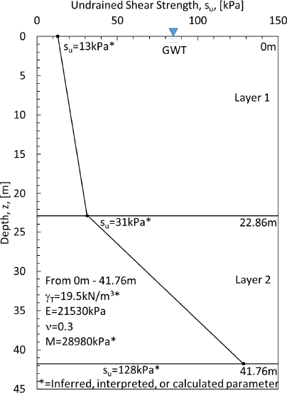
***Figure E1. Soil stratigraphy for the Briaud and Tucker (1997) Example Problem 1 design example (modified to include additional required design parameters).***

Table E1. Briaud and Tucker (1997) Example Problem 1 PILENEG Program input data.

Pile Material	Concrete
Pile Shape	Octagonal
Pile Face [mm]	174*
Pile Perimeter [m]	1.39
Pile Area [m²]	0.145
Pile Embedded Length [m]	41.76
Pile Modulus [kN/m²]	2.41 x 10⁷
Top Load on Pile [kN]	2225
Number of Pile Increments	50
Soil Young’s Modulus [kN/m²]	21531
Soil Poisson’s Ratio	0.3
Soil Ultimate Bearing Capacity [kN/m²]	7097
Ground Water Table Depth [m]	0*
* Inferred or interpolated parameters using correlations contained in Briaud and Tucker (1997).

Page 117

Suggested Citation: "Appendix E: Design Example 3 - Embankment Fill Over Clay (SHANSEP) Using Hand Calculations." National Academies of Sciences, Engineering, and Medicine. 2024. Pile Design for Downdrag: Examples and Supporting Materials. Washington, DC: The National Academies Press. doi: 10.17226/27864.

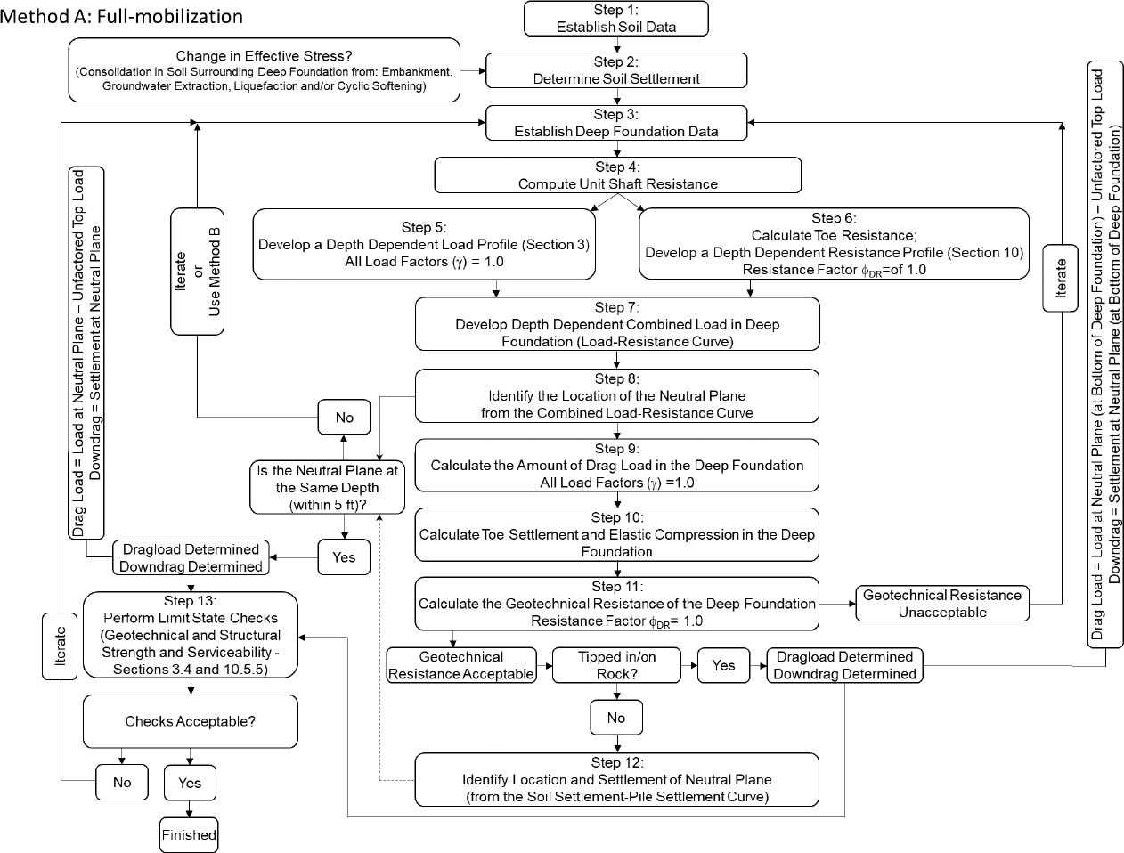
mobilization) procedures proposed by the NCHRP12-116A project team. The flowchart proposed by the NCHRP12-116A was followed.

Step 1: Establish soil data

The pile parameters that were required were obtained from Briaud and Tucker (1997). These parameters are listed in Table E1. As with Design Example 1, the soil modulus (M) presented in Figure E1 was calculated using Equation 1 based on the Young’s modulus (E) and Poisson’s ratio (ν) values for the soil as provided in Briaud and Tucker (1997). The initial pre-consolidation undrained shear strength values were determined by converting the provided Briaud and Tucker (1997) friction data to undrained shear strength data (Figure E2).

Page 118

Suggested Citation: "Appendix E: Design Example 3 - Embankment Fill Over Clay (SHANSEP) Using Hand Calculations." National Academies of Sciences, Engineering, and Medicine. 2024. Pile Design for Downdrag: Examples and Supporting Materials. Washington, DC: The National Academies Press. doi: 10.17226/27864.

presentation

Page 119

Suggested Citation: "Appendix E: Design Example 3 - Embankment Fill Over Clay (SHANSEP) Using Hand Calculations." National Academies of Sciences, Engineering, and Medicine. 2024. Pile Design for Downdrag: Examples and Supporting Materials. Washington, DC: The National Academies Press. doi: 10.17226/27864.

M = \frac{E (1 - v)}{(1 + v) (1 - 2 v)}

Eqn. 1

Step 2: Determine soil settlement

The soil profile shown in Figure E1 was discretized into sublayers (50 sublayers, each 0.835m thick) and then the effective stress at the center of each sublayer was calculated using a submerged unit weight of 9.69 kN/m³ below the ground water table for the two-layer clay soil profile. The effective stress (σ_z′) was determined using Terzaghi’s effective stress equation with the ground water table assumed to be at the original ground surface as shown previously in Figure E1. The settlement profile shown in Figure E3 was created by using the aforementioned sublayers and then calculating the amount of settlement within each sublayer resulting from a 6m thick, 8m crest, 32m base embankment fill, with a unit weight of 19.5kN/m³, being placed on top of the two-layer clay soil profile (Figure E4).

Figure E2. Relationship between maximum friction and undrained shear strength (modified from Briaud and Tucker, 1997). Undrained shear strength values used as the initial pre-consolidation undrained shear strength for this design example (Design Example 3).

The settlement profile presented in Figure E3 was developed for points below the center of the embankment using the Osterberg embankment stress distribution which used a symmetric geometry and provided half of the actual stress influence (Figure E4 and Equations 2 through 4).

I = \frac{1}{π} [(\frac{B_{1} + B_{2}}{B_{2}}) (α_{1} + α_{2}) - \frac{B_{1}}{B_{2}} (α_{1})]

Eqn. 2

α_{1} (r a d i a n s) = t a n^{- 1} (\frac{B_{1}}{z})

Eqn. 3

α_{2} (r a d i a n s) = t a n^{- 1} (\frac{B_{1} + B_{2}}{z}) - t a n^{- 1} (\frac{B_{1}}{z})

Eqn. 4

For the geometry shown in Figure E4, the embankment was symmetric about the central axis, and the amount of settlement (δ) was determined at different depths along this line of symmetry. Therefore, the influence factor (I), as computed using Equation 2 was multiplied by two (2) to account for

Figure E3. Calculated soil settlement profile for an embankment fill (Fig. 4) placed on the soil profile presented previously in Figure E1.

Page 120

Suggested Citation: "Appendix E: Design Example 3 - Embankment Fill Over Clay (SHANSEP) Using Hand Calculations." National Academies of Sciences, Engineering, and Medicine. 2024. Pile Design for Downdrag: Examples and Supporting Materials. Washington, DC: The National Academies Press. doi: 10.17226/27864.

both halves of the embankment about the line of symmetry. The increase in stress (∆σ) at each sublayer depth (z) was then calculated as the product of the influence factor and the bearing pressure (q=γ_fillH_fill=117kPa) resulting from the embankment. The α₁ and α₂ parameters from Figure E4, along with the Σ(I), ∆σ, and δ values that were calculated for each sublayer are included as Table E2. The consolidation strain (ε_z) presented in Table E2 was calculated by dividing the change in stress (∆σ) by the constrained modulus (M). The vertical settlement was determined as the product of the consolidation strain and the sublayer thickness.

***Figure E4. Schematic of the embankment evaluated using the Osterberg embankment stress distributions.***

SHANSEP Analysis

A SHANSEP analysis was performed to determine the amount of increase in the shear strength of the soil resulting from consolidation of the soil being subjected to the embankment loading. A modified form of the SHANSEP equation is presented as Equation 5. The S and m parameters found in Equation 5 are curve-fitting parameters. Minimum values of S (0.14) and m (0.7) were selected for use. The initial undrained shear strength (s_u,o) profile as a function of depth, as shown previously in Figure E1, and the initial vertical effective stress ( $\bar{σ_{z, o}} = σ_{z, o}^{'}$ ) from Table E2 were used to determine the $\frac{s_{u, o}}{σ_{z, 0}}$ ratio prior to placement of the embankment load. Equation 5 was rearranged to determine the over-consolidation ratio prior to placement of the embankment (OCR_{pre−embankment}) as shown in Equation 6. As calculated in Equation 7, the post-embankment vertical effective stress ( $\bar{σ_{z, f}} = σ_{z, f}^{'}$ ) within each sublayer was equal to the sum of the initial vertical effective stress ( $\bar{σ_{z, o}} = σ_{z, o}^{'}$ ) and the change in stress within each sublayer that was shown in Table E2. The pre-embankment over-consolidation ratio was then used to determine the maximum past pressure (Equation 8). As calculated in Equation 8, the maximum past pressure ( $\bar{σ_{m a x}} = σ_{m a x}^{'}$ ) was taken as the maximum value of the post-embankment vertical effective stress ( $\bar{σ_{z, f}} = σ_{z, f}^{'}$ ) or the calculated maximum past pressure that was determined as the product of the OCR_{pre−embankment} and the pre-embankment vertical effective stress. Minimum values of S (0.14) and m (0.7) were also used in Equation 10 to determine the $\frac{s_{u, f}}{σ_{z, f}}$ ratio. Using Equation 11, the $\frac{s_{u, f}}{σ_{z, f}}$ ratio was then used with the final vertical effective stress ( $\bar{σ_{z, f}}$ ) to determine the resultant final undrained shear strength (s_u_,f). The results of the calculations performed using Equations 5 through 11 are contained in Table E3. The initial undrained shear strength and final undrained shear strength are compared in Figure E5.

Page 121

Suggested Citation: "Appendix E: Design Example 3 - Embankment Fill Over Clay (SHANSEP) Using Hand Calculations." National Academies of Sciences, Engineering, and Medicine. 2024. Pile Design for Downdrag: Examples and Supporting Materials. Washington, DC: The National Academies Press. doi: 10.17226/27864.

Table E2. Calculated soil settlement parameters.

Layer Depth [m]			z [m]	Thickness [m]	σ_z,o′ [kPa]	α₁ [rad]	α₂ [rad]	Σ(I)	∆σ [kPa]	ε_z	δ [m]
0	-	0.8352	0.4176	0.8352	4.0465	1.4668	0.0779	0.9999	116.9912	0.0040	0.0034
0.8352	-	1.6704	1.2528	0.8352	12.1396	1.2673	0.2254	0.9981	116.7756	0.0040	0.0034
1.6704	-	2.5056	2.088	0.8352	20.2327	1.0897	0.3513	0.9919	116.0572	0.0040	0.0033
2.5056	-	3.3408	2.9232	0.8352	28.3258	0.9397	0.4504	0.9805	114.7226	0.0040	0.0033
3.3408	-	4.176	3.7584	0.8352	36.4189	0.8165	0.5236	0.9642	112.8139	0.0039	0.0033
4.176	-	5.0112	4.5936	0.8352	44.5120	0.7164	0.5748	0.9440	110.4464	0.0038	0.0032
5.0112	-	5.8464	5.4288	0.8352	52.6051	0.6350	0.6087	0.9209	107.7477	0.0037	0.0031
5.8464	-	6.6816	6.264	0.8352	60.6982	0.5683	0.6293	0.8960	104.8309	0.0036	0.0030
6.6816	-	7.5168	7.0992	0.8352	68.7912	0.5131	0.6401	0.8700	101.7873	0.0035	0.0029
7.5168	-	8.352	7.9344	0.8352	76.8843	0.4669	0.6435	0.8435	98.6867	0.0034	0.0028
8.352	-	9.1872	8.7696	0.8352	84.9774	0.4279	0.6415	0.8169	95.5815	0.0033	0.0028
9.1872	-	10.0224	9.6048	0.8352	93.0705	0.3946	0.6355	0.7907	92.5100	0.0032	0.0027
10.0224	-	10.8576	10.44	0.8352	101.1636	0.3659	0.6268	0.7650	89.4999	0.0031	0.0026
10.8576	-	11.6928	11.2752	0.8352	109.2567	0.3409	0.6160	0.7399	86.5704	0.0030	0.0025
11.6928	-	12.528	12.1104	0.8352	117.3498	0.3190	0.6039	0.7157	83.7345	0.0029	0.0024
12.528	-	13.3632	12.9456	0.8352	125.4429	0.2997	0.5909	0.6923	81.0005	0.0028	0.0023
13.3632	-	14.1984	13.7808	0.8352	133.5360	0.2825	0.5773	0.6699	78.3730	0.0027	0.0023
14.1984	-	15.0336	14.616	0.8352	141.6290	0.2671	0.5634	0.6483	75.8540	0.0026	0.0022
15.0336	-	15.8688	15.4512	0.8352	149.7221	0.2533	0.5495	0.6277	73.4433	0.0025	0.0021
15.8688	-	16.704	16.2864	0.8352	157.8152	0.2408	0.5357	0.6080	71.1395	0.0025	0.0021
16.704	-	17.5392	17.1216	0.8352	165.9083	0.2295	0.5220	0.5892	68.9400	0.0024	0.0020
17.5392	-	18.3744	17.9568	0.8352	174.0014	0.2192	0.5087	0.5713	66.8415	0.0023	0.0019
18.3744	-	19.2096	18.792	0.8352	182.0945	0.2097	0.4956	0.5542	64.8402	0.0022	0.0019
19.2096	-	20.0448	19.6272	0.8352	190.1876	0.2010	0.4829	0.5379	62.9321	0.0022	0.0018
20.0448	-	20.88	20.4624	0.8352	198.2807	0.1930	0.4706	0.5223	61.1129	0.0021	0.0018
20.88	-	21.7152	21.2976	0.8352	206.3737	0.1857	0.4587	0.5075	59.3784	0.0020	0.0017
21.7152	-	22.5504	22.1328	0.8352	214.4668	0.1788	0.4471	0.4934	57.7242	0.0020	0.0017
22.5504	-	23.3856	22.968	0.8352	222.5599	0.1724	0.4360	0.4799	56.1463	0.0019	0.0016
23.3856	-	24.2208	23.8032	0.8352	230.6530	0.1665	0.4253	0.4670	54.6405	0.0019	0.0016
24.2208	-	25.056	24.6384	0.8352	238.7461	0.1609	0.4150	0.4547	53.2030	0.0018	0.0015
25.056	-	25.8912	25.4736	0.8352	246.8392	0.1558	0.4051	0.4430	51.8301	0.0018	0.0015
25.8912	-	26.7264	26.3088	0.8352	254.9323	0.1509	0.3955	0.4318	50.5182	0.0017	0.0015
26.7264	-	27.5616	27.144	0.8352	263.0254	0.1463	0.3863	0.4211	49.2638	0.0017	0.0014
27.5616	-	28.3968	27.9792	0.8352	271.1184	0.1420	0.3775	0.4108	48.0640	0.0017	0.0014
28.3968	-	29.232	28.8144	0.8352	279.2115	0.1379	0.3689	0.4010	46.9155	0.0016	0.0014
29.232	-	30.0672	29.6496	0.8352	287.3046	0.1341	0.3608	0.3916	45.8156	0.0016	0.0013
30.0672	-	30.9024	30.4848	0.8352	295.3977	0.1305	0.3529	0.3826	44.7616	0.0015	0.0013
30.9024	-	31.7376	31.32	0.8352	303.4908	0.1270	0.3453	0.3739	43.7510	0.0015	0.0013
31.7376	-	32.5728	32.1552	0.8352	311.5839	0.1238	0.3380	0.3657	42.7814	0.0015	0.0012
32.5728	-	33.408	32.9904	0.8352	319.6770	0.1207	0.3309	0.3577	41.8506	0.0014	0.0012
33.408	-	34.2432	33.8256	0.8352	327.7701	0.1177	0.3241	0.3501	40.9566	0.0014	0.0012
34.2432	-	35.0784	34.6608	0.8352	335.8632	0.1149	0.3176	0.3427	40.0973	0.0014	0.0012
35.0784	-	35.9136	35.496	0.8352	343.9562	0.1122	0.3113	0.3356	39.2710	0.0014	0.0011
35.9136	-	36.7488	36.3312	0.8352	352.0493	0.1097	0.3052	0.3289	38.4759	0.0013	0.0011
36.7488	-	37.584	37.1664	0.8352	360.1424	0.1072	0.2993	0.3223	37.7104	0.0013	0.0011
37.584	-	38.4192	38.0016	0.8352	368.2355	0.1049	0.2936	0.3160	36.9730	0.0013	0.0011
38.4192	-	39.2544	38.8368	0.8352	376.3286	0.1026	0.2882	0.3099	36.2624	0.0013	0.0010
39.2544	-	40.0896	39.672	0.8352	384.4217	0.1005	0.2829	0.3041	35.5770	0.0012	0.0010
40.0896	-	40.9248	40.5072	0.8352	392.5148	0.0984	0.2778	0.2984	34.9158	0.0012	0.0010
40.9248	-	41.76	41.3424	0.8352	400.6079	0.0965	0.2728	0.2930	34.2774	0.0012	0.0010
z = layer midpoint depth, _z,o′ = vertical effective stress, ₁ and ₂ = angles (in radians) as shown in Figure E4, _z = vertical consolidation strain, = vertical settlement of individual sublayer; (from bottom to top) = settlement profile (Figure E3).

Page 122

Suggested Citation: "Appendix E: Design Example 3 - Embankment Fill Over Clay (SHANSEP) Using Hand Calculations." National Academies of Sciences, Engineering, and Medicine. 2024. Pile Design for Downdrag: Examples and Supporting Materials. Washington, DC: The National Academies Press. doi: 10.17226/27864.

\frac{S_{u, o}}{σ_{z, o}} = S * {(O C R_{p r e - e m b a n k m e n t})}^{m}

Eqn. 5

(\frac{\frac{S_{u, o}}{σ_{z, o}}}{S}) = O C R_{p r e - e m b a n k m e n t}

Eqn. 6

\bar{σ_{z, f}} = \bar{σ_{z, o}} + Δ σ

Eqn. 7

\bar{σ_{m a x}} = m a x {\begin{matrix} O C R_{p r e - e m b a n k m e n t} \cdot \bar{σ_{z, o}} \\ \bar{σ_{z, f}} \end{matrix}}

Eqn. 8

O C R_{p r e - e m b a n k m e n t} = \bar{σ_{m a x}} \cdot \bar{σ_{z, f}}

Eqn. 9

\frac{S_{u, f}}{σ_{z, f}} = S - {(O C R_{p r e - e m b a n k m e n t})}^{m}

Eqn. 10

S_{u, f} = (\frac{s_{u, f}}{σ_{z, f}} \cdot \bar{σ_{z, f}})

Eqn. 11

***Figure E5. Pre- and post-embankment undrained shear strength profiles.***

The final undrained shear strength values that were obtained from the SHANSEP analysis were then used to determine the unit side resistance acting along the pile. Like Design Example 1, the unit side shear was determined by using the total stress analysis “α method”. Specifically, the procedure and equations (Equations 12 and 13) recommended in Randolph and Murphy (1985) were used.

For $s_{u, f} / σ_{z, f} \leq 1$ :

α = \frac{{(\frac{s_{u}}{σ_{s 0}^{'}})}_{N C}^{0.5}}{{(\frac{s_{u, f}}{σ_{z, f}^{'}})}^{0.5}}

Eqn. 12

For $s_{u, f} / σ_{z, f} > 1$ :

α = \frac{{(\frac{s_{u}}{σ_{s 0}^{'}})}_{N C}^{0.5}}{{(\frac{s_{u, f}}{σ_{z, f}^{'}})}^{0.25}}

Eqn. 13

with ${(\frac{s_{u}}{σ_{z, 0}^{'}})}_{N C} = 0.22$

Step 3: Establish pile data

The pile data required to determine the drag load and downdrag include 1) the unit side resistance acting on the pile(s), 2) the end bearing resistance provided by the pile(s), 3) the unfactored pile head deadload, and 3) the elastic compression of the pile(s). Multiple pile types or pile geometries may be considered to determine the magnitude of downdrag/drag load on the pile(s). To compute the drag load for a given design scenario, the following pile data is required: pile material, pile diameter or pile perimeter, pile cross-sectional area, and pile modulus. The pile considered for this design example was an octagonal pile; the pile diameter was therefore not required. The pile material (pre-stressed concrete), perimeter (1.39m), cross-sectional area (0.145m²), and pile modulus (2.41x107 kN/m²) were considered in this example.

Page 123

Suggested Citation: "Appendix E: Design Example 3 - Embankment Fill Over Clay (SHANSEP) Using Hand Calculations." National Academies of Sciences, Engineering, and Medicine. 2024. Pile Design for Downdrag: Examples and Supporting Materials. Washington, DC: The National Academies Press. doi: 10.17226/27864.

Step 4: Compute incremental side resistance

The nominal unit side resistance (f_n) for each sublayer was calculated by multiplying the calculated α factor by the final post-consolidation undrained shear strength using Equation 14. Likewise, the side resistance (F_s) for each sublayer was determined by multiplying the nominal side resistance by the area of the pile in contact with the soil within the given sublayer (Equation 15). The total side resistance for the pile was determined by summing the side resistance from each sublayer. The calculated values for each sublayer, including the final vertical effective stress (σ_z,f′), final undrained shear strength (s_u,f), alpha value (α), nominal unit side resistance (f_n), and side resistance (F_s) are presented in Table E4.

f_{n} = α (s_{u, f})

Eqn. 14

F_{s} = f_{n} A_{s}

Eqn. 15

Steps 5 and 6: Develop the depth-dependent load profile, compute end bearing and a depth-dependent resistance profile

The load and resistance profile graphs were developed by determining the cumulative load in the pile, as a function of depth, from the top of the pile to the bottom of the pile for the load curve and from the bottom of the pile to the top of the pile for the resistance curve. The unfactored top load (2225 kN) was added to the cumulative load in the pile for the load curve. The end bearing resistance, as calculated using Equations 16 and 17, was added to the cumulative load in the pile for the resistance curve. For the clay profile that was investigated, the end bearing resistance (Rt) was calculated using the final undrained shear strength at the toe of the pile (s_u,f) and the cross-sectional area at the end of the pile (A_t). The values of load and resistance for each sublayer are included in Table E5. Also included in Table E5 are the segmental elastic compression and cumulative elastic compression (as measured from the bottom to the pile to the top of the pile). The elastic compression was calculated using Equations 17 and 18.

q_{n}^{'} = 9 \cdot s_{u, f}

Eqn. 16

R_{t} = q_{n}^{'} \cdot A_{t}

Eqn. 17

δ_{E C, s} = \frac{(M i n [\begin{matrix} Q \\ R \end{matrix}]) L_{s}}{A E}

Eqn. 18

δ_{E C} = Σ (δ_{E C, s}) | from toe of pile to top of pile

Eqn. 19

Page 124

Suggested Citation: "Appendix E: Design Example 3 - Embankment Fill Over Clay (SHANSEP) Using Hand Calculations." National Academies of Sciences, Engineering, and Medicine. 2024. Pile Design for Downdrag: Examples and Supporting Materials. Washington, DC: The National Academies Press. doi: 10.17226/27864.

Table E3. SHANSEP calculated parameters.

Layer Depth [m]			σ_z,o′ [kPa]	s_u,o [kPa]	s_u,o/σ_z,o′	OCR_pre	σ_z,f′ [kPa]	σ′_max [kPa]	OCR_post	s_u,f/σ_z,f′	s_u,f [kPa]
0	-	0.8352	4.0465	13.2882	3.2838	90.6788	121.0378	366.9358	3.0316	0.3043	36.8313
0.8352	-	1.6704	12.1396	13.9549	1.1495	20.2430	128.9152	245.7423	1.9062	0.2199	28.3501
1.6704	-	2.5056	20.2327	14.6215	0.7227	10.4304	136.2899	211.0351	1.5484	0.1901	25.9129
2.5056	-	3.3408	28.3258	15.2882	0.5397	6.8740	143.0484	194.7108	1.3612	0.1737	24.8511
3.3408	-	4.176	36.4189	15.9548	0.4381	5.1023	149.2328	185.8210	1.2452	0.1632	24.3587
4.176	-	5.0112	44.5120	16.6215	0.3734	4.0613	154.9584	180.7763	1.1666	0.1559	24.1653
5.0112	-	5.8464	52.6051	17.2882	0.3286	3.3839	160.3528	178.0108	1.1101	0.1506	24.1526
5.8464	-	6.6816	60.6982	17.9548	0.2958	2.9115	165.5291	176.7201	1.0676	0.1466	24.2600
6.6816	-	7.5168	68.7912	18.6215	0.2707	2.5649	170.5785	176.4447	1.0344	0.1434	24.4530
7.5168	-	8.352	76.8843	19.2881	0.2509	2.3009	175.5710	176.9007	1.0076	0.1407	24.7101
8.352	-	9.1872	84.9774	19.9548	0.2348	2.0935	180.5589	180.5589	1.0000	0.1400	25.2782
9.1872	-	10.0224	93.0705	20.6214	0.2216	1.9268	185.5806	185.5806	1.0000	0.1400	25.9813
10.0224	-	10.8576	101.1636	21.2881	0.2104	1.7899	190.6635	190.6635	1.0000	0.1400	26.6929
10.8576	-	11.6928	109.2567	21.9548	0.2009	1.6758	195.8271	195.8271	1.0000	0.1400	27.4158
11.6928	-	12.528	117.3498	22.6214	0.1928	1.5792	201.0843	201.0843	1.0000	0.1400	28.1518
12.528	-	13.3632	125.4429	23.2881	0.1856	1.4965	206.4434	206.4434	1.0000	0.1400	28.9021
13.3632	-	14.1984	133.5360	23.9547	0.1794	1.4250	211.9090	211.9090	1.0000	0.1400	29.6673
14.1984	-	15.0336	141.6290	24.6214	0.1738	1.3625	217.4830	217.4830	1.0000	0.1400	30.4476
15.0336	-	15.8688	149.7221	25.2881	0.1689	1.3075	223.1655	223.1655	1.0000	0.1400	31.2432
15.8688	-	16.704	157.8152	25.9547	0.1645	1.2587	228.9547	228.9547	1.0000	0.1400	32.0537
16.704	-	17.5392	165.9083	26.6214	0.1605	1.2151	234.8483	234.8483	1.0000	0.1400	32.8788
17.5392	-	18.3744	174.0014	27.2880	0.1568	1.1760	240.8429	240.8429	1.0000	0.1400	33.7180
18.3744	-	19.2096	182.0945	27.9547	0.1535	1.1407	246.9347	246.9347	1.0000	0.1400	34.5709
19.2096	-	20.0448	190.1876	28.6213	0.1505	1.1087	253.1197	253.1197	1.0000	0.1400	35.4368
20.0448	-	20.88	198.2807	29.2880	0.1477	1.0796	259.3936	259.3936	1.0000	0.1400	36.3151
20.88	-	21.7152	206.3737	29.9547	0.1451	1.0529	265.7521	265.7521	1.0000	0.1400	37.2053
21.7152	-	22.5504	214.4668	30.6213	0.1428	1.0285	272.1910	272.1910	1.0000	0.1400	38.1067
22.5504	-	23.3856	222.5599	31.7574	0.1427	1.0276	278.7062	278.7062	1.0000	0.1400	39.0189
23.3856	-	24.2208	230.6530	36.0542	0.1563	1.1705	285.2935	285.2935	1.0000	0.1400	39.9411
24.2208	-	25.056	238.7461	40.3510	0.1690	1.3087	291.9491	312.4493	1.0702	0.1468	42.8614
25.056	-	25.8912	246.8392	44.6478	0.1809	1.4419	298.6693	355.9218	1.1917	0.1583	47.2752
25.8912	-	26.7264	254.9323	48.9447	0.1920	1.5701	305.4504	400.2735	1.3104	0.1692	51.6726
26.7264	-	27.5616	263.0254	53.2415	0.2024	1.6934	312.2892	445.3964	1.4262	0.1795	56.0554
27.5616	-	28.3968	271.1184	57.5383	0.2122	1.8118	319.1824	491.2005	1.5389	0.1893	60.4256
28.3968	-	29.232	279.2115	61.8351	0.2215	1.9255	326.1270	537.6098	1.6485	0.1986	64.7845
29.232	-	30.0672	287.3046	66.1319	0.2302	2.0346	333.1202	584.5598	1.7548	0.2075	69.1335
30.0672	-	30.9024	295.3977	70.4287	0.2384	2.1395	340.1593	631.9952	1.8579	0.2160	73.4738
30.9024	-	31.7376	303.4908	74.7255	0.2462	2.2402	347.2418	679.8683	1.9579	0.2241	77.8063
31.7376	-	32.5728	311.5839	79.0224	0.2536	2.3369	354.3653	728.1376	2.0548	0.2318	82.1321
32.5728	-	33.408	319.6770	83.3192	0.2606	2.4298	361.5276	776.7668	2.1486	0.2391	86.4518
33.408	-	34.2432	327.7701	87.6160	0.2673	2.5192	368.7267	825.7242	2.2394	0.2462	90.7661
34.2432	-	35.0784	335.8632	91.9128	0.2737	2.6052	375.9605	874.9815	2.3273	0.2529	95.0758
35.0784	-	35.9136	343.9562	96.2096	0.2797	2.6879	383.2272	924.5140	2.4124	0.2593	99.3812
35.9136	-	36.7488	352.0493	100.5064	0.2855	2.7675	390.5252	974.2995	2.4948	0.2655	103.6830
36.7488	-	37.584	360.1424	104.8032	0.2910	2.8442	397.8528	1024.3180	2.5746	0.2714	107.9814
37.584	-	38.4192	368.2355	109.1000	0.2963	2.9181	405.2085	1074.5520	2.6518	0.2771	112.2770
38.4192	-	39.2544	376.3286	113.3969	0.3013	2.9894	412.5909	1124.9855	2.7266	0.2825	116.5700
39.2544	-	40.0896	384.4217	117.6937	0.3062	3.0581	419.9987	1175.6040	2.7991	0.2878	120.8607
40.0896	-	40.9248	392.5148	121.9905	0.3108	3.1245	427.4305	1226.3945	2.8692	0.2928	125.1494
40.9248	-	41.76	400.6079	126.2873	0.3152	3.1885	434.8853	1277.3453	2.9372	0.2976	129.4364
_z,o′ = initial vertical effective stress, s_u,o=initial undrained shear strength, s_u,o/_z,o′=initial c/p ratio, OCR_pre= pre-embankment over-consolidation ratio, _z,f′ = final vertical effective stress, ′max=maximum past pressure, OCR_post= post-embankment over-consolidation ratio, s_u,f/_z,f′= final c/p ratio, s_u,f=final undrained shear strength

Page 125

Suggested Citation: "Appendix E: Design Example 3 - Embankment Fill Over Clay (SHANSEP) Using Hand Calculations." National Academies of Sciences, Engineering, and Medicine. 2024. Pile Design for Downdrag: Examples and Supporting Materials. Washington, DC: The National Academies Press. doi: 10.17226/27864.

Table E4. Calculated pile side resistance parameters.

Layer Depth [m]			z [m]	Thickness [m]	σ_z,f′ [kPa]	s_u,f [kPa]	α	f_n [kPa]	F_s [kN]
0	-	0.8352	0.4176	0.8352	121.0378	36.83	0.85	0.00	0.00
0.8352	-	1.6704	1.2528	0.8352	128.9152	28.35	1.00	28.36	32.92
1.6704	-	2.5056	2.088	0.8352	136.2899	25.91	1.08	27.87	32.36
2.5056	-	3.3408	2.9232	0.8352	143.0484	24.85	1.13	27.97	32.47
3.3408	-	4.176	3.7584	0.8352	149.2328	24.36	1.16	28.28	32.83
4.176	-	5.0112	4.5936	0.8352	154.9584	24.17	1.19	28.70	33.32
5.0112	-	5.8464	5.4288	0.8352	160.3528	24.15	1.21	29.19	33.89
5.8464	-	6.6816	6.264	0.8352	165.5291	24.26	1.23	29.72	34.51
6.6816	-	7.5168	7.0992	0.8352	170.5785	24.45	1.24	30.29	35.17
7.5168	-	8.352	7.9344	0.8352	175.5710	24.71	1.25	30.89	35.87
8.352	-	9.1872	8.7696	0.8352	180.5589	25.28	1.25	31.69	36.79
9.1872	-	10.0224	9.6048	0.8352	185.5806	25.98	1.25	32.57	37.81
10.0224	-	10.8576	10.44	0.8352	190.6635	26.69	1.25	33.46	38.85
10.8576	-	11.6928	11.2752	0.8352	195.8271	27.42	1.25	34.37	39.90
11.6928	-	12.528	12.1104	0.8352	201.0843	28.15	1.25	35.29	40.97
12.528	-	13.3632	12.9456	0.8352	206.4434	28.90	1.25	36.23	42.06
13.3632	-	14.1984	13.7808	0.8352	211.9090	29.67	1.25	37.19	43.17
14.1984	-	15.0336	14.616	0.8352	217.4830	30.45	1.25	38.17	44.31
15.0336	-	15.8688	15.4512	0.8352	223.1655	31.24	1.25	39.17	45.47
15.8688	-	16.704	16.2864	0.8352	228.9547	32.05	1.25	40.18	46.65
16.704	-	17.5392	17.1216	0.8352	234.8483	32.88	1.25	41.22	47.85
17.5392	-	18.3744	17.9568	0.8352	240.8429	33.72	1.25	42.27	49.07
18.3744	-	19.2096	18.792	0.8352	246.9347	34.57	1.25	43.34	50.31
19.2096	-	20.0448	19.6272	0.8352	253.1197	35.44	1.25	44.42	51.57
20.0448	-	20.88	20.4624	0.8352	259.3936	36.32	1.25	45.52	52.85
20.88	-	21.7152	21.2976	0.8352	265.7521	37.21	1.25	46.64	54.14
21.7152	-	22.5504	22.1328	0.8352	272.1910	38.11	1.25	47.77	55.46
22.5504	-	23.3856	22.968	0.8352	278.7062	39.02	1.25	48.91	56.78
23.3856	-	24.2208	23.8032	0.8352	285.2935	39.94	1.25	50.07	58.13
24.2208	-	25.056	24.6384	0.8352	291.9491	42.86	1.22	52.47	60.91
25.056	-	25.8912	25.4736	0.8352	298.6693	47.28	1.18	55.73	64.70
25.8912	-	26.7264	26.3088	0.8352	305.4504	51.67	1.14	58.93	68.41
26.7264	-	27.5616	27.144	0.8352	312.2892	56.06	1.11	62.06	72.05
27.5616	-	28.3968	27.9792	0.8352	319.1824	60.43	1.08	65.14	75.62
28.3968	-	29.232	28.8144	0.8352	326.1270	64.78	1.05	68.18	79.15
29.232	-	30.0672	29.6496	0.8352	333.1202	69.13	1.03	71.18	82.63
30.0672	-	30.9024	30.4848	0.8352	340.1593	73.47	1.01	74.15	86.08
30.9024	-	31.7376	31.32	0.8352	347.2418	77.81	0.99	77.10	89.50
31.7376	-	32.5728	32.1552	0.8352	354.3653	82.13	0.97	80.02	92.90
32.5728	-	33.408	32.9904	0.8352	361.5276	86.45	0.96	82.92	96.27
33.408	-	34.2432	33.8256	0.8352	368.7267	90.77	0.95	85.81	99.62
34.2432	-	35.0784	34.6608	0.8352	375.9605	95.08	0.93	88.68	102.95
35.0784	-	35.9136	35.496	0.8352	383.2272	99.38	0.92	91.54	106.27
35.9136	-	36.7488	36.3312	0.8352	390.5252	103.68	0.91	94.38	109.57
36.7488	-	37.584	37.1664	0.8352	397.8528	107.98	0.90	97.22	112.86
37.584	-	38.4192	38.0016	0.8352	405.2085	112.28	0.89	100.05	116.15
38.4192	-	39.2544	38.8368	0.8352	412.5909	116.57	0.88	102.86	119.42
39.2544	-	40.0896	39.672	0.8352	419.9987	120.86	0.87	105.68	122.68
40.0896	-	40.9248	40.5072	0.8352	427.4305	125.15	0.87	108.48	125.94
40.9248	-	41.76	41.3424	0.8352	434.8853	129.44	0.86	111.28	129.19
z = layer midpoint depth, _z,f′ = vertical effective stress, s_u,f = undrained shear strength, = total stress side resistance parameter, f_n=nominal unit side resistance, F_s=sublayer side resistance. Note: f_n neglected for top 1.5m

Page 126

Suggested Citation: "Appendix E: Design Example 3 - Embankment Fill Over Clay (SHANSEP) Using Hand Calculations." National Academies of Sciences, Engineering, and Medicine. 2024. Pile Design for Downdrag: Examples and Supporting Materials. Washington, DC: The National Academies Press. doi: 10.17226/27864.

Steps 7 through 12: Develop a depth-dependent combined load profile for the pile (Step 7) to: identify the location of the neutral plane (Step 8), calculate the amount of drag load (Step 9), calculate the toe settlement and elastic compression (Step 10), calculate the geotechnical resistance (Step 11), and identify the locations of the neutral plane from the soil settlement-pile settlement curve (Step 12)

A combined load and resistance curve, comprised of the minimum value of load or resistance for each sublayer, is presented in Figure E6a. Also included in Figure E6a, and used for comparison, is the combined load-resistance curve that was developed in Design Example 1. The soil settlement-pile settlement curve is presented in Figure E6b; this curve was developed using the elastic compression values presented in Table E5. The tip movement obtained using the DeCock (2009) method based on Chin’s Hyperbolic Model in Step 11 of Design Example 1 was also reused for this design example.

The neutral plane location that was determined from the combined load and resistance curve (14.20m) was different than the neutral plane location that was identified with the soil settlement-pile settlement curve (11.27m). Although a difference in the location of the neutral plane should not be observed when evaluating based on the combined load and resistance curve or based on the soil settlement-pile settlement curve, a difference was also observed for the case presented in Design Example 1. In Design Example 1, the neutral plane location that was determined from the combined load and resistance curve was 13.36m while the neutral plane location that was identified with the soil settlement-pile settlement curve was 12.11m. Therefore, the calculated depths for the location of the neutral plane in Design Example 3 were lower and higher than the corresponding depths that were obtained when not accounting for strength gain as obtained from the combined load and resistance curve or based on the soil settlement-pile settlement curve, respectively.

The amount of calculated drag load in the pile almost doubled (from 286kN in Design Example 1 to 582kN in Design Example 3) due to the strength gain associated with consolidation of the soil surrounding the pile. Although the drag load almost doubled, the depth of the neutral plane, as predicted using the combined load-settlement curve, did not change significantly (the location of the neutral plane moved downward by approximately 0.5m between Design Example 1 and Design Example 3 when evaluating based on the combined load and resistance curve). The amount of settlement at the neutral plane (downdrag) was 0.0576m. This calculated downdrag was slightly greater than the 0.0550m that was calculated for Design Example 1. The increased shear strength in the soil surrounding the pile and the additional amount of pile compression were observed to contribute to the increase in calculated drag load.

When comparing the locations of the neutral plane obtained during Step 8 (14.20m) and Step 12 (11.27m), the neutral plane locations were not within the required 5ft (1.5m). The additional elastic compression in the pile resulting from the increase in drag load in the pile caused the location of the neutral plane to move up from (12.11m in Design Example 1 to 11.27m in Design Example 3). Because the locations of the neutral planes obtained from Steps 8 and 12 were greater than 5ft (1.5m), the geometry of the pile should be changed (length increased or diameter increased) and the design process iterated (Step 3 through Step 12).

Page 127

Suggested Citation: "Appendix E: Design Example 3 - Embankment Fill Over Clay (SHANSEP) Using Hand Calculations." National Academies of Sciences, Engineering, and Medicine. 2024. Pile Design for Downdrag: Examples and Supporting Materials. Washington, DC: The National Academies Press. doi: 10.17226/27864.

Table E5. Calculated load as a function of depth.

Layer Depth			z	Q	R	$M i n [\begin{matrix} Q \\ R \end{matrix}]$	δ_EC,s	δ_EC	Comments: z=depth, Q=load, R=resistance, δ_EC,s=segmental elastic compression, δ_EC=cumulative elastic compression (from bottom to top), A=pile cross-sectional area=0.145[m²] E_p=pile elastic modulus=2.41E+07[kPa] L_s=length of each pile segment=0.8532[m]
[m]			[m]	[kN]	[kN]	[kN]	[m]	[m]
0	-	0.8352	0.4176	2225.00	3377.24	2225.00	0.0005	0.0242
0.8352	-	1.6704	1.2528	2257.92	3377.24	2257.92	0.0005	0.0236
1.6704	-	2.5056	2.088	2290.28	3344.32	2290.28	0.0005	0.0231
2.5056	-	3.3408	2.9232	2322.74	3311.96	2322.74	0.0006	0.0226
3.3408	-	4.176	3.7584	2355.58	3279.50	2355.58	0.0006	0.0220
4.176	-	5.0112	4.5936	2388.90	3246.67	2388.90	0.0006	0.0214
5.0112	-	5.8464	5.4288	2422.78	3213.35	2422.78	0.0006	0.0209
5.8464	-	6.6816	6.264	2457.29	3179.46	2457.29	0.0006	0.0203
6.6816	-	7.5168	7.0992	2492.46	3144.95	2492.46	0.0006	0.0197
7.5168	-	8.352	7.9344	2528.32	3109.79	2528.32	0.0006	0.0191
8.352	-	9.1872	8.7696	2565.11	3073.92	2565.11	0.0006	0.0185
9.1872	-	10.0224	9.6048	2602.92	3037.13	2602.92	0.0006	0.0179
10.0224	-	10.8576	10.44	2641.77	2999.32	2641.77	0.0006	0.0173
10.8576	-	11.6928	11.2752	2681.67	2960.48	2681.67	0.0006	0.0166
11.6928	-	12.528	12.1104	2722.64	2920.58	2722.64	0.0007	0.0160
12.528	-	13.3632	12.9456	2764.70	2879.61	2764.70	0.0007	0.0153
13.3632	-	14.1984	13.7808	2807.87	2837.55	2807.87	0.0007	0.0147
14.1984	-	15.0336	14.616	2852.18	2794.37	2794.37	0.0007	0.0140
15.0336	-	15.8688	15.4512	2897.65	2750.06	2750.06	0.0007	0.0133
15.8688	-	16.704	16.2864	2944.30	2704.59	2704.59	0.0006	0.0127
16.704	-	17.5392	17.1216	2992.15	2657.95	2657.95	0.0006	0.0120
17.5392	-	18.3744	17.9568	3041.22	2610.10	2610.10	0.0006	0.0114
18.3744	-	19.2096	18.792	3091.53	2561.03	2561.03	0.0006	0.0108
19.2096	-	20.0448	19.6272	3143.10	2510.72	2510.72	0.0006	0.0102
20.0448	-	20.88	20.4624	3195.95	2459.15	2459.15	0.0006	0.0096
20.88	-	21.7152	21.2976	3250.09	2406.30	2406.30	0.0006	0.0090
21.7152	-	22.5504	22.1328	3305.55	2352.15	2352.15	0.0006	0.0084
22.5504	-	23.3856	22.968	3362.33	2296.69	2296.69	0.0005	0.0078
23.3856	-	24.2208	23.8032	3420.46	2239.91	2239.91	0.0005	0.0073
24.2208	-	25.056	24.6384	3481.37	2181.78	2181.78	0.0005	0.0068
25.056	-	25.8912	25.4736	3546.08	2120.87	2120.87	0.0005	0.0062
25.8912	-	26.7264	26.3088	3614.48	2056.17	2056.17	0.0005	0.0057
26.7264	-	27.5616	27.144	3686.53	1987.76	1987.76	0.0005	0.0052
27.5616	-	28.3968	27.9792	3762.15	1915.71	1915.71	0.0005	0.0048
28.3968	-	29.232	28.8144	3841.30	1840.09	1840.09	0.0004	0.0043
29.232	-	30.0672	29.6496	3923.94	1760.94	1760.94	0.0004	0.0039
30.0672	-	30.9024	30.4848	4010.02	1678.31	1678.31	0.0004	0.0035
30.9024	-	31.7376	31.32	4099.52	1592.22	1592.22	0.0004	0.0030
31.7376	-	32.5728	32.1552	4192.42	1502.72	1502.72	0.0004	0.0027
32.5728	-	33.408	32.9904	4288.69	1409.82	1409.82	0.0003	0.0023
33.408	-	34.2432	33.8256	4388.30	1313.56	1313.56	0.0003	0.0020
34.2432	-	35.0784	34.6608	4491.25	1213.94	1213.94	0.0003	0.0017
35.0784	-	35.9136	35.496	4597.52	1110.99	1110.99	0.0003	0.0014
35.9136	-	36.7488	36.3312	4707.09	1004.73	1004.73	0.0002	0.0011
36.7488	-	37.584	37.1664	4819.95	895.15	895.15	0.0002	0.0009
37.584	-	38.4192	38.0016	4936.10	782.29	782.29	0.0002	0.0006
38.4192	-	39.2544	38.8368	5055.51	666.15	666.15	0.0002	0.0005
39.2544	-	40.0896	39.672	5178.20	546.73	546.73	0.0001	0.0003
40.0896	-	40.9248	40.5072	5304.14	424.05	424.05	0.0001	0.0002
40.9248	-	41.76	41.3424	5433.33	298.11	298.11	0.0001	0.0001

Page 128

Suggested Citation: "Appendix E: Design Example 3 - Embankment Fill Over Clay (SHANSEP) Using Hand Calculations." National Academies of Sciences, Engineering, and Medicine. 2024. Pile Design for Downdrag: Examples and Supporting Materials. Washington, DC: The National Academies Press. doi: 10.17226/27864.

***Figure E6. a) Combined load-settlement curves with and without accounting for soil strength gain, and b) soil settlement-pile settlement curve.***

Step 13: Perform limit state checks

The comparisons of the locations of the neutral planes obtained from Step 8 and Step 12 yielded unsatisfactory results and the design process should have been iterated prior to proceeding with step 13. However, for the sake of brevity, limit state checks were performed to determine if the pile size was suitable for the design loads. For the structural strength limit state, the determined drag load (582kN) was multiplied by the drag load factor (γ_DR=1.1) to obtain a factored load of drag load 640kN. The unfactored top load (2225kN) placed on the top of the pile was multiplied by the deadload factor (γ_D=1.25) to obtain a factored deadload of 2781kN. The combined total factored load was 3422kN. The concrete compressive strength for the pre-stressed concrete pile was assumed to be 5000psi (34474kPa) resulting in a factored structural stress of 25856kPa (0.75*34474kPa) and a factored structural strength of 3749kN when the stress was multiplied by the cross-sectional area of the pile (0.145m²). If a concrete compressive strength of 5000psi (34474kPa), was used for the pre-stressed pile then the pile is adequately sized because the factored structural strength (3749kN) was determined to be greater than the combined total factored load (3096kN). If a lower-strength concrete was used for the pre-stressed concrete pile, then the pile would need to be larger in cross-sectional area or lengthened. Either modification to the pile would result in a change in the amount of drag load on the pile; Steps 3 through 13 of the NCHRP12-116A flowchart would need to be repeated to ensure the factored structural strength was greater than the total factored load.

Page 129

Suggested Citation: "Appendix E: Design Example 3 - Embankment Fill Over Clay (SHANSEP) Using Hand Calculations." National Academies of Sciences, Engineering, and Medicine. 2024. Pile Design for Downdrag: Examples and Supporting Materials. Washington, DC: The National Academies Press. doi: 10.17226/27864.

Conclusion:

The SHANSEP method was used in this design example to determine the influence of an increase in shear strength of the soil, resulting from reconsolidation, on the downdrag and drag load within a pile foundation. In this analysis, both the drag load and the downdrag were observed to increase. This increase in drag load resulted in a change in the location of the neutral plane when obtained from the soil settlement-pile settlement curve. The geometry of the pile should have been modified to ensure the locations of the neutral plane that were obtained in Steps 8 and 12 were within 5ft (1.5m). Although the drag load increased and the locations of the neutral planes were not within 5ft (1.5m), the factored structural strength calculated in Step 13 was sufficient to support the total factored load.

References:

Briaud, J.L., and Tucker, L. (1997). NCHRP Report 393: Design and Construction Guidelines for Downdrag on Uncoated and Bitumen-Coated Piles. TRB, National Research Council, Washington, DC.

Coffman, R.A., Bowders, J.J., and Burton, P.M. (2010). “Use of SHANSEP Design Parameters in Landfill Design: A Cost/Benefit Case Study.” ASCE Geotechnical Special Publication No. 199, Proc. GeoFlorida 2010: Advances in Analysis, Modeling and Design, West Palm Beach, Florida. 2859–2866.

DeCock, F.A. (2009). “Sense and Sensitivity of Pile Load-Deformation Behavior.” Deep Foundation on Board and Auger Piles. Taylor and Francis. 22 pp.

Ladd, C.C., and Foott, R., (1974) “New Design Procedure for Stability of Soft Clays,” Journal of Geotechnical Engineering Division, Vol. 100, No. GT7, July.

Ladd, C.C., and D.J. DeGroot. (2003). “Recommended Practice for Soft Ground Characterization.” Proceedings of Soil and Rock America 2003, 12th Pan-American Conference on Soil Mechanics and Geotechnical Engineering and 39th U.S. Rock Mechanics Symposium 1: 3–57

Loehr, J.E., Lutenegger, A., Rosenblad, B., and Bowckmann, A. (2016). Geotechnical Site Characterization Geotechnical Engineering Circular No. 5. Report No. FHWA NHI-16-072. Washington, DC. 688 pp.

Randolph, M.F., Murphy, B.S. (1985). “Shaft Capacity of Driven Piles in Clay.” Proceedings of the 1985 Offshore Technology Conference. Paper No. OTC-4883-MS. May 6-9. Houston, TX.

Stuedlein, A.W., Saye, S.R., and Kumm, B.P. (2020). “SHANSEP-Based Side Resistance of Driven Pipe Piles in Plastic Soils: Revision and LRFD Calibration.” Journal of Geotechnical and Geoenvironmental Engineering 146 (8): 06020010.