Pile Design for Downdrag: Examples and Supporting Materials (2024)
Chapter: Appendix F: Design Example 4 - Drawdown in Clay Using TZPILE
APPENDIX F
Design Example 4 — Drawdown in Clay Using TZPILE
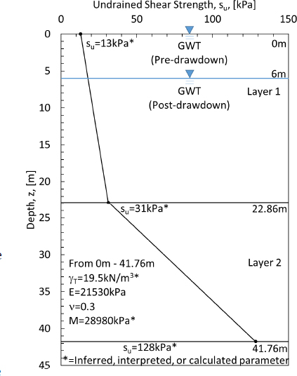
Design Example Problem 4, contained herein, uses the same design data that was presented in Design Example 1. Like Design Example 1, the design data were acquired from Briaud and Tucker (1997). The focus of Design Example 1 was on determining the amount of drag load and downdrag resulting from an embankment being placed at the ground surface. The focus of Design Example 4 is on determining the amount of drag load and downdrag resulting from ground settlement associated with ground water withdrawal. Specifically, as shown in Figure F1, the ground water was assumed to retreat from the ground surface to a depth of 6 meters below the ground surface. As with Design Example 1, the input parameters from the Briaud and Tucker (1997) Example Problem 1 are used for Example 4 and are included in Table F1 for completeness. Procedures for determining the location of the neutral plane and magnitudes of the drag load and downdrag are demonstrated using 1) Load-Resistance profiles and 2) Pile-Soil Settlement profiles by means of the proposed Method B (partial
Table F1. Briaud and Tucker (1997) Example Problem 1 input data.
| Pile Material | Concrete | |
| Pile Shape | Octagonal | |
| Pile Face [mm] | 174* | |
| Pile Perimeter [m] | 1.39 | |
| Pile Area [m2] | 0.145 | |
| Pile Embedded Length [m] | 41.76 | |
| Pile Modulus [kN/m2] | 2.41 x 10⁷ | |
| Top Load on Pile [kN] | 2225 | |
| Number of Pile Increments | 50 | |
| Maximum Shaft Resistance | Depth [m] | Shaft Resistance [kN/m2] |
| 0 | 12.92, 13*(su B&T Fig. 2.5) | |
| 22.86 | 30.80, 31*(su B&T Fig. 2.5) | |
| 41.76 | 94.18, 128* (su Fig. 2.5) | |
| Soil Young’s Modulus [kN/m2] | 21531 | |
| Soil Poisson’s Ratio | 0.3 | |
| Soil Ultimate Bearing Capacity [kN/m2] | 7097 | |
| Initial Ground Water Table Depth [m] | 0* | |
| * Inferred or interpolated parameters using correlations contained in Briaud and Tucker (1997). Fig. 2.5 in this table refers to Fig. 2.5 from Briaud and Tucker (1997). | ||
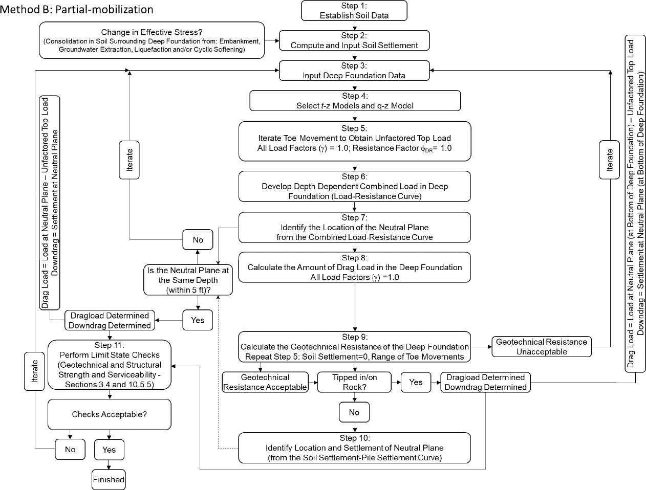
mobilization) procedures proposed by the NCHRP 12-116A project team. The steps of the flowchart developed by the project team were followed. The flowchart is included on the next page.
Step 1: Establish soil data
The soil data for this design example are shown in Figure F1. Additional required soil data including the Young’s modulus and Poissons’ ratio of the soil are presented in Table F1.
The soil profile was discretized into sublayers (50 sublayers, each 0.835m thick). The effective stress at the center of each sublayer was calculated using a total unit weight of 19.5kN/m3 above the ground water table and a submerged unit weight of 9.69kN/m3 below the ground water table for the two-layer clay soil profile.
Step 2: Determine soil settlement
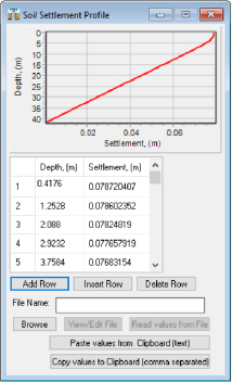
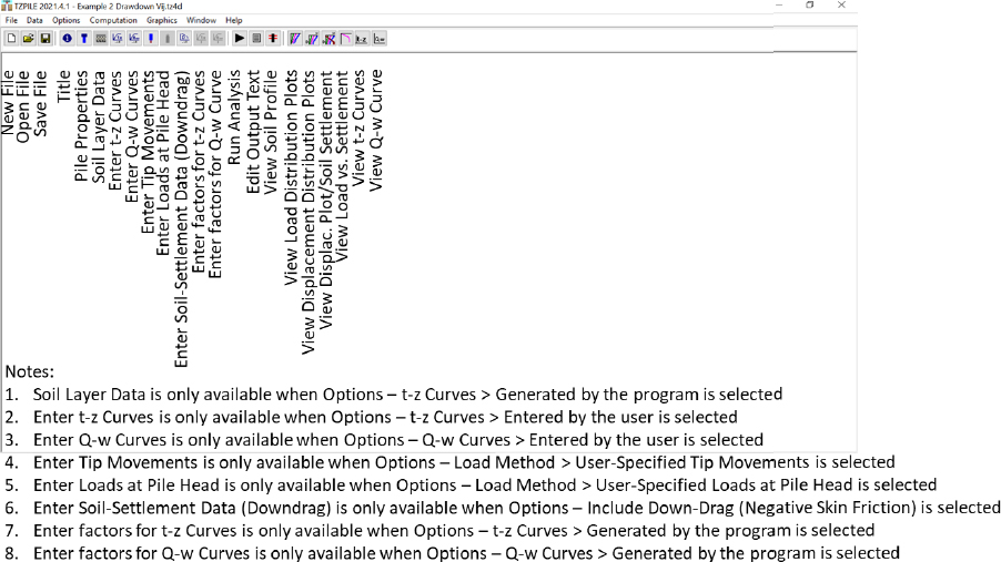
The soil settlement in Design Example 4 was caused by an increase in the effective stress in the soil due to lowering of the ground water instead of an increase in the effective stress in the soil due to an embankment being placed on the ground surface that was presented in Design Example 1. The amount of soil settlement, as a function of depth, is presented in Table F2. The settlement was calculated by first determining the effective stress and then the change in stress for each depth increment (Equation 1). The corresponding amount of strain (εz) for each depth increment was obtained by dividing the change in stress (∆σ) by the constrained modulus (M) of the soil, as shown in Equation 2. The incremental settlement (δincrement) was determined using Equation 3. The cumulative settlement was obtained by accumulating the incremental settlement for each layer from the bottom of the pile to the top of the pile (Equation 4). The calculations used to obtain the cumulative settlement are included in Table F2. The Soil Settlement Profile input window (within the Ensoft TZPILE program) is shown in Figure F2, as selected from the TZPILE ribbon that is shown in Figure F3. Soil Settlement data were entered through the Data - Enter Soil Settlement Data (for Downdrag) selection in the Data drop-down menu (Figure F3). This option is only available for selection if the Options - Include Down-Drag (negative Skin Friction) choice is chosen in the Options tab.
| Eqn. 1 |
| Eqn. 2 |
| Eqn. 3 |
| Eqn. 4 |
Step 3: Establish pile data
The pile data required to determine the drag load and downdrag include 1) the unit side resistance acting on the pile(s), 2) the end bearing resistance provided by the pile(s), and 3) the unfactored pile head deadload. Multiple pile types or pile geometries may be considered to determine the magnitude of downdrag/drag load on the pile(s). To compute the drag load for a given design scenario, the following pile data is required: pile material, pile diameter or pile perimeter, pile cross-sectional area, and pile modulus. The pile material (pre-stressed concrete), perimeter (1.39m), cross-sectional area (0.145m2), and pile modulus (2.41x10⁷ kN/m2) were considered in this example.
Table F2. Calculated soil settlements resulting from drawdown event.
| Layer Depth | z | Thickness | σzo′ | σzf′ | ∆σ | εz | δincrement | Σδreversed | ||
| [m] | [m] | [m] | [kPa] | [kPa] | [kPa] | [m] | [m] | |||
| 0 | - | 0.8352 | 0.4176 | 0.8352 | 8.1432 | 8.1432 | 4.0967 | 0.0001 | 0.0001 | 0.0787 |
| 0.8352 | - | 1.6704 | 1.2528 | 0.8352 | 24.4296 | 24.4296 | 12.2900 | 0.0004 | 0.0004 | 0.0786 |
| 1.6704 | - | 2.5056 | 2.088 | 0.8352 | 40.7160 | 40.7160 | 20.4833 | 0.0007 | 0.0006 | 0.0782 |
| 2.5056 | - | 3.3408 | 2.9232 | 0.8352 | 57.0024 | 57.0024 | 28.6766 | 0.0010 | 0.0008 | 0.0777 |
| 3.3408 | - | 4.176 | 3.7584 | 0.8352 | 73.2888 | 73.2888 | 36.8699 | 0.0013 | 0.0011 | 0.0768 |
| 4.176 | - | 5.0112 | 4.5936 | 0.8352 | 89.5752 | 89.5752 | 45.0632 | 0.0016 | 0.0013 | 0.0758 |
| 5.0112 | - | 5.8464 | 5.4288 | 0.8352 | 105.8616 | 105.8616 | 53.2565 | 0.0018 | 0.0015 | 0.0745 |
| 5.8464 | - | 6.6816 | 6.264 | 0.8352 | 119.5582 | 119.5582 | 58.8600 | 0.0020 | 0.0017 | 0.0729 |
| 6.6816 | - | 7.5168 | 7.0992 | 0.8352 | 127.6512 | 127.6512 | 58.8600 | 0.0020 | 0.0017 | 0.0712 |
| 7.5168 | - | 8.352 | 7.9344 | 0.8352 | 135.7443 | 135.7443 | 58.8600 | 0.0020 | 0.0017 | 0.0695 |
| 8.352 | - | 9.1872 | 8.7696 | 0.8352 | 143.8374 | 143.8374 | 58.8600 | 0.0020 | 0.0017 | 0.0678 |
| 9.1872 | - | 10.0224 | 9.6048 | 0.8352 | 151.9305 | 151.9305 | 58.8600 | 0.0020 | 0.0017 | 0.0662 |
| 10.0224 | - | 10.8576 | 10.44 | 0.8352 | 160.0236 | 160.0236 | 58.8600 | 0.0020 | 0.0017 | 0.0645 |
| 10.8576 | - | 11.6928 | 11.2752 | 0.8352 | 168.1167 | 168.1167 | 58.8600 | 0.0020 | 0.0017 | 0.0628 |
| 11.6928 | - | 12.528 | 12.1104 | 0.8352 | 176.2098 | 176.2098 | 58.8600 | 0.0020 | 0.0017 | 0.0611 |
| 12.528 | - | 13.3632 | 12.9456 | 0.8352 | 184.3029 | 184.3029 | 58.8600 | 0.0020 | 0.0017 | 0.0594 |
| 13.3632 | - | 14.1984 | 13.7808 | 0.8352 | 192.3960 | 192.3960 | 58.8600 | 0.0020 | 0.0017 | 0.0577 |
| 14.1984 | - | 15.0336 | 14.616 | 0.8352 | 200.4890 | 200.4890 | 58.8600 | 0.0020 | 0.0017 | 0.0560 |
| 15.0336 | - | 15.8688 | 15.4512 | 0.8352 | 208.5821 | 208.5821 | 58.8600 | 0.0020 | 0.0017 | 0.0543 |
| 15.8688 | - | 16.704 | 16.2864 | 0.8352 | 216.6752 | 216.6752 | 58.8600 | 0.0020 | 0.0017 | 0.0526 |
| 16.704 | - | 17.5392 | 17.1216 | 0.8352 | 224.7683 | 224.7683 | 58.8600 | 0.0020 | 0.0017 | 0.0509 |
| 17.5392 | - | 18.3744 | 17.9568 | 0.8352 | 232.8614 | 232.8614 | 58.8600 | 0.0020 | 0.0017 | 0.0492 |
| 18.3744 | - | 19.2096 | 18.792 | 0.8352 | 240.9545 | 240.9545 | 58.8600 | 0.0020 | 0.0017 | 0.0475 |
| 19.2096 | - | 20.0448 | 19.6272 | 0.8352 | 249.0476 | 249.0476 | 58.8600 | 0.0020 | 0.0017 | 0.0458 |
| 20.0448 | - | 20.88 | 20.4624 | 0.8352 | 257.1407 | 257.1407 | 58.8600 | 0.0020 | 0.0017 | 0.0441 |
| 20.88 | - | 21.7152 | 21.2976 | 0.8352 | 265.2337 | 265.2337 | 58.8600 | 0.0020 | 0.0017 | 0.0424 |
| 21.7152 | - | 22.5504 | 22.1328 | 0.8352 | 273.3268 | 273.3268 | 58.8600 | 0.0020 | 0.0017 | 0.0407 |
| 22.5504 | - | 23.3856 | 22.968 | 0.8352 | 281.4199 | 281.4199 | 58.8600 | 0.0020 | 0.0017 | 0.0390 |
| 23.3856 | - | 24.2208 | 23.8032 | 0.8352 | 289.5130 | 289.5130 | 58.8600 | 0.0020 | 0.0017 | 0.0373 |
| 24.2208 | - | 25.056 | 24.6384 | 0.8352 | 297.6061 | 297.6061 | 58.8600 | 0.0020 | 0.0017 | 0.0356 |
| 25.056 | - | 25.8912 | 25.4736 | 0.8352 | 305.6992 | 305.6992 | 58.8600 | 0.0020 | 0.0017 | 0.0339 |
| 25.8912 | - | 26.7264 | 26.3088 | 0.8352 | 313.7923 | 313.7923 | 58.8600 | 0.0020 | 0.0017 | 0.0322 |
| 26.7264 | - | 27.5616 | 27.144 | 0.8352 | 321.8854 | 321.8854 | 58.8600 | 0.0020 | 0.0017 | 0.0305 |
| 27.5616 | - | 28.3968 | 27.9792 | 0.8352 | 329.9784 | 329.9784 | 58.8600 | 0.0020 | 0.0017 | 0.0288 |
| 28.3968 | - | 29.232 | 28.8144 | 0.8352 | 338.0715 | 338.0715 | 58.8600 | 0.0020 | 0.0017 | 0.0271 |
| 29.232 | - | 30.0672 | 29.6496 | 0.8352 | 346.1646 | 346.1646 | 58.8600 | 0.0020 | 0.0017 | 0.0254 |
| 30.0672 | - | 30.9024 | 30.4848 | 0.8352 | 354.2577 | 354.2577 | 58.8600 | 0.0020 | 0.0017 | 0.0237 |
| 30.9024 | - | 31.7376 | 31.32 | 0.8352 | 362.3508 | 362.3508 | 58.8600 | 0.0020 | 0.0017 | 0.0221 |
| 31.7376 | - | 32.5728 | 32.1552 | 0.8352 | 370.4439 | 370.4439 | 58.8600 | 0.0020 | 0.0017 | 0.0204 |
| 32.5728 | - | 33.408 | 32.9904 | 0.8352 | 378.5370 | 378.5370 | 58.8600 | 0.0020 | 0.0017 | 0.0187 |
| 33.408 | - | 34.2432 | 33.8256 | 0.8352 | 386.6301 | 386.6301 | 58.8600 | 0.0020 | 0.0017 | 0.0170 |
| 34.2432 | - | 35.0784 | 34.6608 | 0.8352 | 394.7232 | 394.7232 | 58.8600 | 0.0020 | 0.0017 | 0.0153 |
| 35.0784 | - | 35.9136 | 35.496 | 0.8352 | 402.8162 | 402.8162 | 58.8600 | 0.0020 | 0.0017 | 0.0136 |
| 35.9136 | - | 36.7488 | 36.3312 | 0.8352 | 410.9093 | 410.9093 | 58.8600 | 0.0020 | 0.0017 | 0.0119 |
| 36.7488 | - | 37.584 | 37.1664 | 0.8352 | 419.0024 | 419.0024 | 58.8600 | 0.0020 | 0.0017 | 0.0102 |
| 37.584 | - | 38.4192 | 38.0016 | 0.8352 | 427.0955 | 427.0955 | 58.8600 | 0.0020 | 0.0017 | 0.0085 |
| 38.4192 | - | 39.2544 | 38.8368 | 0.8352 | 435.1886 | 435.1886 | 58.8600 | 0.0020 | 0.0017 | 0.0068 |
| 39.2544 | - | 40.0896 | 39.672 | 0.8352 | 443.2817 | 443.2817 | 58.8600 | 0.0020 | 0.0017 | 0.0051 |
| 40.0896 | - | 40.9248 | 40.5072 | 0.8352 | 451.3748 | 451.3748 | 58.8600 | 0.0020 | 0.0017 | 0.0034 |
| 40.9248 | - | 41.76 | 41.3424 | 0.8352 | 459.4679 | 459.4679 | 58.8600 | 0.0020 | 0.0017 | 0.0017 |
| z = layer midpoint depth, σzo′ = vertical effective stress, σzf′ = final effective stress, ∆σ = change in effective stress, εz = incremental soil strain, δincrement = incremental soil settlement, Σδreversed = soil settlement from tip of pile to top of pile. | ||||||||||
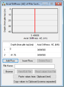
All of the parameters that are required for determination of the neutral plane location were input into the TZPILE program (Ensoft, 2021) by means of several drop-down windows. For example, the pile length, pile head coordinate, number of increments, outer diameter, and area of pile tip, are input through the pop-out window selected using Data – Pile Properties (Figure F4). The additional tab of Edit AE vs. Depth tab within the Data – Pile Properties window must be selected for an additional window to appear to input the axial stiffness, AE, the product of the cross-sectional area, and the Young’s modulus of the pile (Figure F5).

Step 4: Select the t-z models and the q-z model
Within the Ensoft (2021) TZPILE program, mobilized soil resistance can be input into the program through two mechanisms. Specifically, t-z curves and q-z (termed Q-w in TZPILE) curves can either be 1) generated by the program or 2) entered by the user. The procedures to develop the required load curves using either the generated by the program method or the entered by the user method are described herein.
Generated by the program
If t-z curves are “Generated by the program” under the Options – t-z Curves > Generated by the program setting, then the soil stratigraphy shown from Figure F1 can be directly input into the TZPILE program using the Data – Soil Layers pop-out window and sub-windows (Figure F6). Using the drop-down tabs pop-out windows within the Data – Soil Layers pop-out window, the soil type/t-z model of each layer is selected, the bottom depth of the layer for each layer is indicated, and the layer data for each layer is input. Available t-z models within the “Generated by the program” option include: “Driven Pile in Clay (Coyle and Reese)”, “Driven Pile in Sand (Mosher)”, “Drilled Shaft in Clay (Reese and O’Neill)”, “Drilled Shaft in Sand (Reese and O’Neill)”, “Driven Pile in Clay (API)”, “Driven Pile in Sand (API)”. Values are input by selecting the layer data tab for each individual layer to bring up the layer data pop-out window for each layer. The input values of e50 were selected based on the recommended values (ranging from 0.005 to 0.02) for the given clay layer, as found in the Ensoft (2021) TZPILE Technical Manual. The input values of Ultimate Unit Side Friction and Ultimate Unit Tip Resistance were calculated using a spreadsheet similar to the spreadsheet created for Example Problem 1.
The specified inputs (Figure F6) included the soil type and properties above the ground water table in Layer 1, the soil type and properties below the ground water table in Layer 1, the soil type and properties below the ground water table in Layer 2, and a continuation/extrapolation of the parameters used at the bottom of Layer 2 to a depth of 100 m.
The Ultimate Unit Side Friction [kN/m2] values that are input into the layer data windows in the TZPILE software (Figure F6) were determined by using the total stress analysis “α method” because the undrained shear strength (su) parameters were provided. This procedure used to calculate these values was similar to the procedure provided in Step 4 of Example Problem 1. Specifically, the procedure and equations (Equations 1 and 2) recommended in Randolph and Murphy (1985) were used to determine an alpha (α) value for each depth. The effective stress (σz0′) used in Equations 5 or 6 was determined using Terzaghi’s effective stress equation with the ground water table assumed to be at the ground surface for the pre-drawdown condition. The effective stress was calculated at the center of each sublayer.
For :
| Eqn. 5 |
For :
| Eqn. 6 |
with

The nominal unit side resistance (fn) for each sublayer was then calculated by multiplying the α factor by the undrained shear strength using Equation 7. Likewise, the side resistance (Fs) for each sublayer was determined by multiplying the nominal side resistance by the surface area of the pile in contact with the soil within the given sublayer (Equation 8). The total side resistance for the pile was determined by summing the side resistance from each sublayer along the length of the pile.
| Eqn. 7 |
| Eqn. 8 |
The values that were calculated for the pre-drawdown condition, using the aforementioned equations, are included in Table F3, whereas those calculated for the post-drawdown condition are included in Table F4. The values in each table include the vertical effective stress (σvo′), undrained shear strength (su), alpha value (α), nominal side resistance (fn), and side resistance (Fs) obtained for each sublayer. The undrained shear strength values that are presented in Tables F3 and F4 are identical even though strengthening of the soil due to consolidation is expected.
The Ultimate Unit Tip Resistance Values [kN/m2] values that were input into the TZPILE software were determined in a manner that was similar to the procedure provided in Step 6 of Example Problem 1. As shown in Equations 9 and 10, the end bearing resistance (R) was calculated for the top and bottom of each layer using the undrained shear strength (su), as taken from the depth increment of the sublayer that was closest to the depth of the top and the bottom of each layer, respectively. The area at the end of the pile (At) is required for the calculations in the TZPILE software. The Ultimate Unit Tip Resistance [kN/m2] in the TZPILE software was set equivalent to the calculated end bearing resistance (R) that is shown in Table F5. Although an Ultimate Unit Tip Resistance value is included for each layer, the Ultimate Unit Tip Resistance is not required for the layers where only side resistance contributes to the resistance.
Table F3. Calculated pile side resistance parameters for the pre-drawdown condition.
| Layer Depth | z | Thickness | γ | σzo′ | su | α | fn | Fs | ||
| [m] | [m] | [m] | [kN/m3] | [kPa] | [kPa] | [kPa] | [kN] | |||
| 0 | - | 0.8352 | 0.4176 | 0.8352 | 19.5 | 4.0465 | 13.29 | 0.35 | 0.00 | 0.00 |
| 0.8352 | - | 1.6704 | 1.2528 | 0.8352 | 19.5 | 12.1396 | 13.95 | 0.45 | 6.32 | 7.34 |
| 1.6704 | - | 2.5056 | 2.088 | 0.8352 | 19.5 | 20.2327 | 14.62 | 0.55 | 8.07 | 9.37 |
| 2.5056 | - | 3.3408 | 2.9232 | 0.8352 | 19.5 | 28.3258 | 15.29 | 0.64 | 9.76 | 11.33 |
| 3.3408 | - | 4.176 | 3.7584 | 0.8352 | 19.5 | 36.4189 | 15.95 | 0.71 | 11.31 | 13.13 |
| 4.176 | - | 5.0112 | 4.5936 | 0.8352 | 19.5 | 44.5120 | 16.62 | 0.77 | 12.76 | 14.81 |
| 5.0112 | - | 5.8464 | 5.4288 | 0.8352 | 19.5 | 52.6051 | 17.29 | 0.82 | 14.14 | 16.42 |
| 5.8464 | - | 6.6816 | 6.264 | 0.8352 | 19.5 | 60.6982 | 17.95 | 0.86 | 15.48 | 17.98 |
| 6.6816 | - | 7.5168 | 7.0992 | 0.8352 | 19.5 | 68.7912 | 18.62 | 0.90 | 16.79 | 19.49 |
| 7.5168 | - | 8.352 | 7.9344 | 0.8352 | 19.5 | 76.8843 | 19.29 | 0.94 | 18.06 | 20.97 |
| 8.352 | - | 9.1872 | 8.7696 | 0.8352 | 19.5 | 84.9774 | 19.95 | 0.97 | 19.31 | 22.42 |
| 9.1872 | - | 10.0224 | 9.6048 | 0.8352 | 19.5 | 93.0705 | 20.62 | 1.00 | 20.55 | 23.86 |
| 10.0224 | - | 10.8576 | 10.44 | 0.8352 | 19.5 | 101.1636 | 21.29 | 1.02 | 21.77 | 25.27 |
| 10.8576 | - | 11.6928 | 11.2752 | 0.8352 | 19.5 | 109.2567 | 21.95 | 1.05 | 22.97 | 26.67 |
| 11.6928 | - | 12.528 | 12.1104 | 0.8352 | 19.5 | 117.3498 | 22.62 | 1.07 | 24.17 | 28.06 |
| 12.528 | - | 13.3632 | 12.9456 | 0.8352 | 19.5 | 125.4429 | 23.29 | 1.09 | 25.35 | 29.43 |
| 13.3632 | - | 14.1984 | 13.7808 | 0.8352 | 19.5 | 133.5360 | 23.95 | 1.11 | 26.53 | 30.80 |
| 14.1984 | - | 15.0336 | 14.616 | 0.8352 | 19.5 | 141.6290 | 24.62 | 1.12 | 27.70 | 32.16 |
| 15.0336 | - | 15.8688 | 15.4512 | 0.8352 | 19.5 | 149.7221 | 25.29 | 1.14 | 28.86 | 33.51 |
| 15.8688 | - | 16.704 | 16.2864 | 0.8352 | 19.5 | 157.8152 | 25.95 | 1.16 | 30.02 | 34.85 |
| 16.704 | - | 17.5392 | 17.1216 | 0.8352 | 19.5 | 165.9083 | 26.62 | 1.17 | 31.17 | 36.19 |
| 17.5392 | - | 18.3744 | 17.9568 | 0.8352 | 19.5 | 174.0014 | 27.29 | 1.18 | 32.32 | 37.52 |
| 18.3744 | - | 19.2096 | 18.792 | 0.8352 | 19.5 | 182.0945 | 27.95 | 1.20 | 33.46 | 38.85 |
| 19.2096 | - | 20.0448 | 19.6272 | 0.8352 | 19.5 | 190.1876 | 28.62 | 1.21 | 34.61 | 40.17 |
| 20.0448 | - | 20.88 | 20.4624 | 0.8352 | 19.5 | 198.2807 | 29.29 | 1.22 | 35.74 | 41.50 |
| 20.88 | - | 21.7152 | 21.2976 | 0.8352 | 19.5 | 206.3737 | 29.95 | 1.23 | 36.88 | 42.81 |
| 21.7152 | - | 22.5504 | 22.1328 | 0.8352 | 19.5 | 214.4668 | 30.62 | 1.24 | 38.01 | 44.13 |
| 22.5504 | - | 23.3856 | 22.968 | 0.8352 | 19.5 | 222.5599 | 31.76 | 1.24 | 39.43 | 45.78 |
| 23.3856 | - | 24.2208 | 23.8032 | 0.8352 | 19.5 | 230.6530 | 36.05 | 1.19 | 42.77 | 49.66 |
| 24.2208 | - | 25.056 | 24.6384 | 0.8352 | 19.5 | 238.7461 | 40.35 | 1.14 | 46.04 | 53.45 |
| 25.056 | - | 25.8912 | 25.4736 | 0.8352 | 19.5 | 246.8392 | 44.65 | 1.10 | 49.24 | 57.16 |
| 25.8912 | - | 26.7264 | 26.3088 | 0.8352 | 19.5 | 254.9323 | 48.94 | 1.07 | 52.39 | 60.82 |
| 26.7264 | - | 27.5616 | 27.144 | 0.8352 | 19.5 | 263.0254 | 53.24 | 1.04 | 55.51 | 64.44 |
| 27.5616 | - | 28.3968 | 27.9792 | 0.8352 | 19.5 | 271.1184 | 57.54 | 1.02 | 58.58 | 68.01 |
| 28.3968 | - | 29.232 | 28.8144 | 0.8352 | 19.5 | 279.2115 | 61.84 | 1.00 | 61.63 | 71.55 |
| 29.232 | - | 30.0672 | 29.6496 | 0.8352 | 19.5 | 287.3046 | 66.13 | 0.98 | 64.65 | 75.06 |
| 30.0672 | - | 30.9024 | 30.4848 | 0.8352 | 19.5 | 295.3977 | 70.43 | 0.96 | 67.65 | 78.54 |
| 30.9024 | - | 31.7376 | 31.32 | 0.8352 | 19.5 | 303.4908 | 74.73 | 0.95 | 70.63 | 82.00 |
| 31.7376 | - | 32.5728 | 32.1552 | 0.8352 | 19.5 | 311.5839 | 79.02 | 0.93 | 73.60 | 85.44 |
| 32.5728 | - | 33.408 | 32.9904 | 0.8352 | 19.5 | 319.6770 | 83.32 | 0.92 | 76.55 | 88.87 |
| 33.408 | - | 34.2432 | 33.8256 | 0.8352 | 19.5 | 327.7701 | 87.62 | 0.91 | 79.49 | 92.28 |
| 34.2432 | - | 35.0784 | 34.6608 | 0.8352 | 19.5 | 335.8632 | 91.91 | 0.90 | 82.41 | 95.67 |
| 35.0784 | - | 35.9136 | 35.496 | 0.8352 | 19.5 | 343.9562 | 96.21 | 0.89 | 85.32 | 99.06 |
| 35.9136 | - | 36.7488 | 36.3312 | 0.8352 | 19.5 | 352.0493 | 100.51 | 0.88 | 88.23 | 102.43 |
| 36.7488 | - | 37.584 | 37.1664 | 0.8352 | 19.5 | 360.1424 | 104.80 | 0.87 | 91.12 | 105.79 |
| 37.584 | - | 38.4192 | 38.0016 | 0.8352 | 19.5 | 368.2355 | 109.10 | 0.86 | 94.01 | 109.14 |
| 38.4192 | - | 39.2544 | 38.8368 | 0.8352 | 19.5 | 376.3286 | 113.40 | 0.85 | 96.89 | 112.49 |
| 39.2544 | - | 40.0896 | 39.672 | 0.8352 | 19.5 | 384.4217 | 117.69 | 0.85 | 99.77 | 115.82 |
| 40.0896 | - | 40.9248 | 40.5072 | 0.8352 | 19.5 | 392.5148 | 121.99 | 0.84 | 102.64 | 119.15 |
| 40.9248 | - | 41.76 | 41.3424 | 0.8352 | 19.5 | 400.6079 | 126.29 | 0.84 | 105.50 | 122.48 |
| z = layer midpoint depth, σzo′ = vertical effective stress, γ=unit weight, su = undrained shear strength, α = total stress side resistance parameter, fn=nominal unit side resistance, Fs=sublayer side resistance. Note: fn neglected for top 1.5m | ||||||||||
Table F4. Calculated pile side resistance parameters for the post-drawdown condition.
| Layer Depth | z | Thickness | γ | σzo′ | su | α | fn | Fs | ||
| [m] | [m] | [m] | [kN/m3] | [kPa] | [kPa] | [kPa] | [kN] | |||
| 0 | - | 0.8352 | 0.4176 | 0.8352 | 19.5 | 8.1432 | 13.29 | 0.41 | 0.00 | 0.00 |
| 0.8352 | - | 1.6704 | 1.2528 | 0.8352 | 19.5 | 24.4296 | 13.95 | 0.62 | 8.66 | 10.05 |
| 1.6704 | - | 2.5056 | 2.088 | 0.8352 | 19.5 | 40.7160 | 14.62 | 0.78 | 11.44 | 13.29 |
| 2.5056 | - | 3.3408 | 2.9232 | 0.8352 | 19.5 | 57.0024 | 15.29 | 0.91 | 13.85 | 16.07 |
| 3.3408 | - | 4.176 | 3.7584 | 0.8352 | 19.5 | 73.2888 | 15.95 | 1.01 | 16.04 | 18.62 |
| 4.176 | - | 5.0112 | 4.5936 | 0.8352 | 19.5 | 89.5752 | 16.62 | 1.09 | 18.10 | 21.01 |
| 5.0112 | - | 5.8464 | 5.4288 | 0.8352 | 19.5 | 105.8616 | 17.29 | 1.16 | 20.07 | 23.29 |
| 5.8464 | - | 6.6816 | 6.264 | 0.8352 | 19.5 | 119.5582 | 17.95 | 1.21 | 21.73 | 25.23 |
| 6.6816 | - | 7.5168 | 7.0992 | 0.8352 | 19.5 | 127.6512 | 18.62 | 1.23 | 22.87 | 26.55 |
| 7.5168 | - | 8.352 | 7.9344 | 0.8352 | 19.5 | 135.7443 | 19.29 | 1.24 | 24.00 | 27.86 |
| 8.352 | - | 9.1872 | 8.7696 | 0.8352 | 19.5 | 143.8374 | 19.95 | 1.26 | 25.13 | 29.17 |
| 9.1872 | - | 10.0224 | 9.6048 | 0.8352 | 19.5 | 151.9305 | 20.62 | 1.27 | 26.25 | 30.48 |
| 10.0224 | - | 10.8576 | 10.44 | 0.8352 | 19.5 | 160.0236 | 21.29 | 1.29 | 27.38 | 31.78 |
| 10.8576 | - | 11.6928 | 11.2752 | 0.8352 | 19.5 | 168.1167 | 21.95 | 1.30 | 28.50 | 33.08 |
| 11.6928 | - | 12.528 | 12.1104 | 0.8352 | 19.5 | 176.2098 | 22.62 | 1.31 | 29.61 | 34.38 |
| 12.528 | - | 13.3632 | 12.9456 | 0.8352 | 19.5 | 184.3029 | 23.29 | 1.32 | 30.73 | 35.67 |
| 13.3632 | - | 14.1984 | 13.7808 | 0.8352 | 19.5 | 192.3960 | 23.95 | 1.33 | 31.84 | 36.97 |
| 14.1984 | - | 15.0336 | 14.616 | 0.8352 | 19.5 | 200.4890 | 24.62 | 1.34 | 32.95 | 38.26 |
| 15.0336 | - | 15.8688 | 15.4512 | 0.8352 | 19.5 | 208.5821 | 25.29 | 1.35 | 34.06 | 39.55 |
| 15.8688 | - | 16.704 | 16.2864 | 0.8352 | 19.5 | 216.6752 | 25.95 | 1.36 | 35.17 | 40.83 |
| 16.704 | - | 17.5392 | 17.1216 | 0.8352 | 19.5 | 224.7683 | 26.62 | 1.36 | 36.28 | 42.12 |
| 17.5392 | - | 18.3744 | 17.9568 | 0.8352 | 19.5 | 232.8614 | 27.29 | 1.37 | 37.39 | 43.41 |
| 18.3744 | - | 19.2096 | 18.792 | 0.8352 | 19.5 | 240.9545 | 27.95 | 1.38 | 38.50 | 44.69 |
| 19.2096 | - | 20.0448 | 19.6272 | 0.8352 | 19.5 | 249.0476 | 28.62 | 1.38 | 39.60 | 45.97 |
| 20.0448 | - | 20.88 | 20.4624 | 0.8352 | 19.5 | 257.1407 | 29.29 | 1.39 | 40.70 | 47.25 |
| 20.88 | - | 21.7152 | 21.2976 | 0.8352 | 19.5 | 265.2337 | 29.95 | 1.40 | 41.81 | 48.54 |
| 21.7152 | - | 22.5504 | 22.1328 | 0.8352 | 19.5 | 273.3268 | 30.62 | 1.40 | 42.91 | 49.82 |
| 22.5504 | - | 23.3856 | 22.968 | 0.8352 | 19.5 | 281.4199 | 31.76 | 1.40 | 44.34 | 51.48 |
| 23.3856 | - | 24.2208 | 23.8032 | 0.8352 | 19.5 | 289.5130 | 36.05 | 1.33 | 47.92 | 55.63 |
| 24.2208 | - | 25.056 | 24.6384 | 0.8352 | 19.5 | 297.6061 | 40.35 | 1.27 | 51.40 | 59.67 |
| 25.056 | - | 25.8912 | 25.4736 | 0.8352 | 19.5 | 305.6992 | 44.65 | 1.23 | 54.80 | 63.62 |
| 25.8912 | - | 26.7264 | 26.3088 | 0.8352 | 19.5 | 313.7923 | 48.94 | 1.19 | 58.13 | 67.48 |
| 26.7264 | - | 27.5616 | 27.144 | 0.8352 | 19.5 | 321.8854 | 53.24 | 1.15 | 61.40 | 71.28 |
| 27.5616 | - | 28.3968 | 27.9792 | 0.8352 | 19.5 | 329.9784 | 57.54 | 1.12 | 64.63 | 75.03 |
| 28.3968 | - | 29.232 | 28.8144 | 0.8352 | 19.5 | 338.0715 | 61.84 | 1.10 | 67.82 | 78.73 |
| 29.232 | - | 30.0672 | 29.6496 | 0.8352 | 19.5 | 346.1646 | 66.13 | 1.07 | 70.97 | 82.39 |
| 30.0672 | - | 30.9024 | 30.4848 | 0.8352 | 19.5 | 354.2577 | 70.43 | 1.05 | 74.09 | 86.01 |
| 30.9024 | - | 31.7376 | 31.32 | 0.8352 | 19.5 | 362.3508 | 74.73 | 1.03 | 77.18 | 89.60 |
| 31.7376 | - | 32.5728 | 32.1552 | 0.8352 | 19.5 | 370.4439 | 79.02 | 1.02 | 80.25 | 93.17 |
| 32.5728 | - | 33.408 | 32.9904 | 0.8352 | 19.5 | 378.5370 | 83.32 | 1.00 | 83.30 | 96.70 |
| 33.408 | - | 34.2432 | 33.8256 | 0.8352 | 19.5 | 386.6301 | 87.62 | 0.99 | 86.33 | 100.22 |
| 34.2432 | - | 35.0784 | 34.6608 | 0.8352 | 19.5 | 394.7232 | 91.91 | 0.97 | 89.34 | 103.72 |
| 35.0784 | - | 35.9136 | 35.496 | 0.8352 | 19.5 | 402.8162 | 96.21 | 0.96 | 92.34 | 107.20 |
| 35.9136 | - | 36.7488 | 36.3312 | 0.8352 | 19.5 | 410.9093 | 100.51 | 0.95 | 95.32 | 110.66 |
| 36.7488 | - | 37.584 | 37.1664 | 0.8352 | 19.5 | 419.0024 | 104.80 | 0.94 | 98.29 | 114.11 |
| 37.584 | - | 38.4192 | 38.0016 | 0.8352 | 19.5 | 427.0955 | 109.10 | 0.93 | 101.25 | 117.54 |
| 38.4192 | - | 39.2544 | 38.8368 | 0.8352 | 19.5 | 435.1886 | 113.40 | 0.92 | 104.20 | 120.96 |
| 39.2544 | - | 40.0896 | 39.672 | 0.8352 | 19.5 | 443.2817 | 117.69 | 0.91 | 107.13 | 124.37 |
| 40.0896 | - | 40.9248 | 40.5072 | 0.8352 | 19.5 | 451.3748 | 121.99 | 0.90 | 110.06 | 127.78 |
| 40.9248 | - | 41.76 | 41.3424 | 0.8352 | 19.5 | 459.4679 | 126.29 | 0.89 | 112.98 | 131.17 |
| z = layer midpoint depth, σzo′ = vertical effective stress, γ=unit weight, su = undrained shear strength, α = total stress side resistance parameter, fn=nominal unit side resistance, Fs=sublayer side resistance. Note: fn neglected for top 1.5m | ||||||||||
| Eqn. 9 |
| Eqn. 10 |
Table F5. Ultimate Unit Tip Resistance, [kN/m2] values for the four layers used in the TZPILE software.
| TZPILE Depth | Layer Depth | Midpoint Depth | su | At | qn′ | ||
| [m] | [m] | [m] | [kPa] | [m2] | [kPa] | ||
| 0 | 0 | - | 0.8352 | 0.4176 | 13.29 | 0.145 | 119.59 |
| 6 | 5.8464 | - | 6.6816 | 6.264 | 17.95 | 0.145 | 161.59 |
| 22.86 | 21.7152 | - | 22.504 | 22.1328 | 30.62 | 0.145 | 275.59 |
| 41.76 | 40.9248 | - | 41.76 | 41.3424 | 126.29 | 0.145 | 1136.58 |
| 100 | NA | - | NA | NA | NA | NA | NA |
The User-Specified Tip Movements was selected as the Load Method in the Options tab and the Include Down-Drag (negative Skin Friction) option was also selected in the Options drop-down menu. No modification factors were applied to the t-z curves or Q-w curve through the Options drop-down menu.
Entered by the user
If t-z curves are “Entered by the user” under the Options – t-z Curves > Entered by the user setting, then the soil stratigraphy shown previously in Figure F1 cannot be directly input into the TZPILE program. Instead, each layer is represented by a different t-z curve. The t-z curves are input into the TZPILE program by selecting the Data – t-z Curves pop-out window (Figure F7) after previously selecting the Options – t-z Curves > Entered by the user setting. Likewise, a Q-w curve is input for the layer that contains the pile tip by selecting the Data – Q-w curves (Figure F8) after previously selecting the Options – q-w Curve > Entered by the user setting. The t-z and Q-w curves shown in Figures F7 and F8, respectively, were computed using the Vijayvergiya (1977) t-z curve equations (Equations 11 and 12). Key parameters that were used to develop the curves are presented in Table F6.
The settlement limit associated with the side resistance (ss,lim) and the end bearing resistance limit (sb,lim) within the mathematical expressions shown in Equations 11 and 12 are 0.0075m and 0.05B, respectively; with B being the width of the pile at the pile tip. These values were set to 0.0075m and 0.021m for this design example. The fn parameter from the top and bottom of each soil layer, as obtained from Table F2 shown previously, was set equal to the ultimate skin resistance (qs,ult) parameter shown in Equation 11. Likewise, the qn′ value at the pile tip, calculated using Equation 5, was used as the ultimate tip resistance (qb,ult) parameter shown in Equation 12. Ten ss values, ranging from 0.000m to 0.0080m by 0.001m increments were used to develop a t-z curve for each soil layer. Likewise, nine ss values ranging from 0.000m to 0.030m were used to develop the Q-w curve at the pile tip. The values used in the calculations using Equations 11 and 12 are presented in Table F6. The tabulated values for the four t-z curves and one Q-w curve are included in Tables F7 and F8, respectively.


| Eqn. 11 |
| Eqn. 12 |
(from Vijayvergiya, 1977, as reported in Bohn et al., 2017)
Table F6. Design parameters used to develop t-z and Q-w curves.
| Bottom of Layer | |||
| Layer 1a | Depth, z, [m] | 0 | 6 |
| Unit Weight, γ, [kN/m3] | 19.5 | 19.5 | |
| Undrained Shear Strength, su, [kPa] | 12.95 | 17.74 | |
| Ultimate Skin Resistance, fs,ult, [kPa] | 8.66 | 21.73 | |
| Ultimate Tip Resistance, qp,ult, [kPa] | 116.55 | 159.66 | |
| Layer 1b | Depth, z, [m] | 6 | 22.86 |
| Unit Weight, γ, [kN/m3] | 9.69 | 9.69 | |
| Undrained Shear Strength, su, [kPa] | 17.74 | 31.2 | |
| Ultimate Skin Resistance, fs,ult, [kPa] | 21.73 | 42.91 | |
| Ultimate Tip Resistance, qp,ult, [kPa] | 159.66 | 280.8 | |
| Layer 2 | Depth, z, [m] | 22.86 | 41.76 |
| Unit Weight, γ, [kN/m3] | 9.69 | 9.69 | |
| Undrained Shear Strength, su, [kPa] | 31.2 | 128.44 | |
| Ultimate Skin Resistance, fs,ult, [kPa] | 42.91 | 112.98 | |
| Ultimate Tip Resistance, qp,ult, [kPa] | 280.8 | 1155.96 | |
Table F7. Develop t-z curves using Vijayvergiya (1977).
| Displacement, z, [m] (used for all t-z curves) | Layer 1a Top of Layer | Layer 1a Bottom of Layer | Layer 1b Bottom of Layer | Layer 2 Bottom of Layer |
| Load Transfer, t, [kPa] | ||||
| 0.0000 | 0.0000 | 0.0000 | 0.0000 | 0.0000 |
| 0.0010 | 5.1697 | 12.9720 | 25.6157 | 67.4449 |
| 0.0020 | 6.6347 | 16.6480 | 32.8746 | 86.5572 |
| 0.0030 | 7.4901 | 18.7945 | 37.1133 | 97.7177 |
| 0.0040 | 8.0301 | 20.1494 | 39.7887 | 104.7619 |
| 0.0050 | 8.3684 | 20.9983 | 41.4651 | 109.1756 |
| 0.0060 | 8.5635 | 21.4878 | 42.4317 | 111.7208 |
| 0.0070 | 8.6500 | 21.7050 | 42.8607 | 112.8501 |
| 0.0075 | 8.6600 | 21.7300 | 42.9100 | 112.9800 |
| 0.0080 | 8.6507 | 21.7066 | 42.8638 | 112.8585 |
Table F8. Q-w curves using Vijayvergiya (1977).
| Displacement, w, [m] (used for all Q-w curves) | Layer 2 Bottom of Layer Tip Resistance, Q, [kN] |
| 0.0000 | 0.000 |
| 0.0010 | 60.802 |
| 0.0025 | 82.521 |
| 0.0050 | 103.970 |
| 0.0100 | 130.993 |
| 0.0150 | 149.950 |
| 0.0200 | 165.041 |
| 0.0250 | 167.614 |
| 0.0300 | 167.614 |
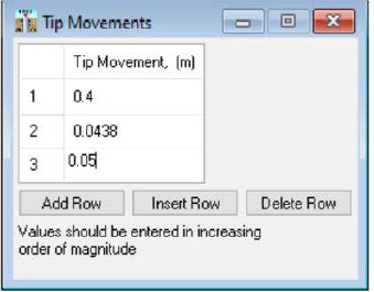

Step 5: Iterate toe movement to obtained unfactored top load
As used previously in Design Example 1 and in the “Generated by the program” section of Design Example 4, the unfactored top load to be placed on the piles is also 2225 kN for the “Entered by the user” section of Design Example 4. During processing in TZPILE, the tip movement was adjusted by selecting Data – Enter Tip Movements within the TZPILE software.
Tip Movements (Figure F9) were entered through the Data – Enter Tip Movements selection in the Data drop-down menu. Likewise, Soil Settlement data was entered through the Data - Enter Soil Settlement Data (for Downdrag) selection in the Data drop-down menu. These options are only available for selection if the Options - Load Method > User-Specified Tip Movement and Options - Include Down-Drag (negative Skin Friction) are chosen in the Options tab. An initial estimate of tip movement (0.0448m) was determined by following the DeCock (2009) solution that was shown in Step 10 of Example Problem 1. The movement was bracketed and iterated until the top load in the pile was equal to the prescribed unfactored load (2225kN) being applied to the pile. An input tip movement of 0.0438m, within the TZPILE program, provided the required 2225kN of top load.
Step 6: Develop the depth-dependent combined load in the pile
After entering the tip movements, the Run Analysis tab in the TZPILE program was selected and the load transfer data was visualized using the View Load Distribution Plots quick link in the ribbon or by selecting Graphics – Load Distribution. The quick links ribbon within the TZPILE software program enabled access to the data. The data can also be exported to Excel for manipulation and/or presentation via the Graphics – Export Plots to Excel popout window (Figure F10). In addition to the combined load-resistance curve, the displacement distribution, soil settlement, axial load vs. settlement, t-z curves (side resistance), and Q-w curve (tip resistance) can also be visualized in the program and/or exported. One Excel file
will be generated with different sheets and charts being created for each of the different Available Plots that were selected.
Step 7: Identify the location of the neutral plane from the combined load-resistance curve
The exported data were plotted in Excel to create the combined load-resistance curve and the soil settlement-pile settlement curve. As shown in Figure F11a, the location of the netural plane was 13.78m. Using the TZPILE program, the locations of the neutral plane that are obtained from the loadresistace curve and from the soil settlement-pile settlement curve will always coexist. The tabulated data that were obtained using the “Entered by user” method in TZPILE are also provided in Table F9.
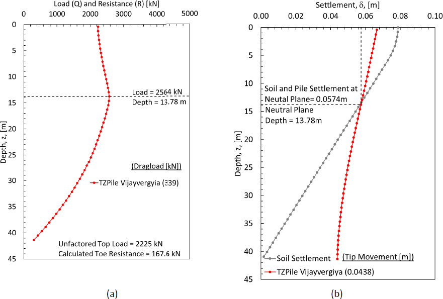
Step 8: Calculate the amount of drag load in the pile
As shown in Figure F11a, the maximum amount of load in the pile occured at the location of the neutral plane (13.78m). The amount of drag load is the maximum load in the pile (2564kN) minus the unfactored top load in the pile (2225kN). Therefore, the drag load was determined to be 339kN.
Table F9. Soil settlement, pile settlement, and combined load and resistance values for Design Example 4.
| z | Combined Load and Resistance | Pile Settlement | Soil Settlement | ||
| V | HC | V | HC | ||
| [m] | [kN] | [m] | [m] | ||
| 41.34 | 306 | 299 | 0.0438 | 0.0449 | 0.0017 |
| 40.51 | 427 | 427 | 0.0439 | 0.0450 | 0.0034 |
| 39.67 | 544 | 551 | 0.0440 | 0.0451 | 0.0051 |
| 38.84 | 658 | 672 | 0.0442 | 0.0453 | 0.0068 |
| 38.00 | 768 | 789 | 0.0444 | 0.0455 | 0.0085 |
| 37.17 | 875 | 904 | 0.0446 | 0.0457 | 0.0102 |
| 36.33 | 979 | 1014 | 0.0448 | 0.0459 | 0.0119 |
| 35.50 | 1079 | 1121 | 0.0450 | 0.0462 | 0.0136 |
| 34.66 | 1176 | 1225 | 0.0453 | 0.0465 | 0.0153 |
| 33.83 | 1270 | 1325 | 0.0456 | 0.0468 | 0.0170 |
| 32.99 | 1360 | 1422 | 0.0459 | 0.0471 | 0.0187 |
| 32.16 | 1446 | 1515 | 0.0462 | 0.0475 | 0.0204 |
| 31.32 | 1530 | 1605 | 0.0466 | 0.0479 | 0.0221 |
| 30.48 | 1609 | 1691 | 0.0470 | 0.0483 | 0.0237 |
| 29.65 | 1686 | 1773 | 0.0474 | 0.0487 | 0.0254 |
| 28.81 | 1759 | 1852 | 0.0478 | 0.0491 | 0.0271 |
| 27.98 | 1829 | 1927 | 0.0482 | 0.0496 | 0.0288 |
| 27.14 | 1895 | 1998 | 0.0486 | 0.0501 | 0.0305 |
| 26.31 | 1958 | 2066 | 0.0491 | 0.0506 | 0.0322 |
| 25.47 | 2017 | 2129 | 0.0496 | 0.0511 | 0.0339 |
| 24.64 | 2073 | 2189 | 0.0501 | 0.0516 | 0.0356 |
| 23.80 | 2126 | 2245 | 0.0506 | 0.0521 | 0.0373 |
| 22.97 | 2175 | 2296 | 0.0511 | 0.0527 | 0.0390 |
| 22.13 | 2222 | 2346 | 0.0516 | 0.0533 | 0.0407 |
| 21.30 | 2268 | 2394 | 0.0522 | 0.0538 | 0.0424 |
| 20.46 | 2312 | 2442 | 0.0527 | 0.0544 | 0.0441 |
| 19.63 | 2355 | 2488 | 0.0533 | 0.0550 | 0.0458 |
| 18.79 | 2397 | 2532 | 0.0538 | 0.0556 | 0.0475 |
| 17.96 | 2438 | 2576 | 0.0544 | 0.0562 | 0.0492 |
| 17.12 | 2475 | 2618 | 0.0550 | 0.0569 | 0.0509 |
| 16.29 | 2510 | 2659 | 0.0556 | 0.0575 | 0.0526 |
| 15.45 | 2541 | 2698 | 0.0562 | 0.0581 | 0.0543 |
| 14.62 | 2563 | 2677 | 0.0568 | 0.0588 | 0.0560 |
| 13.78 | 2570 | 2639 | 0.0574 | 0.0594 | 0.0577 |
| 12.95 | 2556 | 2602 | 0.0580 | 0.0600 | 0.0594 |
| 12.11 | 2532 | 2566 | 0.0586 | 0.0606 | 0.0611 |
| 11.28 | 2505 | 2531 | 0.0593 | 0.0612 | 0.0628 |
| 10.44 | 2477 | 2498 | 0.0598 | 0.0618 | 0.0645 |
| 9.61 | 2448 | 2467 | 0.0604 | 0.0624 | 0.0662 |
| 8.77 | 2420 | 2436 | 0.0610 | 0.0630 | 0.0678 |
| 7.93 | 2393 | 2407 | 0.0616 | 0.0636 | 0.0695 |
| 7.10 | 2367 | 2379 | 0.0622 | 0.0642 | 0.0712 |
| 6.26 | 2342 | 2353 | 0.0627 | 0.0647 | 0.0729 |
| 5.43 | 2319 | 2327 | 0.0633 | 0.0653 | 0.0745 |
| 4.59 | 2298 | 2304 | 0.0638 | 0.0658 | 0.0758 |
| 3.76 | 2278 | 2283 | 0.0644 | 0.0664 | 0.0768 |
| 2.92 | 2261 | 2264 | 0.0649 | 0.0669 | 0.0777 |
| 2.09 | 2245 | 2248 | 0.0655 | 0.0675 | 0.0782 |
| 1.25 | 2232 | 2235 | 0.0660 | 0.0680 | 0.0786 |
| 0.42 | 2231 | 2225 | 0.0665 | 0.0685 | 0.0787 |
| z=Depth, V=Vijayvergiya, HC=Hand Calculations | |||||
Step 9: Calculate geotechnical resistance of the pile
The geotechnical resistance was determined in TZPILE by repeating Step 5. Specifically, multiple tip movements (Figure E12) were evaluated to develop a load-settlement curve (Figure F13 and Table F10). This curve represents the pile head axial load and the pile head settlement. Two specific tip movements were included during the creation of the load-settlement curve; tip movements corresponding with a tip movement (0.0008m), which was calculated when the unfactored design load (2225kN) was obtained at the top of the pile, and a tip movement of 0.05B (0.023m). For these analyses, the soil settlement was neglected by turning off the Include Down-Drag (negative Skin Friction) toggle within TZPILE (Figure F14) and by also selecting the Load Method as User-Specified Tip Movements (Figure F15). The nominal resistance for the geotechnical strength limit state may be calculated using the methods outlined in AASHTO Section 10. The actual end bearing resistance of deep foundations depends on the toe displacement; thus, different q-z curves will provide different estimates of the global resistance for a given head displacement.
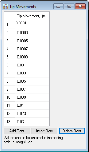

Table F10. TZPILE obtained load-settlement curve.
| Pile Head Load, P, [kN] | Pile Head Movement, δ, [m] |
| 0.0 | 0.000 |
| 920.0 | 0.005 |
| 1576.9 | 0.010 |
| 1922.2 | 0.014 |
| 2148.3 | 0.016 |
| 2233.8 | 0.017 |
| 2353.9 | 0.019 |
| 2727.7 | 0.025 |
| 2854.3 | 0.028 |
| 2888.5 | 0.030 |
| 2898.9 | 0.032 |
| 2904.3 | 0.034 |
| 2939.9 | 0.047 |
| 2941.0 | 0.054 |


Step 10: Identify the location and settlement of the neutral plane (from the soil settlement-pile settlement curve)
The amount of elastic compression within the pile was automatically calculated in the TZPILE software program. These automatically generated values simplify efforts compared to the hand calculation that was presented in Design Example 1. Just like Design Example 1, the TZPILE elastic compression calculations are based on the amount of calculated load within the pile at each incremental depth. The calculated pile settlement was included as Figure F11b, as shown previously. From Figure F11b, the neutral plane that was obtained from the soil settlement-pile settlement curve was 13.78m. The location of the neutral plane as obtained from the combined load-resistance curve and from the soil settlement-pile settlement curve were identical (13.78m). The amount of settlement of the neutral plane (downdrag) was 0.0574m.
Step 11: Perform limit state checks
Limit state checks were performed to determine if the pile size was suitable for the design loads. For the structural strength limit state, the determined drag load (339kN) was multiplied by the drag load factor (γDR=1.1) to obtain a factored load of drag load 373kN. The unfactored top load (2225kN) placed on the top of the pile was multiplied by the deadload factor (γD=1.25) to obtain a factored deadload of 2781kN. The combined total factored load was 3154kN. The concrete compressive strength for the pre-stressed concrete pile was assumed to be 5000psi (34474kPa) resulting in a factored structural stress of 25856kPa (0.75*34474kPa) and a factored structural strength of 3749kN when the stress was multiplied by the cross-sectional area of the pile (0.145m2). If a concrete compressive strength of 5000psi (34474kPa) is used for the pre-stressed pile then the pile is adequately sized because the factored structural strength (3749kN) was determined to be greater than the combined total factored load (3154kN). If a lower-strength concrete was used for the pre-stressed concrete pile, then the pile would need to be larger in cross-sectional area or lengthened. Either type of modification to the pile would result in a change in the amount of drag load on the pile; Steps 3 through 11 of the NCHRP12-116A flowchart would need to be repeated to ensure the factored structural strength was greater than the total factored load for the pile being designed.
Conclusion:
The amount of downdrag and drag load were determined for a pile subjected to ground water lowering. Specifically, the downdrag and drag load were determined by following the 11 steps within the Method B flowchart proposed by the NCHRP12-116A project team. The amount of downdrag was 0.0574m and the amount of drag load was 339kN. The location of the neutral plane was identified to be at a depth of 13.78m. Based on the analysis, the designed pile was adequate for supporting the design loads, including the imposed drag load.
References
Bohn, C., Lopes dos Santos, A., and Frank, R. (2017). “Development of Axial Pile Load Transfer Curves Based on Instrumented Load Tests.” Journal of Geotechnical and Geoenvironmental Engineering 143 (1): 04016081.
Briaud, J.L., and Tucker, L. (1997). NCHRP Report 393: Design and Construction Guidelines for Downdrag on Uncoated and Bitumen-Coated Piles. TRB, National Research Council, Washington, DC.
DeCock, F.A. (2009). “Sense and Sensitivity of Pile Load-Deformation Behavior.” Deep Foundation on Board and Auger Piles. Taylor and Francis. 22 pp.
Ensoft, Inc. (2021). TZPILE Technical Manual. Version 2021. Ensoft, Inc. Austin, TX. 74 pp.
Randolph, M.F., and Murphy, B.S. (1985). “Shaft Capacity of Driven Piles in Clay.” Proceedings of the 1985 Offshore Technology Conference. Paper No. OTC-4883-MS. May 6-9. Houston, TX.
Vijayvergiya, V.N. (1977). “Load-Movement Characteristics of Piles.” Ports ‘77: 4th Annual Symposium of the Waterway, Port, Coastal, and Ocean Division: 269–284. ASCE.


