Page 150

Suggested Citation: "Appendix G: Design Example 5 - Liquefaction in Sand (H-Pile) Using ALLCPT and TZPILE." National Academies of Sciences, Engineering, and Medicine. 2024. Pile Design for Downdrag: Examples and Supporting Materials. Washington, DC: The National Academies Press. doi: 10.17226/27864.

APPENDIX G

Design Example 5 — Liquefaction in Sand (H-Pile) Using ALLCPT and TZPILE

The Boulanger and Idriss (2014) cone penetration test (CPT)-based liquefaction-triggering method, coupled with the Yoshimine et al. (2006) post-liquefaction settlement estimation method as adapted by Idriss and Boulanger (2008), is presented in this CPT-based example calculation of liquefaction-induced settlement. After calculating the liquefaction-induced settlement, the soil settlement was then used to obtain the magnitude of downdrag and drag load by means of the Laboratories des Ponts et Chaussess method (Bustamante and Gianeselli 1982). The estimate of post-liquefaction reconsolidation settlement is driven by the factor of safety against liquefaction triggering, FS_L. Deterministic liquefaction-triggering calculation methods commonly link initial liquefaction to an excess pore pressure ratio of 100% (and/or cyclic shear strain of 3%) corresponding to FS_L = 1.0. However, it is critical to recognize that FS_L > 1.0 does not mean that excess pore pressures have not been generated under strong ground motion. Volumetric strains can accumulate within a soil deposit for FS_L up to 2.0 as shaking generated excess pore pressures dissipate. Thus, seismic design scenario-based liquefaction-triggering calculations, which indicate that liquefaction will not be triggered (i.e., FS_L > 1.0), do not justify the omission of reconsolidation settlement calculations when considering adverse effects to transportation infrastructure.

Discussion of liquefaction susceptibility for CPT-based analyses

The calculation procedure for 1D reconsolidation settlement is directly linked to FS_L for soils that are susceptible to liquefaction. Soils that are not susceptible to liquefaction will need to be evaluated for the potential of cyclic softening, as very soft to medium stiff plastic soils may generate excess pore pressures in the design seismic scenario to result in volumetric strain upon dissipation of excess pore pressures (e.g., Jana and Stuedlein 2021, Dadashiserej et al. 2024). The design engineer must decide how to judge liquefaction susceptibility, which may include selection of a threshold soil behavior type index, I_c, or by comparison of stratigraphic units and the results of laboratory tests from samples retrieved from nearby borings, or both (the preferred methodology). For CPT-based liquefaction-triggering analyses, it is common to select a threshold I_c for which soil is assumed susceptible to liquefaction. Historically (Youd et al. 2001, Zhang et al. 2002), the threshold suggested for use in identifying liquefaction-susceptible soils has been I_c < 2.6, with caution given that soils with Ic ≥ 2.6 can often be sampled in an intact state and as such, should be sampled for cyclic laboratory testing and assessment of the potential for liquefaction or cyclic softening under seismic loading and corresponding volumetric strain potential. It is increasingly being recognized that I_c = 2.6 represents the median of a statistical distribution of I_c for which soils should be screened for liquefaction susceptibility (Stuedlein et al. 2023). Thus, it is recommended that CPTs be paired with nearby boreholes so that samples can be inspected and tested in the laboratory to develop

Page 151

Suggested Citation: "Appendix G: Design Example 5 - Liquefaction in Sand (H-Pile) Using ALLCPT and TZPILE." National Academies of Sciences, Engineering, and Medicine. 2024. Pile Design for Downdrag: Examples and Supporting Materials. Washington, DC: The National Academies Press. doi: 10.17226/27864.

site-specific fines content-I_c correlations and select appropriate I_c thresholds for use with liquefaction-triggering analyses and the consequences of liquefaction (e.g., reconsolidation settlement). Discussions of contemporary views and recent research on the subject of liquefaction susceptibility were presented at a workshop sponsored by the Pacific Earthquake Engineering Research Center and are described in Stuedlein et al. (2023).

Prior to determining I_c, the effective overburden pressure must be calculated to stress-normalize the cone tip and sleeve friction resistance values. In the absence of laboratory-derived unit weights, γ, the effective overburden pressure (σ′_vo ) can be calculated using a correlated unit weight from CPT measurements (Equation 1), using (Robertson and Cabal 2015).

γ = γ_{w} \cdot [0.27 (log R_{f}) + 0.36 (log \frac{q_{t}}{P_{a}}) + 1.236]

Equation 1

In Equation 1, R_f is the friction ratio, defined as the ratio of sleeve resistance to corrected cone resistance, (f_s/q_t) x 100%, γ_w is unit weight of water, and P_a is atmospheric pressure in the same units as q_t (the cone tip resistance).

The soil behavior type index is computed iteratively using Equation 2.

I_{c} = {({(0.34 - log Q_{t})}^{2} + {(log F_{r} + 1.22)}^{2})}^{0.5}

Equation 2

In Equation 2, Q_t is the normalized, corrected net cone penetration resistance, given by (q_t − σ_vo)/σ′_vo and F_r is the normalized friction ratio in percent. The initial I_c value is then recomputed iteratively with an updated, normalized corrected net cone tip resistance, Q_tn, using Equation 3. The initial stress normalization exponent (n) is presented in Equation 4.

Q_{t n} = (\frac{Q_{t} - σ_{ν 0}}{P_{a}}) {(\frac{P_{a}}{{σ^{'}}_{v 0}})}^{n}

Equation 3

n = 0.38 I_{c} + 0.05 (\frac{{σ^{'}}_{v 0}}{P_{a}}) - 0.15 \leq 1

Equation 4

The calculation of I_c, n, and Q_tn is iterated until ∆n ≤ 0.01. Once n has converged, I_c is considered final.

Liquefaction triggering

The factor of safety against liquefaction is computed as the ratio of resistance (i.e., capacity) to demand (loading), in which resistance is represented by the cyclic resistance ratio, CRR, and loading is represented using the cyclic stress ratio, CSR. Owing to the inability to reliably sample many liquefaction-susceptible soils, the triggering calculations typically rely on CRR, which are correlated to penetration resistance or shear wave velocity. Penetration resistance must be corrected to account for the effects of fines content and overburden stresses. For liquefaction-triggering evaluations using the CPT and the Boulanger and Idriss (2014) method, the procedure to correct cone tip resistance is an iterative calculation readily accomplished using spreadsheet solutions. However, the option to perform iterative calculations must be enabled within the spreadsheet. First, the overburden stress-corrected cone tip resistance, q_c1N, is computed using Equation 5.

q_{c 1 N} = C_{N} \frac{q_{c}}{P_{a}}

Equation 5

Page 152

Suggested Citation: "Appendix G: Design Example 5 - Liquefaction in Sand (H-Pile) Using ALLCPT and TZPILE." National Academies of Sciences, Engineering, and Medicine. 2024. Pile Design for Downdrag: Examples and Supporting Materials. Washington, DC: The National Academies Press. doi: 10.17226/27864.

Within Equation 5, C_N is the overburden correction factor and q_cis the unequal area-corrected cone tip resistance (using the area ratio and excess pore pressure measured behind the cone tip). For this analysis, the overburden correction factor for q_c1N is different than the C_N used to calculate Ic (Equation 6). In Equation 6, σ′_v0 is the vertical effective stress at the depth of interest and the exponent m captures the dependence of relative density on the overburden stress-corrected cone tip resistance. The q_c1Ncs is the clean sand and overburden stress-corrected cone tip resistance, to be computed subsequently as part of the iterative calculation. Boulanger and Idriss (2014) state that q_c1Ncs must be limited to the range 21-254 in these computations.

C_{N} = {(\frac{P_{a}}{{σ^{'}}_{v o}})}^{m} \leq 1.7

Equation 6

m = 1.338 - 0.249 {(q_{c 1 N c s})}^{0.264}

Equation 7

The increment in cone tip resistance, ∆q_c1N, stemming from nonzero nonplastic silty fines, which are more compressible than clean sands and yield lower cone tip resistances at a given relative density as a result, is obtained using Equation 8. FC in Equation 8 is the fines content in percent. Here, it is critical to ascertain the plasticity of fines from split-spoon or intact tube samples, as plasticity serves to increase the cyclic resistance of the material. For nonplastic silty fines and the CPT-based liquefaction-triggering assessment, the fines content may be correlated to the soil behavior type index, I_c, using a site-specific correlation (preferred) or the global correlation proposed by Boulanger and Idriss (2014) that is presented as Equation 9. The final step in the iteration is to compute the clean sand and overburden stress-corrected cone tip resistance using Equation 10. The standardized cyclic resistance corresponding to a moment magnitude, M_w, earthquake of 7.5, with 15 uniform shear stress cycles, N = 15, and one atmosphere of pressure may then be computed using Equation 11.

Δ q_{c 1 n} = (11.9 + \frac{q_{c 1 N}}{14.6}) exp (1.63 - \frac{9.7}{F C + 2} - {(\frac{1.57}{F C + 2})}^{2})

Equation 8

F C = 80 I_{c} - 137

Equation 9

q_{c 1 N c s} = q_{c 1 N} + Δ q_{c 1 N}

Equation 10

C R R_{M_{w} = 7.5, {σ^{'}}_{v o} = 1 atm} = exp (\frac{q_{c 1 N c s}}{113} + {(\frac{q_{c 1 N c s}}{1000})}^{2} - {(\frac{q_{c 1 N c s}}{140})}^{3} + {(\frac{q_{c 1 N c s}}{137})}^{4} - 2.80)

Equation 11

The standardized cyclic resistance must then be scaled to vertical effective overburden stresses which exist at the depth where the cone tip resistance was measured and to the design scenario earthquake magnitude. Magnitude scaling essentially accounts for the duration of seismic loading and thus the number of uniform shear stress cycles assumed to be contained within the design ground motion. The correction to CRR effectively results in an increase in resistance for earthquake magnitudes smaller than 7.5, and a decrease in CRR for earthquake magnitudes larger than 7.5. The magnitude scaling factor, MSF, for sandy soils is computed using Equation 12.

M S F = 1 + (M S F_{m a x} - 1) (8.64 exp (- \frac{M}{4}) - 1.325)

Equation 12

The upper bound on magnitude scaling, MSF_max in Equation 12 represents the small-magnitude earthquakes for which the loading may be represented by a fraction of one cycle or one cycle of loading

Page 153

Suggested Citation: "Appendix G: Design Example 5 - Liquefaction in Sand (H-Pile) Using ALLCPT and TZPILE." National Academies of Sciences, Engineering, and Medicine. 2024. Pile Design for Downdrag: Examples and Supporting Materials. Washington, DC: The National Academies Press. doi: 10.17226/27864.

(i.e., a single pulse). The relationship between CRR and N depends on the relative density of sands. Therefore, Boulanger and Idriss (2014) extended the Idriss (1999) magnitude scaling relationship to include q_c1Ncs, which is captured in MSF_max (Equation 13). The correction to cyclic resistance for overburden stress is provided in Equation 14. The C_σ in Equation 14 is determined using Equation 15.

M S F_{m a x} = 1.09 + {(\frac{q_{1 c N c s}}{180})}^{3} \leq 2.2

Equation 13

K_{σ} = 1 - C_{σ} ln (\frac{{σ^{'}}_{v 0}}{P_{q}}) \leq 1.1

Equation 14

C_{σ} = \frac{1}{37.3 - 8.27 {(q_{1 c N c s})}^{0.264}} \leq 0.3

Equation 15

The cyclic resistance for a given magnitude earthquake and overburden stress (i.e., depth) is then scaled from the standardized cyclic resistance using Equation 16. In the “Simplified Method” for liquefaction-triggering evaluation, the effective loading imposed by shear waves is taken equal to 65 percent of the maximum shear stress, τ_max, and is provided in Equation 17. In Equation 17, σ_v0 is the total vertical overburden stress, a_max/g is the peak ground acceleration at the ground surface as a fraction of the gravitational constant, and r_d is the shear stress reduction coefficient to account for “flexibility” of the soil column relative to the rigid block model adopted by Seed and Idriss (1971), as determined using Equation 18.

C R R_{M_{w}, {σ^{'}}_{v 0}} = C R R_{M_{w} = 7.5, {σ^{'}}_{v 0} = 1 atm} \cdot M S F \cdot K_{σ}

Equation 16

C S R_{M_{w}, {σ^{'}}_{v 0}} = 0.65 \frac{τ_{m a x}}{{σ^{'}}_{v 0}} = 0.65 \frac{σ_{v 0}}{{σ^{'}}_{v 0}} \frac{a_{m a x}}{g} r_{d}

Equation 17

r_{d} (z) = exp (α (z) + β (z) \cdot M_{w})

Equation 18

The α(z) and β(z) terms are determined using Equations 19 and 20, respectively, with z being the depth in meters, and the elements encapsulated within the parenthesis are in radians. The factor of safety against liquefaction triggering (i.e., ru = 100%) may then be determined for the depth of interest using Equation 21.

α (z) = - 1.012 - 1.126 \cdot sin (\frac{z}{11.73} + 5.133)

Equation 19

β (z) = 0.106 - 1.118 \cdot sin (\frac{z}{11.28} + 5.142)

Equation 20

F S_{L} = \frac{C R R_{M_{w}, {σ^{'}}_{v 0}}}{C S R_{M_{w}, {σ^{'}}_{v 0}}}

Equation 21

In addition to those described above, other corrections to cyclic resistance also exist. One such example includes corrections to account for soil aging (Andrus et al. 2009); these corrections are particularly useful in Pleistocene deposits. Other potential corrections may be used to account for partial saturation (e.g., Hossein et al. 2013). These corrections are particularly useful in silty sands and nonplastic silts which may exhibit partial saturation below the static groundwater table. Further, efforts to use thin layer-corrected cone tip resistances (e.g., Boulanger and DeJong 2018), corrections for partial saturation, and site-specific CPT-based fines content (FC) correlations have been shown to result in more accurate (and smaller) post--

Page 154

Suggested Citation: "Appendix G: Design Example 5 - Liquefaction in Sand (H-Pile) Using ALLCPT and TZPILE." National Academies of Sciences, Engineering, and Medicine. 2024. Pile Design for Downdrag: Examples and Supporting Materials. Washington, DC: The National Academies Press. doi: 10.17226/27864.

liquefaction reconsolidation settlements when computed for the Avondale Playground case history site in Christchurch, New Zealand (Cary et al. 2022).

Post-liquefaction reconsolidation settlement

Settlement of the ground surface following seismic loading can result from two distinct phenomena: (1) seismic compression of dry and partially-saturated soils (e.g., Duku et al. 2008), and (2) settlement associated with dissipation of excess pore pressures generated in near-saturated and saturated soils (Lee and Albaisa 1974, Ishihara and Yoshimine 1992). For example, seismic compression has been observed to produce settlement in compacted fills following the 1994 Northridge earthquake (Stewart et al. 2002). The resulting ground movements may impact pile foundations through transfer of drag loads during shaking, depending on the relative density and depth of the soil, hypocentral distance, and intensity and duration of loading. Seismic compression is not considered in the example of earthquake-induced settlement described below, which focuses solely on one-dimensional reconsolidation settlement. When computing one-dimensional reconsolidation settlement for a given exploration, it must be recognized that the estimate pertains only to the location of the exploration considered. Care must be taken to place the computed estimate within the context of spatial variability of the stratigraphy (i.e., azimuthal extent and thickness) and the properties within a given unit (Bong and Stuedlein 2018). Furthermore, as noted above, it must be emphasized that reconsolidation settlement occurs as a result of the dissipation of excess pore pressures and as such must be estimated even when FS_L > 1.0.

Several methods are available to estimate seismically-induced reconsolidation settlement (Zhang et al. 2002; Yoshimine et al. 2006). This example considers the Yoshimine et al. (2006) methodology as implemented by Idriss and Boulanger (2008), which uses a correlation between relative density and q_c1Ncs for ease of use with CPT data. The amount of volumetric strain in cyclic laboratory test specimens has been linked to the relative density of the specimen and the magnitude of excess pore pressure generated during cyclic loading. The excess pore pressure generated is in turn related to the maximum shear strain imposed upon the specimen during loading. Hence, the procedure to estimate reconsolidation settlement from volumetric strain includes the calculation of the limiting and maximum shear strain anticipated for a given soil deposit and seismic event, respectively. The limiting shear strain, γ_lim, is determined using Equation 22. As shown in Equation 23, the maximum shear strain, γ_max, anticipated under a given design loading scenario, is assumed smaller than the shear strain necessary to trigger excess pore pressures if FS_L ≥ 2.0. The maximum shear strain is assumed equal to γ_lim if FS_L ≤ FS_α. The maximum shear strain is calculated using Equation 23 if 2 > FS_L > FS_α, with FS_α being calculated in Equation 24. The value of q_c1Ncs is limited to 69 (q_c1Ncs ≥ 69) when calculating FS_α.

γ_{l i m} = 1.859 \cdot {(2.163 - 0.478 {(q_{c 1 N_{C S}})}^{0.264})}^{3} \leq 0

Equation 22

γ_{m a x} = min (γ_{l i m}, 0.035 (2 - F S_{L}) (\frac{1 - F S_{α}}{F S_{L} - F S_{α}}))

Equation 23

F S_{α} = - 11.74 + 8.34 {(q_{c 1 N_{C S}})}^{0.264} - 1.371 {(q_{c 1 N_{C S}})}^{0.528}

Equation 23

The volumetric strain at a given depth, for a given soil layer depth interval, can then be computed using Equation 25. The increment of settlement associated with the volumetric strain at a given depth, z, may then be computed using Equation 26.

Page 155

Suggested Citation: "Appendix G: Design Example 5 - Liquefaction in Sand (H-Pile) Using ALLCPT and TZPILE." National Academies of Sciences, Engineering, and Medicine. 2024. Pile Design for Downdrag: Examples and Supporting Materials. Washington, DC: The National Academies Press. doi: 10.17226/27864.

ε_{v} = 1.5 \cdot exp (2.551 - 1.147 {(q_{c 1 N_{C S}})}^{0.264}) \cdot min (γ_{m a x}, 0.08)

Equation 25

Δ S (Z) = ε_{v} \cdot Δ z

Equation 26

In Equation 26, ∆z is the increment in depth pertaining to the measured penetration resistance at a given depth. Thereafter, the cumulative settlement representing the one-dimensional reconsolidation settlement at the ground surface is computed as the sum of incremental settlements from the base of the exploration, z_max, using Equation 27.

S_{1 D} = \sum_{z = 0}^{z = z_{m a x}} Δ S (z)

Equation 27

Drag load and downdrag determination

The magnitude of the drag load and downdrag can be computed following the determination of the post-liquefaction reconsolidation soil settlement. In keeping with the Boulanger and Idriss (2014) CPT-based liquefaction-triggering method, a CPT-based drag load and downdrag interpretation method is suggested for use. Specifically, the CPT-based LCPC Method that was developed by Laboratories des Ponts et Chaussess is proposed. As documented in Bustamante and Gianeselli (1982), the LCPC Method is an empirical approach developed from an analysis of static load tests in France. Other researchers (Briaud et al. 1986, Rollins et al. 1999) have used the LCPC Method and have suggested modifications or revisions based on other full-scale load tests. For the problems associated with this NCHRP 12-116A project, the piles are considered as Group II – Driven Piles for determination of end bearing resistance. Likewise, for the side resistance, the piles are considered as Category II A (driven concrete piles) or Category II B (driven steel piles).

According to Bustamante and Gianeselli (1982), the smoothed average of the CPT tip resistance values are used to determine the limit resistance under the point of the pile (Q_L^P). To determine the limit resistance under the point of the pile, the bearing capacity factor (k_c) must be selected from Table G1, and the cross-sectional area of the tip of the pile must be known. An equivalent cone resistance at the level of the pile point (q_ca) must be determined (Equation 28).

Q_{L}^{P} = q_{c a} \cdot k_{c} \cdot \frac{π D^{2}}{4}

Equation 28

The procedure for determining the equivalent cone resistance at the level of the pile point is presented in Figure G1. Values between 1.5D above and 1.5D below the pile tip are averaged to determine the smoothed tip resistance profile (q_ca′) within this interval. Then limits are placed on the CPT tip resistance values within this region. If the CPT tip resistance value is larger than 1.3 times the smoothed value at a given depth, the CPT tip resistance value is limited to 1.3 times the smoothed value. Likewise, if the CPT tip resistance value is smaller than 0.7 times the smoothed value at a given depth, the CPT tip resistance value is limited to 0.7 times the smoothed value for depths between the pile tip and 1.5D above the pile tip. No lower limit is placed on the values between the pile tip and 1.5D below the pile tip. After determining the limited average values (q_c,lim) at each depth, the equivalent cone resistance at the level of the pile point (qca) is the average of all of the q_ca′ or qc,lim values from 1.5D above to 1.5D below the pile tip.

Page 156

Suggested Citation: "Appendix G: Design Example 5 - Liquefaction in Sand (H-Pile) Using ALLCPT and TZPILE." National Academies of Sciences, Engineering, and Medicine. 2024. Pile Design for Downdrag: Examples and Supporting Materials. Washington, DC: The National Academies Press. doi: 10.17226/27864.

Table G1. Bearing capacity factor (kc) for various soil types, pile groups, and cone penetration tip resistance (after Bustamante and Gianeselli, 1982). Units of tons per square foot are also included.

		k_c Factor
Soil Type	CPT Tip Resistance, qc	Group I	Group II
Soft clay and mud	<10 MPa (<9.3 tsf)	0.40	0.5
Moderately compact clay	10 to 50 MPa (9.3 to 46.6 tsf)	0.35	0.45
Silt and loose sand	<50 MPa (<46.6 tsf)	0.40	0.5
Compact to stiff clay and compact silt	>50 MPa (>46.6 tsf)	0.45	0.55
Soft chalk	<50 MPa (<46.6 tsf)	0.20	0.3
Moderately compact sand and gravel	50 to 120 MPa (46.6 to 111.9 tsf)	0.4	0.5
Weathered to fragmented chalk	>50 MPa (>46.6 tsf)	0.2	0.4
Compact to very compact sand and gravel	>120 MPa (>111.9 tsf)	0.3	0.4

***Figure G1. Average and limited CPT tip resistance values used to determine the equivalent cone resistance at the level of the pile point (modified from Silvey 2018).***

When using the LCPC method, the determination of the side friction resistance also requires parameter selection from a table (Table G2). The determination of the unit skin friction is much easier than the aforementioned determination of the equivalent cone resistance at the level of the pile point. The measured CPT tip resistance at each depth (q_c) is used in conjunction with the a_LCPC coefficient from Table G2, for the given soil type and category, to determine the unit side resistance (f_n). No averaging or limits are required when determining the unit skin resistance (Equation 29). Instead, limiting values (like the f_s,max shown in Table G2) are placed on the unit skin resistance after determination of the unit skin resistance.

f_{n} = \frac{q_{c}}{a_{L C P C}} < f_{s, m a x}

Equation 29

Page 157

Suggested Citation: "Appendix G: Design Example 5 - Liquefaction in Sand (H-Pile) Using ALLCPT and TZPILE." National Academies of Sciences, Engineering, and Medicine. 2024. Pile Design for Downdrag: Examples and Supporting Materials. Washington, DC: The National Academies Press. doi: 10.17226/27864.

Table G2. Side resistance factors for the LCPC method (after Bustamante and Gianeselli, 1982).

Soil Type	q_c [MPa]	a_LCPC				Limiting value of f_s,max [MPa]
		Category
		I		II		I		II		III
		IA	IB	IIA	IIB	IA	IB	IIA	IIB	IIIA	IIIB
Soft clay and mud	<1	30	30	30	30	0.015	0.015	0.015	0.015	0.015
Moderately compact clay	1 to 5	40	80	40	80	0.08 to 0.035	0.08 to 0.035	0.08 to 0.035	0.035	0.08	>0.120
Silt and loose sand	<5	60	150	60	120	0.035	0.035	0.035	0.035	0.08
Compact to stiff clay and compact silt	>5	60	120	60	120	0.08 to 0.035	0.08 to 0.035	0.08 to 0.035	0.035	0.08	>0.2
Soft chalk	<5	100	120	100	120	0.035	0.035	0.035	0.035	0.08
Moderately compact sand and gravel	5 to 12	100	200	100	200	0.12 to 0.08	0.08 to 0.035	0.12 to 0.08	0.08	0.12	>0.2
Weathered to fragmented chalk	>5	60	80	60	80	0.15 to 0.12	0.12 to 0.08	0.15 to 0.12	0.12	0.15	>0.2
Compact to very compact sand and gravel	>12	150	300	150	200	0.15 to 0.12	0.12 to 0.08	0.15 to 0.12	0.12	0.15	>0.2

The procedure for calculating the amount of drag load after determining the end bearing resistance and side resistance is similar to the approach presented in the later steps of the previous three examples. Like Steps 5, 6, and 7 of Design Example 1, the depth-varying load profile for the pile, the depth-varying resistance profile for the pile, and the combined load and resistance graphs are developed. As previously shown, these graphs are developed by summing the side resistance from the top of the pile to the bottom of the pile (load profile) and by summing the side resistance from the bottom of the pile to the top of the pile (resistance profile). For the load profile, the amount of unfactored top load is added to all of the values of load. Likewise, for the resistance profile, the amount of unfactored end bearing resistance is added to all values of resistance. The combined load and resistance profile is developed by taking the minimum value of load or resistance, at each depth, for all depths. The amount of drag load in the pile is determined by subtracting the unfactored top load from the maximum value of the combined load and resistance curve. The amount of elastic compression in the pile is calculated using the load within the pile (Q above the neutral plane and R below the neutral plane), the cross-sectional area of the pile (A), the elastic modulus of the pile (E), and the segmental length of the pile (L_s). Specifically, the elastic compression for each segment (δ_EC,s) of the pile is determined using Equation 30. The cumulative elastic compression in the pile is then determined by accumulating each of the elastic compression values from the bottom of the pile to the top of the pile (Equation 31). As with Design Example 1, the amount of tip movement of the pile and the nominal compression resistance of the pile can be determined using the DeCock (2009) method based on Chin’s Hyperbolic Model and the Davisson Method (Davisson, 1972), respectively.

δ_{E C, s} = \frac{(M i n [\begin{matrix} Q \\ R \end{matrix}]) L_{s}}{A E}

Eqn. 30

δ_{E C} = Σ (δ_{E C, s}) | from toe of pile to top of pile

Eqn. 31

Page 158

Suggested Citation: "Appendix G: Design Example 5 - Liquefaction in Sand (H-Pile) Using ALLCPT and TZPILE." National Academies of Sciences, Engineering, and Medicine. 2024. Pile Design for Downdrag: Examples and Supporting Materials. Washington, DC: The National Academies Press. doi: 10.17226/27864.

After determining the amount of tip movement and the amount of elastic compression, the pile settlement profile can be developed. The location of the neutral plane can then be determined by plotting the pile settlement profile and the soil settlement profile on the same plot. The location where the pile settlement profile and the soil settlement profile intersect is the location of the neutral plane. Moreover, the amount of movement of the pile and soil at the location of the neutral plane is the amount of downdrag expected for the pile.

The aforementioned methodology can be completed using hand calculations in a manner similar to Design Examples 1 and 3 or through the use of the Ensoft TZPILE program, as used for Design Example 4. Other software programs can also aid in the completion of the aforementioned LCPC Method. Use of the Innovative Geotechnics ALLCPT software program for performing the LCPC Method was utilized herein. Specifically, design calculations and a program tutorial for using the ALLCPT program (NCHRP12-116A Method A) along with the TZPILE program (NCHRP 12-116A Method B) are included in the worked example that is included in the next section. The Method A and Method B flowcharts are provided on the next two pages for completeness.

Worked Example

Step 1: Establish soil data

The following calculation of post-seismic reconsolidation settlement, downdrag determination, and drag load determination was completed for a site along the Mississippi River in Blytheville, Arkansas. The subsurface at this site consists of soft to medium stiff fine-grained soils overlying medium dense to very dense coarse-grained soils. Specifically, the stratigraphy includes 10 feet of soft clay overlying 10 to 15 feet of interbedded, medium-dense, clean and silty sand, overlying 10 feet of medium-dense clean sand, underlain by a thick stratum of dense to very dense sand. The water table was observed to range from a depth of 0 to 10 feet over the course of a year, with a depth of one foot below the ground surface being inferred from the CPT u2 measurements at the time of the sounding. The average CPT data from the site (based on five CPT soundings) are provided in Table G3; the interpreted subsurface conditions encountered at the site are presented in Figure G2. For simplicity in reporting, only every sixth line of the CPT data is presented. The CPT data were scalped using the OFFSET command in Microsoft Excel to obtain every sixth line. Therefore, the interval shown is every 0.984 feet (0.30m) instead of every 0.164 feet (0.05m).

Step 2: Determine soil settlement

The seismic hazards for the design centers on two design events: (1) Event 1, PGA = 0.1g and M_w = 6.5; and (2) Event 2, PGA = 0.4g and M_w = 7.7. Detailed calculations of the factor of safety against liquefaction and 1D reconsolidation settlement for both events are presented for a depth of approximately 25 ft (24.93 ft) below the ground surface. At this location, σ_v0 = 2,758 psf, σ′_v0 = 1,263 psf, and CPT outputs used for the example calculations are presented in Figure G2.

Page 159

Suggested Citation: "Appendix G: Design Example 5 - Liquefaction in Sand (H-Pile) Using ALLCPT and TZPILE." National Academies of Sciences, Engineering, and Medicine. 2024. Pile Design for Downdrag: Examples and Supporting Materials. Washington, DC: The National Academies Press. doi: 10.17226/27864.

presentation

Page 160

Suggested Citation: "Appendix G: Design Example 5 - Liquefaction in Sand (H-Pile) Using ALLCPT and TZPILE." National Academies of Sciences, Engineering, and Medicine. 2024. Pile Design for Downdrag: Examples and Supporting Materials. Washington, DC: The National Academies Press. doi: 10.17226/27864.

Page 161

Suggested Citation: "Appendix G: Design Example 5 - Liquefaction in Sand (H-Pile) Using ALLCPT and TZPILE." National Academies of Sciences, Engineering, and Medicine. 2024. Pile Design for Downdrag: Examples and Supporting Materials. Washington, DC: The National Academies Press. doi: 10.17226/27864.

Table G3. Average CPT sounding record for the Blytheville, AR Test Site.

z	f_s	q_t	u₂	Comments: z=Depth [ft], f_s=Sleeve friction [tsf], q_t=Tip resistance [tsf], u₂=Pore pressure [psi] Values collected every _z=0.164ft but reported herein every _z=0.984ft (except for first and last values).
0.163	0.163	5.990	-0.080
1.148	0.343	6.644	-4.346
2.133	0.321	5.024	-3.507
3.117	0.232	30.509	-0.474
4.101	0.283	8.452	0.052
5.085	0.259	3.602	1.817
6.070	0.279	4.583	2.308
7.054	0.321	5.619	3.310
8.038	0.314	7.221	3.799
9.022	0.178	4.880	4.400
10.007	0.153	26.554	4.783
10.991	0.283	55.585	4.052
11.975	0.380	57.579	3.349
12.959	0.299	41.164	3.934
13.944	0.332	44.718	1.888
14.928	0.412	80.277	0.862
15.912	0.485	99.291	1.548
16.896	0.549	102.243	3.270
17.881	0.435	82.030	3.717
18.865	0.413	81.470	3.345
19.849	0.259	50.410	3.707
20.833	0.233	30.238	3.041
21.818	0.294	56.976	4.014
22.802	0.274	48.270	7.523
23.786	0.306	58.057	7.823
24.770	0.316	59.929	8.438
25.755	0.303	59.692	9.553
26.739	0.271	53.975	11.429
27.723	0.290	60.599	11.954
28.707	0.307	68.630	12.150
29.692	0.328	76.193	13.576
30.676	0.350	86.086	13.470
31.660	0.336	89.231	14.176
32.644	0.419	98.042	15.180
33.629	0.396	96.314	15.467
34.613	0.372	107.343	15.953
35.597	0.410	113.077	16.297
36.581	0.508	143.899	16.744
37.566	0.666	185.609	16.821
38.550	0.608	179.809	17.287
39.561	0.656	185.487	17.292
40.546	0.840	206.957	17.771
41.530	0.866	205.632	16.569
42.569	0.925	210.830	18.586
43.553	0.995	232.122	18.903
44.537	1.028	245.359	19.529
45.549	1.077	259.473	19.777
46.533	1.035	227.953	20.100
47.517	1.000	211.495	20.318
48.529	0.967	220.913	20.881
49.513	1.070	253.789	20.833
50.498	0.895	268.331	21.315
51.482	0.757	256.276	21.870
52.466	0.680	247.751	22.581

Page 162

Suggested Citation: "Appendix G: Design Example 5 - Liquefaction in Sand (H-Pile) Using ALLCPT and TZPILE." National Academies of Sciences, Engineering, and Medicine. 2024. Pile Design for Downdrag: Examples and Supporting Materials. Washington, DC: The National Academies Press. doi: 10.17226/27864.

z	f_s	q_t	u₂	Comments: z=Depth [ft], f_s=Sleeve friction [tsf], q_t=Tip resistance [tsf], u₂=Pore pressure [psi] Values collected every _z=0.164ft but reported herein every _z=0.984ft (except for first and last values).
53.450	0.717	240.933	22.914
54.435	0.653	219.256	23.600
55.474	0.648	245.683	24.005
56.458	0.688	250.659	24.232
57.442	0.767	245.872	24.346
58.481	0.847	268.145	25.168
59.465	1.130	329.023	25.588
60.449	1.317	379.164	25.735
61.488	1.457	392.789	24.920
62.473	1.366	378.497	26.585
63.457	1.462	393.080	26.816
64.469	1.218	375.347	27.283
65.518	1.017	343.502	27.677
66.503	1.156	355.590	28.325
67.626	1.355	342.052	29.154
68.611	0.844	311.256	29.417
69.595	0.687	298.517	29.799
70.579	0.727	290.580	30.460
71.563	0.842	289.159	30.683
72.548	0.729	249.830	31.720
73.710	0.863	273.813	31.332
74.694	0.901	348.687	31.865
75.678	1.635	376.848	31.968
77.018	0.980	322.823	32.031
78.002	0.885	260.040	28.425
78.986	1.091	375.017	32.978
79.970	0.986	345.087	32.455
80.955	0.788	374.134	33.192
81.939	1.274	374.530	34.805
82.923	1.856	404.210	33.297
83.661	1.557	351.657	29.414

Page 163

Suggested Citation: "Appendix G: Design Example 5 - Liquefaction in Sand (H-Pile) Using ALLCPT and TZPILE." National Academies of Sciences, Engineering, and Medicine. 2024. Pile Design for Downdrag: Examples and Supporting Materials. Washington, DC: The National Academies Press. doi: 10.17226/27864.

Figure G2. Soil profile and average CPT data used in the example calculation.

Soils with I_c ≥ 2.6 were assumed to not be susceptible to liquefaction for demonstration purposes only, and FS_L was set equal to 2.0. Additionally, any soil above the ground water table was assumed to not liquefy. Given that materials with I_c ≥ 2.6 at this site are soft to medium stiff, the potential for cyclic softening and post-shaking reconsolidation strains requires consideration. A sampling and laboratory testing program would be recommended to assess cyclic resistance and reconsolidation strain potential (see Section 2.6 of the NCHRP12-116A Phase IV report).

The results of the liquefaction settlement analysis for Event 1 and Event 2 are presented in Figure G3a and Figure G3b, respectively. For Event 1, liquefaction triggering was not indicated with FS_L > 1.0 for all depths, but 2.5 inches of reconsolidation settlement was predicted due to the dissipation of excess pore pressures which are presumed to have been generated by shaking. For Event 2, liquefaction was indicated for depths ranging from 10 to 37 ft, and reconsolidation settlement of 12.2 inches was calculated. For both events, soil settlements extended to the depth of the dense sand layer (37 ft). As discussed in the next section, these settlement profiles were then used as input parameters to determine the location of the neutral plane and the amount of drag load developed. Detailed procedures and computations for determining the post-liquefaction reconsolidation settlement at a depth of 24.93 ft are provided in Table G4. The post-liquefaction reconsolidation settlement calculations and the amount of cumulative soil settlement, as a function of depth, for all depths are reported in Tables G5 through G7.

Page 164

Suggested Citation: "Appendix G: Design Example 5 - Liquefaction in Sand (H-Pile) Using ALLCPT and TZPILE." National Academies of Sciences, Engineering, and Medicine. 2024. Pile Design for Downdrag: Examples and Supporting Materials. Washington, DC: The National Academies Press. doi: 10.17226/27864.

Figure G3. Soil settlement and factor of safety against liquefaction for (a) Event 1, and (b) Event 2. Note: scale change for the cumulative soil settlement (secondary x-axis) between Event 1 and Event 2.

Page 165

Suggested Citation: "Appendix G: Design Example 5 - Liquefaction in Sand (H-Pile) Using ALLCPT and TZPILE." National Academies of Sciences, Engineering, and Medicine. 2024. Pile Design for Downdrag: Examples and Supporting Materials. Washington, DC: The National Academies Press. doi: 10.17226/27864.

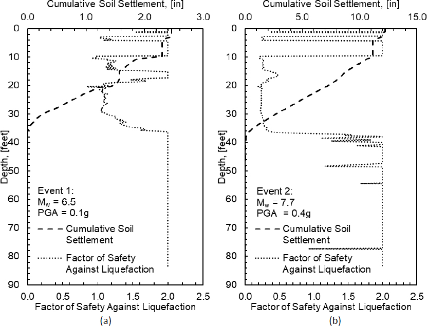
Table G4. Detailed calculations for determining post-liquefaction soil settlement.

*Event 1*
Equation	Worked Example at Depth of 24.93ft	Comment
Calculate the cyclic resistance ratio, CRR
$I_{c} = {({(3.47 - log Q_{t})}^{2} + {(log F_{r} + 1.22)}^{2})}^{0.5}$ $n = 0.38 I_{c} + 0.05 (\frac{{σ^{'}}_{v 0}}{P_{a}}) - 0.15$	$I_{c} = {({(3.47 - log 74.3)}^{2} + {(log 0.528 + 1.22)}^{2})}^{0.5}$ $\begin{matrix} n = 0.38 (1.86) + 0.05 (\frac{1, 263 p s f}{2116 p s f}) - 0.15 \\ = 0.585 \end{matrix}$	Q_tn replaces Q_t in I_c equation following initial calculation. Following iteration (x4): I_c=1.86, n = 0.585, and Q_tn=74.3
FC = 80I_c − 137	FC = 80 ∙ 1.86 − 137 = 11.5%
$q_{c 1 N} = C_{N} \frac{q_{c}}{P_{a}}$ $C_{N} = {(\frac{P_{a}}{{σ^{'}}_{v 0}})}^{m} \leq 1.7$ $m = 1.38 - 24 {(q_{c 1 N c n})}^{0.264}$ $Δ q_{c 1 N} = (11.9 + \frac{q_{c 1 N}}{14.6}) exp (1.63 - \frac{9.7}{F C + 2} - {(\frac{1.57}{F C + 2})}^{2})$ $q_{c 1 N c s} = q_{c 1 N} + Δ q_{c 1 N}$	$q_{1 c N} = 1.32 \frac{59.5 tsf}{1 atm \cdot 1.058 tfs / atm} = 74.0$ $C_{N} = {(\frac{1 atm \cdot 2, 166 psf / atm}{1, 263 psf})}^{0.53} = 1.32$ m = 1.338 − 0.249(85)^0.264 = 0.53 $\begin{matrix} Δ q_{1 c N} = (11.9 + \frac{74.4}{14.6}) exp (1.63 - \frac{9.7}{11.5 + 2} - {(\frac{15.7}{11.5 + 2})}^{2}) \\ = 11 \end{matrix}$ q_c1Ncs = 74.0 + 11.0 = 85.0	Iterative calculation required. Accomplished using the Enable Iterative Calculations option in Excel. To enable the iterative calculations option in Excel, click File > Options > Formulas. Limit q_c1Ncs to the range of [21, 254]

Page 166

Suggested Citation: "Appendix G: Design Example 5 - Liquefaction in Sand (H-Pile) Using ALLCPT and TZPILE." National Academies of Sciences, Engineering, and Medicine. 2024. Pile Design for Downdrag: Examples and Supporting Materials. Washington, DC: The National Academies Press. doi: 10.17226/27864.

$C R R_{M_{w} = 7.5, {σ^{'}}_{v 0} = 1 atm} = exp (\frac{q_{1 c N c s}}{113} + {(\frac{q_{c 1 N c s}}{1000})}^{2} - {(\frac{q_{c 1 N c s}}{140})}^{3} + {(\frac{q_{c 1 N c s}}{137})}^{4} - 2.80)$	$C R R_{M_{w} = 7.5, {σ^{'}}_{v 0} = 1 atm} = exp (\frac{85.0}{113} + {(\frac{85.0}{1000})}^{2} - {(\frac{85.0}{140})}^{3} + {(\frac{85.0}{137})}^{4} - 2.80) = 0.12$
$M S F_{m a x} = 1.09 + {(\frac{q_{c 1 N c s}}{180})}^{3} \leq 2.2$	$M S F_{m a x} = 1.09 + {(\frac{85.0}{180})}^{3} = 1.195$
$M S F = 1 + (M S F_{m a x} - 1) (8.64 exp (- \frac{M}{4}) - 1.325)$	$M S F = 1 + (1.195 - 1) (8.64 exp (- \frac{6.5}{4}) - 1.325) = 1.073$
$C_{σ} = \frac{1}{37.3 - 8.27 {(q_{c 1 N c s})}^{0.264}} \leq 0.3$	$C_{σ} = \frac{1}{37.3 - 8.27 {(85.0)}^{0.264}} = 0.095$
$K_{σ} = 1 - C_{σ} (\frac{{σ^{'}}_{v 0}}{P_{a}}) \leq 1.1$	$K_{σ} = 1 - 0.095 ln (\frac{1, 263 psf}{2, 116 psf}) = 1.05$
$C R R_{M_{w}, {σ^{'}}_{v 0}} = C R R_{M_{w} = 7.5, {σ^{'}}_{v 0} = 1 atm} \cdot M S F \cdot K_{σ}$	$C R R_{M_{w}, {σ^{'}}_{v 0}} = 0.12 \cdot 1.073 \cdot 1.05 = 0.136$
Calculate the cyclic stress ratio, CSR
$α (z) = - 1.012 - 1.126 \cdot sin (\frac{z}{11.73} + 5.133)$	$\begin{array}{l} α (z) = - 1.012 - 1.126 \cdot sin (\frac{\frac{24.93 ft}{3.28 1 m per ft}}{11.73} + 5.133) \\ = - 0.47 \end{array}$

Page 167

Suggested Citation: "Appendix G: Design Example 5 - Liquefaction in Sand (H-Pile) Using ALLCPT and TZPILE." National Academies of Sciences, Engineering, and Medicine. 2024. Pile Design for Downdrag: Examples and Supporting Materials. Washington, DC: The National Academies Press. doi: 10.17226/27864.

$β (z) = 0.106 - 1.118 \cdot sin (\frac{z}{11.28} + 5.142)$	$\begin{array}{l} β (z) = 0.106 - 1.118 \cdot sin (\frac{\frac{24.93 ft}{3.28 1 m per ft}}{11.28} + 5.142) \\ = 0.053 \end{array}$
$r_{d} (z) = exp (α (z) + β (z) \cdot M_{w})$	$r_{d} (z) = exp (- 0.47 + 0.053 \cdot 6.5) = 0.881$
$C S R_{M_{w}, {σ^{'}}_{v 0}} = 0.65 \frac{σ_{v 0}}{{σ^{'}}_{v 0}} \cdot \frac{a_{m a x}}{g} \cdot r_{d}$	$\begin{matrix} C S R_{M_{w}, {σ^{'}}_{v 0}} = 0.65 \frac{2, 758 psf}{1, 263 psf} \cdot \frac{0.1 g}{g} \cdot 0.881 \\ = 0.125 \end{matrix}$
Calculate the factor of safety against liquefaction, FS_L
$F L_{L} = \frac{C R R_{M_{w}, {σ^{'}}_{v o 0}}}{C S R_{M_{w}, {σ^{'}}_{v o 0}}}$	$F S_{L} = \frac{0.135}{0.125} = 1.08$	See Figure G3; FS_L ≤ 2.0 triggers calculation of volumetric strain and corresponding settlement
Calculate reconsolidation settlement
$F S_{α} = - 11.74 + 8.34 {(q_{c 1 N c s})}^{0.264} - 1.371 {(q_{c 1 N c s})}^{0.528}$	$F S_{α} = - 11.74 + 8.34 {(85.0)}^{0.264} - 1.371 {(85.0)}^{0.528}$	Limit q_c1Ncs ≥ 69
$y_{l i m} = 1.859 {(2.163 - 0.478 {(q_{c 1 N c s})}^{0.264})}^{3} \geq 0$	$\begin{matrix} y_{l i m} = 1.859 {(2.163 - 0.478 {(85.0)}^{0.264})}^{3} \\ = 0.44 \end{matrix}$	This is arithmetic strain, equal to γ_lim = 44% and associated with low relative density
$γ_{m a x} = min (γ_{l i m}, 0.035 (2 - F S_{L}) (\frac{1 - F S_{α}}{F S_{L} - F S_{α}}))$	$\begin{matrix} γ_{m a x} = min (0.44, 0.035 (2 - 1.08) (\frac{1 - 0.894}{1.08 - 0.9894})) \\ = 0.018 \end{matrix}$	This is arithmetic strain, equal to γ_max = 1.8% and associated with low PGA
$ε_{v} = 1.5 \cdot exp (2.551 - 1.147 {(q_{c 1 N c s})}^{0.264}) \cdot min (γ_{m a x}, 0.08)$	$ε_{v} = 1.5 \cdot exp (2.551 - 1.147 {(85.0)}^{0.264}) \cdot min (0.018, 0.08) = 0.008$	This is arithmetic strain, equal to ε_v = 0.8%
$Δ s (z) = ε_{v} \cdot Δ z$	$\begin{matrix} Δ s (z) = 0.008 \cdot (0.16 ft) \cdot 12 in per ft \\ = 0.017 in \end{matrix}$
$S_{1 D} = \sum_{z = 0}^{z = z_{m a x}} Δ s (z)$	S_1D = 2.5 inches	See Figure G3.

Page 168

Suggested Citation: "Appendix G: Design Example 5 - Liquefaction in Sand (H-Pile) Using ALLCPT and TZPILE." National Academies of Sciences, Engineering, and Medicine. 2024. Pile Design for Downdrag: Examples and Supporting Materials. Washington, DC: The National Academies Press. doi: 10.17226/27864.

Table G5. Results from calculations to find corrected tip resistance.

z		_vo′	Ic	n	Q_tn	q_c1N	C_N	m	_qc1N	q_c1Ncs	Comments: For Event #1 – a_max=0.1, M_w=6.5, z=Depth [ft], =Unit weight [pcf], _vo–=Vertical effective stress [psf], I_{c=Soil behavior type index, n=stress normalization exponent, Q_tn=Normalized corrected net cone tip resistance, q_c1N=Overburden stress-corrected cone tip resistance [tsf], C_N=Overburden correction factor, m=Overburden correction factor exponent, _qc1N=Increment in cone tip resistance [tsf], q_c1Ncs}=Clean sand and overburden stress-corrected cone tip resistance [tsf]. Values collected every z=0.164ft but reported herein every _z=0.984ft (except for first and last values).
0.163	120.822	19.738	2.190	0.683	137.351	9.624	1.700	0.628	43.214	52.837
1.148	107.801	125.255	2.543	0.819	67.872	10.674	1.700	0.592	53.081	63.755
2.133	105.991	229.496	2.720	0.887	46.606	8.071	1.700	0.596	54.513	62.584
3.117	113.182	338.402	1.837	0.553	104.314	49.018	1.700	0.620	6.153	55.171
4.101	110.548	453.651	2.539	0.821	43.669	13.580	1.700	0.581	53.853	67.433
5.085	103.417	555.312	2.996	0.996	22.063	5.786	1.700	0.599	55.730	61.516
6.070	105.630	658.756	2.924	0.969	23.599	7.363	1.700	0.594	55.970	63.333
7.054	106.426	762.746	2.882	0.954	25.261	9.027	1.700	0.588	56.185	65.212
8.038	107.520	867.675	2.769	0.912	27.638	11.602	1.700	0.580	56.046	67.648
9.022	101.243	969.769	2.880	0.955	17.579	7.841	1.700	0.593	55.809	63.649
10.007	114.235	1074.550	1.971	0.611	58.582	42.662	1.700	0.565	30.473	73.136
10.991	113.878	1188.052	1.729	0.520	103.531	89.305	1.700	0.523	0.000	89.305
11.975	113.888	1299.143	1.785	0.543	105.468	92.510	1.700	0.514	0.488	92.998
12.959	112.948	1411.400	1.925	0.597	76.425	66.136	1.700	0.518	25.361	91.497
13.944	115.292	1522.129	1.917	0.595	79.401	71.846	1.700	0.507	24.349	96.195
14.928	114.023	1635.068	1.662	0.500	124.908	120.641	1.590	0.456	0.000	120.641
15.912	116.185	1748.957	1.593	0.475	146.144	139.982	1.492	0.420	0.000	139.982
16.896	117.133	1864.281	1.614	0.484	147.175	140.264	1.452	0.420	0.000	140.264
17.881	115.266	1978.696	1.693	0.515	117.381	114.269	1.474	0.468	0.000	114.269
18.865	114.686	2091.573	1.694	0.517	113.434	111.183	1.444	0.474	0.000	111.183
19.849	110.400	2201.933	1.871	0.585	71.261	70.255	1.475	0.535	14.012	84.267
20.833	107.996	2306.491	2.144	0.690	44.084	40.910	1.432	0.524	47.842	88.752
21.818	111.073	2414.187	1.845	0.578	76.371	75.895	1.409	0.535	8.632	84.527
22.802	109.488	2522.566	1.933	0.612	64.164	62.479	1.370	0.524	26.522	89.002
23.786	110.799	2630.505	1.860	0.585	74.492	73.952	1.348	0.532	11.743	85.695
24.770	111.341	2740.067	1.857	0.585	75.134	74.755	1.320	0.531	11.049	85.804
25.755	110.547	2849.221	1.858	0.587	73.204	73.119	1.296	0.535	11.296	84.415
26.739	110.086	2957.878	1.901	0.604	65.096	64.819	1.271	0.533	20.286	85.105
27.723	110.588	3067.169	1.856	0.588	71.248	71.631	1.251	0.540	10.844	82.475
28.707	111.897	3176.704	1.804	0.570	78.705	79.730	1.229	0.542	1.790	81.520
29.692	112.653	3286.978	1.764	0.556	85.465	86.551	1.202	0.530	0.026	86.577
30.676	113.638	3397.761	1.713	0.538	94.472	95.483	1.174	0.508	0.000	95.483
31.660	113.003	3509.623	1.691	0.530	96.059	97.256	1.153	0.504	0.000	97.256
32.644	115.062	3621.893	1.688	0.530	103.928	104.746	1.130	0.488	0.000	104.746
33.629	114.899	3734.786	1.693	0.533	100.416	101.522	1.115	0.495	0.000	101.522
34.613	114.591	3847.326	1.622	0.508	109.784	111.068	1.095	0.475	0.000	111.068
35.597	115.863	3961.458	1.618	0.507	113.953	115.207	1.078	0.466	0.000	115.207
36.581	117.757	4076.590	1.526	0.474	142.725	143.622	1.056	0.414	0.000	143.622
37.566	120.242	4194.474	1.440	0.443	181.446	181.864	1.037	0.355	0.000	181.864
38.550	119.499	4312.741	1.444	0.445	173.422	174.495	1.027	0.365	0.000	174.495
39.561	120.083	4434.628	1.447	0.448	176.598	178.041	1.016	0.360	0.000	178.041
40.546	121.871	4553.866	1.445	0.448	194.761	196.572	1.005	0.334	0.000	196.572
41.530	122.199	4674.384	1.461	0.456	191.015	193.487	0.996	0.338	0.000	193.487
42.569	123.445	4802.070	1.468	0.460	193.243	196.480	0.986	0.334	0.000	196.480
43.553	123.941	4923.348	1.432	0.448	210.501	214.749	0.979	0.310	0.000	214.749
44.537	123.910	5045.827	1.410	0.441	220.087	225.413	0.972	0.297	0.000	225.413
45.549	124.236	5171.284	1.392	0.435	230.278	236.911	0.966	0.283	0.000	236.911
46.533	123.506	5293.349	1.467	0.465	198.903	205.483	0.954	0.322	0.000	205.483
47.517	124.343	5415.452	1.509	0.483	181.689	188.407	0.943	0.345	0.000	188.407
48.529	123.000	5540.488	1.477	0.472	188.003	195.521	0.936	0.336	0.000	195.521
49.513	123.547	5662.041	1.420	0.452	214.886	224.721	0.937	0.298	0.000	224.721
50.498	122.997	5783.748	1.342	0.424	226.501	236.827	0.934	0.283	0.000	236.827
51.482	121.750	5903.794	1.335	0.422	214.291	223.896	0.924	0.299	0.000	223.896
52.466	121.018	6022.677	1.335	0.424	205.151	214.395	0.916	0.311	0.000	214.395

Page 169

Suggested Citation: "Appendix G: Design Example 5 - Liquefaction in Sand (H-Pile) Using ALLCPT and TZPILE." National Academies of Sciences, Engineering, and Medicine. 2024. Pile Design for Downdrag: Examples and Supporting Materials. Washington, DC: The National Academies Press. doi: 10.17226/27864.

z		_vo′	Ic	n	Q_tn	q_c1N	C_N	m	_qc1N	q_c1Ncs	Comments: See definition of variables on previous page. Values collected every ∆z=0.164ft but reported herein every ∆z=0.984ft (except for first and last values).
53.450	121.375	6141.791	1.368	0.438	196.831	206.549	0.907	0.321	0.000	206.549
54.435	120.474	6260.247	1.410	0.455	176.321	185.030	0.893	0.350	0.000	185.030
55.474	120.556	6385.614	1.341	0.430	197.683	208.063	0.896	0.319	0.000	208.063
56.458	120.924	6504.888	1.345	0.433	199.820	211.300	0.892	0.315	0.000	211.300
57.442	121.561	6624.140	1.386	0.450	193.053	205.445	0.884	0.322	0.000	205.445
58.481	122.479	6750.393	1.358	0.441	209.641	224.845	0.887	0.298	0.000	224.845
59.465	124.887	6872.280	1.304	0.421	257.745	278.294	0.895	0.264	0.000	254.000
60.449	126.740	6996.671	1.257	0.405	297.100	319.071	0.890	0.264	0.000	254.000
61.488	127.600	7128.689	1.266	0.410	304.597	328.776	0.886	0.264	0.000	254.000
62.473	126.950	7254.346	1.275	0.415	290.399	315.231	0.881	0.264	0.000	254.000
63.457	127.479	7379.282	1.272	0.416	299.257	325.789	0.877	0.264	0.000	254.000
64.469	125.938	7507.147	1.255	0.411	284.171	309.583	0.873	0.264	0.000	254.000
65.518	124.651	7640.161	1.269	0.417	256.807	281.911	0.868	0.264	0.000	254.000
66.503	125.502	7762.766	1.283	0.424	263.053	290.541	0.865	0.264	0.000	254.000
67.626	126.212	7902.300	1.356	0.454	246.692	278.103	0.860	0.264	0.000	254.000
68.611	122.403	8024.086	1.297	0.433	225.304	251.602	0.855	0.267	0.000	251.602
69.595	121.499	8144.146	1.280	0.428	215.142	238.091	0.844	0.282	0.000	238.091
70.579	121.793	8264.421	1.314	0.442	206.152	229.293	0.835	0.292	0.000	229.293
71.563	122.231	8385.033	1.355	0.459	201.555	226.729	0.830	0.296	0.000	226.729
72.548	122.618	8505.017	1.421	0.485	169.611	188.973	0.800	0.344	0.000	188.973
73.710	123.440	8649.010	1.404	0.481	185.100	209.681	0.810	0.317	0.000	209.681
74.694	123.754	8770.369	1.257	0.426	243.712	275.531	0.836	0.264	0.000	254.000
75.678	128.338	8895.132	1.371	0.471	253.916	296.602	0.833	0.264	0.000	254.000
77.018	124.661	9061.838	1.337	0.460	216.689	252.473	0.828	0.266	0.000	252.473
78.002	124.108	9185.051	1.461	0.509	166.798	191.854	0.781	0.341	0.000	191.854
78.986	125.660	9307.667	1.270	0.438	253.122	291.482	0.822	0.264	0.000	254.000
79.970	124.876	9432.607	1.304	0.452	228.713	267.216	0.819	0.264	0.000	254.000
80.955	124.062	9556.417	1.198	0.413	254.053	288.658	0.816	0.264	0.000	254.000
81.939	126.667	9681.199	1.322	0.462	243.412	287.915	0.813	0.264	0.000	254.000
82.923	130.206	9805.708	1.384	0.487	256.159	309.623	0.811	0.264	0.000	254.000
83.661	127.812	10859.659	1.430	0.505	217.688	268.635	0.808	0.264	0.000	254.000

Page 170

Suggested Citation: "Appendix G: Design Example 5 - Liquefaction in Sand (H-Pile) Using ALLCPT and TZPILE." National Academies of Sciences, Engineering, and Medicine. 2024. Pile Design for Downdrag: Examples and Supporting Materials. Washington, DC: The National Academies Press. doi: 10.17226/27864.

Table G6. Results from CRR, cyclic stress ratio, and factor of safety calculations.

z	r_d	(z)	(z)	K	C	MSF_max	MSF	CRR_7.5,1atm	CRR_M,′v	CSR_M,′v	Comments: For Event #1 – a_max=0.1, M_w=6.5, z=Depth [ft], r_d=Shear stress reduction coefficient, (z)=Term used to find r_d, (z)=Term used to find r_d, K= correction to cyclic resistance for overburden stress, C=Term used to find K, MSF_max=Upper bound on magnitude scaling, MSF, CRR_7.5,1atm = standardized cyclic resistance corresponding to a moment magnitude earthquake of 7.5, with 15 uniform shear stress cycles, and one atmosphere of pressure, CRRM,_–v =Cyclic resistance ratio for the magnitude and effective stress of interest, CSRM,_–v=Cyclic stress ratio for the magnitude and effective stress of interest. Values collected every z=0.164ft but reported herein every z=0.984ft (except for first and last values).
0.163	1.00	0.01	0.00	1.10	0.07	1.12	1.04	0.09	0.11	0.07
1.148	1.00	0.00	0.00	1.10	0.08	1.13	1.05	0.10	0.12	0.07
2.133	1.00	-0.01	0.00	1.10	0.08	1.13	1.05	0.10	0.12	0.09
3.117	1.00	-0.02	0.00	1.10	0.07	1.12	1.04	0.10	0.11	0.11
4.101	0.99	-0.04	0.00	1.10	0.08	1.14	1.05	0.11	0.12	0.11
5.085	0.99	-0.05	0.01	1.10	0.08	1.13	1.05	0.10	0.12	0.12
6.070	0.98	-0.07	0.01	1.10	0.08	1.13	1.05	0.10	0.12	0.12
7.054	0.98	-0.09	0.01	1.10	0.08	1.14	1.05	0.10	0.12	0.13
8.038	0.98	-0.10	0.01	1.10	0.08	1.14	1.05	0.11	0.12	0.13
9.022	0.97	-0.12	0.01	1.10	0.08	1.13	1.05	0.10	0.12	0.13
10.007	0.97	-0.14	0.02	1.10	0.09	1.16	1.06	0.11	0.13	0.13
10.991	0.96	-0.16	0.02	1.10	0.10	1.21	1.08	0.12	0.15	0.13
11.975	0.96	-0.17	0.02	1.10	0.10	1.23	1.09	0.13	0.15	0.13
12.959	0.95	-0.19	0.02	1.10	0.10	1.22	1.08	0.13	0.15	0.13
13.944	0.95	-0.21	0.02	1.10	0.10	1.24	1.09	0.13	0.16	0.13
14.928	0.94	-0.23	0.03	1.10	0.13	1.39	1.15	0.17	0.22	0.13
15.912	0.94	-0.26	0.03	1.10	0.15	1.56	1.21	0.23	0.31	0.13
16.896	0.93	-0.28	0.03	1.10	0.15	1.56	1.21	0.24	0.31	0.13
17.881	0.92	-0.30	0.03	1.10	0.12	1.35	1.13	0.16	0.20	0.13
18.865	0.92	-0.32	0.04	1.09	0.12	1.33	1.12	0.15	0.19	0.13
19.849	0.91	-0.34	0.04	1.07	0.09	1.19	1.07	0.12	0.14	0.13
20.833	0.91	-0.37	0.04	1.07	0.10	1.21	1.08	0.12	0.14	0.13
21.818	0.90	-0.39	0.04	1.06	0.09	1.19	1.07	0.12	0.14	0.13
22.802	0.89	-0.42	0.05	1.06	0.10	1.21	1.08	0.12	0.14	0.13
23.786	0.89	-0.44	0.05	1.05	0.10	1.20	1.07	0.12	0.14	0.13
24.770	0.88	-0.47	0.05	1.05	0.10	1.20	1.07	0.12	0.14	0.13
25.755	0.88	-0.49	0.06	1.05	0.09	1.19	1.07	0.12	0.13	0.12
26.739	0.87	-0.52	0.06	1.04	0.09	1.20	1.07	0.12	0.13	0.12
27.723	0.86	-0.54	0.06	1.04	0.09	1.19	1.07	0.12	0.13	0.12
28.707	0.86	-0.57	0.06	1.04	0.09	1.18	1.07	0.12	0.13	0.12
29.692	0.85	-0.60	0.07	1.03	0.10	1.20	1.08	0.12	0.14	0.12
30.676	0.84	-0.62	0.07	1.03	0.10	1.24	1.09	0.13	0.15	0.12
31.660	0.84	-0.65	0.07	1.03	0.10	1.25	1.09	0.13	0.15	0.12
32.644	0.83	-0.68	0.08	1.03	0.11	1.29	1.11	0.14	0.16	0.12
33.629	0.82	-0.70	0.08	1.02	0.11	1.27	1.10	0.14	0.16	0.12
34.613	0.82	-0.73	0.08	1.02	0.12	1.32	1.12	0.15	0.18	0.12
35.597	0.81	-0.76	0.08	1.02	0.12	1.35	1.13	0.16	0.19	0.12
36.581	0.81	-0.79	0.09	1.02	0.15	1.60	1.23	0.25	0.31	0.12
37.566	0.80	-0.82	0.09	1.02	0.22	2.12	1.42	0.78	1.14	0.11
38.550	0.79	-0.85	0.09	1.01	0.20	2.00	1.38	0.59	0.82	0.11
39.561	0.79	-0.87	0.10	1.01	0.21	2.06	1.40	0.67	0.95	0.11
40.546	0.78	-0.90	0.10	1.00	0.25	2.20	1.45	1.57	2.28	0.11
41.530	0.77	-0.93	0.10	1.00	0.24	2.20	1.45	1.33	1.93	0.11
42.569	0.77	-0.96	0.11	0.99	0.25	2.20	1.45	1.56	2.24	0.11
43.553	0.76	-0.99	0.11	0.98	0.30	2.20	1.45	2.00	2.84	0.11
44.537	0.75	-1.02	0.11	0.97	0.30	2.20	1.45	2.00	2.82	0.11
45.549	0.75	-1.05	0.12	0.96	0.30	2.20	1.45	2.00	2.80	0.11
46.533	0.74	-1.08	0.12	0.96	0.28	2.20	1.45	2.00	2.78	0.10
47.517	0.73	-1.11	0.12	0.96	0.23	2.20	1.45	1.04	1.45	0.10
48.529	0.73	-1.14	0.13	0.95	0.25	2.20	1.45	1.48	2.05	0.10
49.513	0.72	-1.17	0.13	0.93	0.30	2.20	1.45	2.00	2.71	0.10
50.498	0.72	-1.19	0.13	0.93	0.30	2.20	1.45	2.00	2.69	0.10
51.482	0.71	-1.22	0.14	0.92	0.30	2.20	1.45	2.00	2.67	0.10
52.466	0.70	-1.25	0.14	0.91	0.30	2.20	1.45	2.00	2.66	0.10

Page 171

Suggested Citation: "Appendix G: Design Example 5 - Liquefaction in Sand (H-Pile) Using ALLCPT and TZPILE." National Academies of Sciences, Engineering, and Medicine. 2024. Pile Design for Downdrag: Examples and Supporting Materials. Washington, DC: The National Academies Press. doi: 10.17226/27864.

z	r_d	(z)	(z)	K	C	MSF_max	MSF	CRR_7.5,1atm	CRR_M,′v	CSR_M,′v	Comments: See definition of variables on previous page. Values collected every ∆z=0.164ft but reported herein every ∆z=0.984ft (except for first and last values).
53.450	0.70	-1.28	0.14	0.91	0.28	2.20	1.45	2.00	2.65	0.10
54.435	0.69	-1.31	0.14	0.93	0.22	2.18	1.44	0.90	1.20	0.10
55.474	0.69	-1.34	0.15	0.90	0.29	2.20	1.45	2.00	2.61	0.10
56.458	0.68	-1.36	0.15	0.89	0.30	2.20	1.45	2.00	2.59	0.09
57.442	0.67	-1.39	0.15	0.89	0.28	2.20	1.45	2.00	2.59	0.09
58.481	0.67	-1.42	0.16	0.88	0.30	2.20	1.45	2.00	2.55	0.09
59.465	0.66	-1.45	0.16	0.87	0.30	2.20	1.45	2.00	2.54	0.09
60.449	0.66	-1.47	0.16	0.87	0.30	2.20	1.45	2.00	2.52	0.09
61.488	0.65	-1.50	0.16	0.86	0.30	2.20	1.45	2.00	2.50	0.09
62.473	0.65	-1.53	0.17	0.86	0.30	2.20	1.45	2.00	2.49	0.09
63.457	0.64	-1.55	0.17	0.85	0.30	2.20	1.45	2.00	2.47	0.09
64.469	0.64	-1.58	0.17	0.85	0.30	2.20	1.45	2.00	2.45	0.09
65.518	0.63	-1.60	0.18	0.84	0.30	2.20	1.45	2.00	2.44	0.09
66.503	0.62	-1.63	0.18	0.83	0.30	2.20	1.45	2.00	2.42	0.09
67.626	0.62	-1.65	0.18	0.83	0.30	2.20	1.45	2.00	2.41	0.08
68.611	0.61	-1.68	0.18	0.82	0.30	2.20	1.45	2.00	2.39	0.08
69.595	0.61	-1.70	0.19	0.82	0.30	2.20	1.45	2.00	2.38	0.08
70.579	0.60	-1.72	0.19	0.81	0.30	2.20	1.45	2.00	2.37	0.08
71.563	0.60	-1.75	0.19	0.81	0.30	2.20	1.45	2.00	2.35	0.08
72.548	0.60	-1.77	0.19	0.85	0.23	2.20	1.45	1.07	1.32	0.08
73.710	0.59	-1.79	0.19	0.80	0.30	2.20	1.45	2.00	2.33	0.08
74.694	0.59	-1.81	0.20	0.80	0.30	2.20	1.45	2.00	2.31	0.08
75.678	0.58	-1.83	0.20	0.79	0.30	2.20	1.45	2.00	2.30	0.08
77.018	0.58	-1.86	0.20	0.79	0.30	2.20	1.45	2.00	2.28	0.08
78.002	0.57	-1.88	0.20	0.83	0.24	2.20	1.45	1.23	1.47	0.08
78.986	0.57	-1.90	0.20	0.78	0.30	2.20	1.45	2.00	2.26	0.08
79.970	0.57	-1.91	0.21	0.77	0.30	2.20	1.45	2.00	2.25	0.08
80.955	0.56	-1.93	0.21	0.77	0.30	2.20	1.45	2.00	2.23	0.08
81.939	0.56	-1.95	0.21	0.77	0.30	2.20	1.45	2.00	2.22	0.08
82.923	0.55	-1.96	0.21	0.76	0.30	2.20	1.45	2.00	2.21	0.08
83.661	0.55	-1.97	0.21	0.76	0.30	2.20	1.45	2.00	2.20	0.08

Page 172

Suggested Citation: "Appendix G: Design Example 5 - Liquefaction in Sand (H-Pile) Using ALLCPT and TZPILE." National Academies of Sciences, Engineering, and Medicine. 2024. Pile Design for Downdrag: Examples and Supporting Materials. Washington, DC: The National Academies Press. doi: 10.17226/27864.

Table G7. Results from Yoshimine et al. (2006) and Idriss and Boulanger (2008) calculations.

z	FS	_lim	_max	_v			Comments: For Event #1 – a_max=0.1, M_w=6.5, z=Depth [ft], FS =Factor of Safety, _lim =Limiting shear strain, _max=Maximum shear strain, _v=Volumetric strain, = _s = Incremental soil settlement [in], = s_1D = Cumulative soil settlement from bottom of soil profile top of soil profile [in]. Values collected every _z=0.164ft but reported herein every z=0.984ft (except for first and last values).
0.163	0.94	0.95	0.00	0.00	0.00	2.46
1.148	0.94	0.73	0.00	0.00	0.00	2.46
2.133	0.94	0.75	0.00	0.00	0.00	2.46
3.117	0.94	0.90	0.02	0.02	0.03	2.43
4.101	0.94	0.67	0.01	0.01	0.02	2.32
5.085	0.94	0.77	0.00	0.00	0.00	2.30
6.070	0.94	0.73	0.00	0.00	0.00	2.30
7.054	0.94	0.70	0.00	0.00	0.00	2.30
8.038	0.94	0.66	0.00	0.00	0.00	2.30
9.022	0.94	0.73	0.00	0.00	0.00	2.30
10.007	0.94	0.58	0.07	0.04	0.08	2.15
10.991	0.87	0.40	0.02	0.01	0.01	1.84
11.975	0.85	0.37	0.01	0.01	0.01	1.77
12.959	0.86	0.38	0.01	0.01	0.01	1.70
13.944	0.82	0.34	0.01	0.01	0.01	1.63
14.928	0.60	0.19	0.00	0.00	0.00	1.58
15.912	0.37	0.12	0.00	0.00	0.00	1.57
16.896	0.37	0.12	0.00	0.00	0.00	1.57
17.881	0.66	0.22	0.01	0.00	0.00	1.57
18.865	0.69	0.24	0.01	0.00	0.01	1.54
19.849	0.90	0.45	0.02	0.01	0.02	1.47
20.833	0.87	0.40	0.02	0.01	0.01	1.20
21.818	0.90	0.44	0.02	0.01	0.02	1.09
22.802	0.87	0.40	0.02	0.01	0.01	0.98
23.786	0.89	0.43	0.02	0.01	0.02	0.89
24.770	0.89	0.43	0.02	0.01	0.02	0.80
25.755	0.90	0.45	0.02	0.01	0.02	0.70
26.739	0.89	0.44	0.02	0.01	0.02	0.61
27.723	0.91	0.47	0.02	0.01	0.02	0.51
28.707	0.91	0.48	0.02	0.01	0.02	0.40
29.692	0.89	0.42	0.02	0.01	0.01	0.28
30.676	0.83	0.34	0.01	0.00	0.01	0.21
31.660	0.81	0.33	0.01	0.00	0.01	0.15
32.644	0.75	0.28	0.01	0.00	0.01	0.11
33.629	0.78	0.30	0.01	0.00	0.01	0.07
34.613	0.69	0.24	0.01	0.00	0.00	0.03
35.597	0.65	0.22	0.01	0.00	0.00	0.01
36.581	0.33	0.11	0.00	0.00	0.00	0.00
37.566	-0.19	0.04	0.00	0.00	0.00	0.00
38.550	-0.08	0.05	0.00	0.00	0.00	0.00
39.561	-0.13	0.04	0.00	0.00	0.00	0.00
40.546	-0.40	0.02	0.00	0.00	0.00	0.00
41.530	-0.36	0.03	0.00	0.00	0.00	0.00
42.569	-0.40	0.02	0.00	0.00	0.00	0.00
43.553	-0.67	0.01	0.00	0.00	0.00	0.00
44.537	-0.83	0.01	0.00	0.00	0.00	0.00
45.549	-1.01	0.00	0.00	0.00	0.00	0.00
46.533	-0.53	0.02	0.00	0.00	0.00	0.00
47.517	-0.28	0.03	0.00	0.00	0.00	0.00
48.529	-0.39	0.03	0.00	0.00	0.00	0.00
49.513	-0.82	0.01	0.00	0.00	0.00	0.00
50.498	-1.01	0.00	0.00	0.00	0.00	0.00
51.482	-0.81	0.01	0.00	0.00	0.00	0.00
52.466	-0.67	0.01	0.00	0.00	0.00	0.00

Page 173

Suggested Citation: "Appendix G: Design Example 5 - Liquefaction in Sand (H-Pile) Using ALLCPT and TZPILE." National Academies of Sciences, Engineering, and Medicine. 2024. Pile Design for Downdrag: Examples and Supporting Materials. Washington, DC: The National Academies Press. doi: 10.17226/27864.

z	FS	_lim	_max	_v			Comments: See definition of variables on previous page. Values collected every 0.164ft but reported herein every 0.984ft (except for first and last values).
53.450	-0.55	0.02	0.00	0.00	0.00	0.00
54.435	-0.23	0.04	0.00	0.00	0.00	0.00
55.474	-0.57	0.02	0.00	0.00	0.00	0.00
56.458	-0.62	0.01	0.00	0.00	0.00	0.00
57.442	-0.53	0.02	0.00	0.00	0.00	0.00
58.481	-0.83	0.01	0.00	0.00	0.00	0.00
59.465	-1.28	0.00	0.00	0.00	0.00	0.00
60.449	-1.28	0.00	0.00	0.00	0.00	0.00
61.488	-1.28	0.00	0.00	0.00	0.00	0.00
62.473	-1.28	0.00	0.00	0.00	0.00	0.00
63.457	-1.28	0.00	0.00	0.00	0.00	0.00
64.469	-1.28	0.00	0.00	0.00	0.00	0.00
65.518	-1.28	0.00	0.00	0.00	0.00	0.00
66.503	-1.28	0.00	0.00	0.00	0.00	0.00
67.626	-1.28	0.00	0.00	0.00	0.00	0.00
68.611	-1.24	0.00	0.00	0.00	0.00	0.00
69.595	-1.03	0.00	0.00	0.00	0.00	0.00
70.579	-0.89	0.01	0.00	0.00	0.00	0.00
71.563	-0.85	0.01	0.00	0.00	0.00	0.00
72.548	-0.29	0.03	0.00	0.00	0.00	0.00
73.710	-0.60	0.02	0.00	0.00	0.00	0.00
74.694	-1.28	0.00	0.00	0.00	0.00	0.00
75.678	-1.28	0.00	0.00	0.00	0.00	0.00
77.018	-1.25	0.00	0.00	0.00	0.00	0.00
78.002	-0.33	0.03	0.00	0.00	0.00	0.00
78.986	-1.28	0.00	0.00	0.00	0.00	0.00
79.970	-1.28	0.00	0.00	0.00	0.00	0.00
80.955	-1.28	0.00	0.00	0.00	0.00	0.00
81.939	-1.28	0.00	0.00	0.00	0.00	0.00
82.923	-1.28	0.00	0.00	0.00	0.00	0.00
83.661	-1.28	0.00	0.00	0.00	0.00	0.00

Page 174

Suggested Citation: "Appendix G: Design Example 5 - Liquefaction in Sand (H-Pile) Using ALLCPT and TZPILE." National Academies of Sciences, Engineering, and Medicine. 2024. Pile Design for Downdrag: Examples and Supporting Materials. Washington, DC: The National Academies Press. doi: 10.17226/27864.

Hand calculations have been performed and reported for the previous examples (Examples 1, 3, and 4). The calculations can also be performed using design software. For example, the Bridge Software Institute FB-Deep Version 3.1.10 (2022) software program and the Innovative Geotechnics ALLCPT Version 2.5 (2023) or PileAXL Version 2.5 (2023) software programs are a user friendly way to perform similar calculations to those completed using an Excel spreadsheet in the previous design examples. The FB-Deep software program was developed at the University of Florida for the Florida Department of Transportation. For the design example that is included herein (Design Example 5), the LCPC CPT-based pile design methodology within the FB-Deep program will be used but the FB-Deep program is also capable of using standard penetration test (SPT) results to calculate pile resistance. Likewise, the PileAXL program can be used to perform a LCPC CPT- or SPT-based pile design. However, the ALLCPT program can only be used to perform a LCPC CPT-based design, as included herein; the ALLCPT program can only be used with CPT data and cannot be used if only standard penetration data are available.

Step 3: Establish pile data

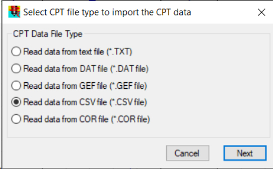
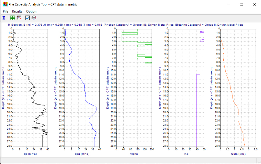
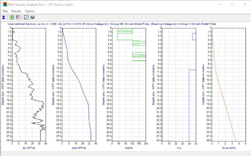
The Innovative Geotechnics ALLCPT program was used for raw CPT processing and axial pile resistance computations using the LCPC method. Only metric units can be imported and reported using the current version of ALLCPT (Version 2.5). Therefore, the unscalped, raw, CPT data that were shown previously in Figure G2 and tabulated in Table G3 were converted from imperial units to metric units and imported into the ALLCPT program using the Data – Add CPT tab in the main window. Specifically, the CPT data that were contained in a .CSV file were imported using the Read data from CSV file (*.CSV file) toggle (Figure G4).

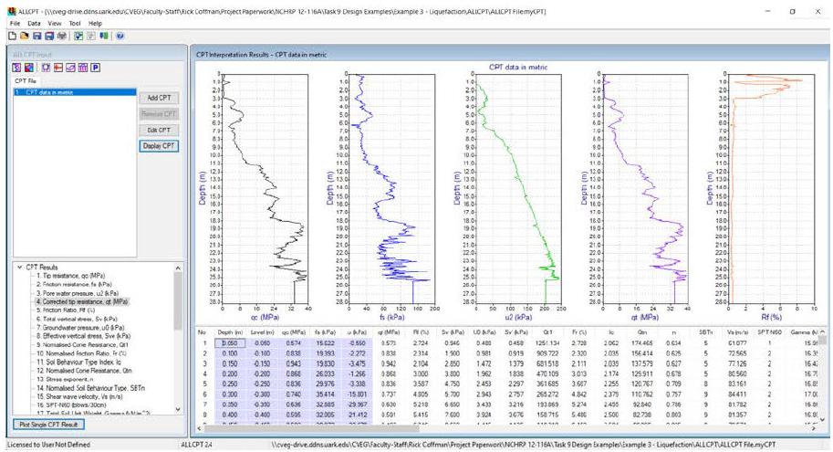
After uploading the data, the predominant CPT parameters (qc, fs, u2, qt, Rf) are graphically displayed in the upper right hand side of the main window (Figure 5). All of the correlated values that were obtained from the ALLCPT calculations are also tabulated in the lower right of the main window. Pop-out windows with graphs for any variable can be obtained by selecting on the variable of interest in the bottom left of the main window.

***Figure G4. Select CPT file type to import the CPT data in ALLCPT.***

Page 175

Suggested Citation: "Appendix G: Design Example 5 - Liquefaction in Sand (H-Pile) Using ALLCPT and TZPILE." National Academies of Sciences, Engineering, and Medicine. 2024. Pile Design for Downdrag: Examples and Supporting Materials. Washington, DC: The National Academies Press. doi: 10.17226/27864.

***Figure G5. ALLCPT main window after importing CPT data.***

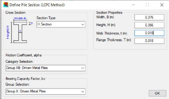
H-pile pile section

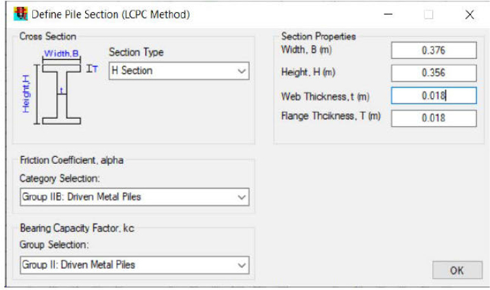
Axial pile resistance computations were performed by selecting Tool – Pile Axial Capacity Tool from the ALLCPT ribbon. The results that were shown in the pop-out window were for the default pile type. To obtain the correct design calculations, the pile information was required. The pile information, including the: cross section, friction coefficient, bearing capacity factor, width, height, web thickness and flange thickness were input into the Define Pile Section (LCPC Method) pop-out window that was obtained by selecting on Pile – Pile Section within the Pile Capacity Analysis Tool (Figure G6). The Options – Advanced Settings feature was used to select the design approach and establish proper factors of safety. A working load design methodology and factors of safety of unity were selected (Figure G7).

***Figure G6. Pile information in the Pile – Pile Section pop out of the Pile Capacity Analysis Tool.***

Page 176

Suggested Citation: "Appendix G: Design Example 5 - Liquefaction in Sand (H-Pile) Using ALLCPT and TZPILE." National Academies of Sciences, Engineering, and Medicine. 2024. Pile Design for Downdrag: Examples and Supporting Materials. Washington, DC: The National Academies Press. doi: 10.17226/27864.

Step 4: Compute the incemental side resistance

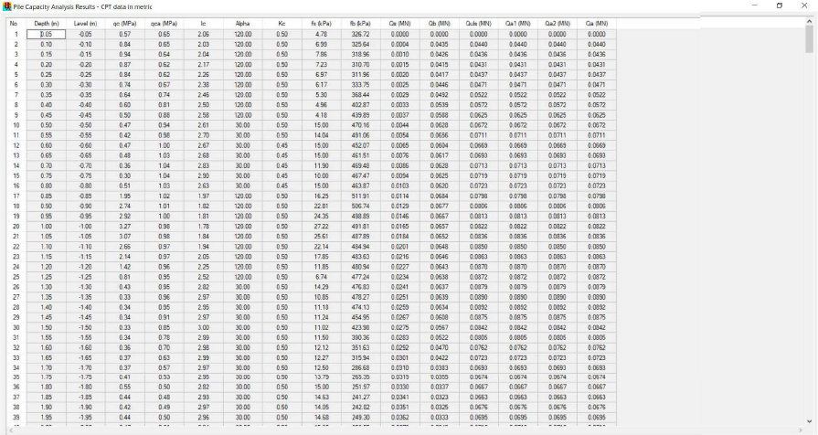
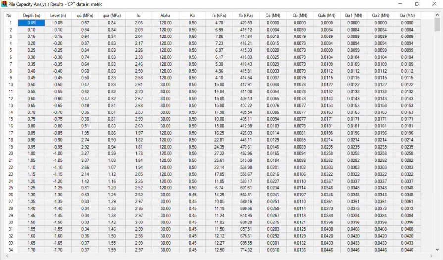
After inputting the correct pile and design information, the desired pile resistance output was obtained (Figure G8). Unlike the FB-Deep program, the LCPC computations from the ALLCPT Pile Capacity Analysis Tool were not limited based on by using weakest values for each soil type. The tabulated values from the Pile Capacity Analysis Tool were obtained by selecting Results – Results Table from the ribbon in the Pile Capacity Analysis Tool window (Figure G9). The results were also exported to a .CSV file for additional processing. The unit side resistance is identified as the fs (kPa) term Results – Results Table shown in Figure G9. These unit side resistance values are also provided in Table G8 for completeness.

***Figure G8. LCPC pile resistance output for the H-pile section.***

Page 177

Suggested Citation: "Appendix G: Design Example 5 - Liquefaction in Sand (H-Pile) Using ALLCPT and TZPILE." National Academies of Sciences, Engineering, and Medicine. 2024. Pile Design for Downdrag: Examples and Supporting Materials. Washington, DC: The National Academies Press. doi: 10.17226/27864.

The ALLCPT output: Depth (m), fs (kPa), fb (kPa), Qs (kN), and Qb (kN) parameters that were shown previously in Figure G9, were exported to Microsoft Excel for additional processing including unit conversion (Table G8, with each variable being defined in the table). The processing required a correction to the ALLCPT Qb data because the ALLCPT program used the gross pile area (0.134m²) in the Qb calculation instead of the pile tip area (0.019m²). The change in side resistance per increment of depth (∆Q), total load in the pile (Q), including the unfactored top load and total resistance (R) in the pile were obtained following calculations that were similar to the calculations used in Design Example 2 and presented herein as Equations 32 through 35. The load, resistance, and combined load and resistance plots obtained from the ALLCPT Pile Capacity Analysis Tool output and additional processing are presented as Figure G10.

***Figure G9. H-Pile section results from the Pile Capacity Analysis Tool by selecting Results – Results Table.***

Q_{i} = (ULS {Qs}_{i}) + U T L

Eqn. 32

Δ Q_{i} = ULS {Qs}_{j} - ULS {Qs}_{i} | j = i + 1 t o j = n

Eqn. 33

R_{b} = f_{b} \cdot A_{t}

Eqn. 34

R_{i} = R_{b} = \sum Δ Q_{i} | i = n t o i = 1

Eqn. 35

Page 178

Suggested Citation: "Appendix G: Design Example 5 - Liquefaction in Sand (H-Pile) Using ALLCPT and TZPILE." National Academies of Sciences, Engineering, and Medicine. 2024. Pile Design for Downdrag: Examples and Supporting Materials. Washington, DC: The National Academies Press. doi: 10.17226/27864.

Table G8. Results from ALLCPT Pile Capacity Analysis and calculations (reported in imperial units).

z	Q_s	Q_b	∆Q_s	Q_wUTL	R	Min(Q,R)	Comments: z=Depth [ft], Q_s=Summation of side resistance from ALLCPT pile capacity analysis [tons], Q_b=End resistance from ALLCPT pile capacity analysis [tons], ∆Q=Incremental side resistance [tons], Q_wUTL=Load in pile with unfactored top load [tons], R=Resistance in pile [tons], Min(Q,R)=Load [tons] used to develop combination curve to identify the location of the neutral plane. Values calculated every ∆z=0.164ft but reported herein every ∆z=0.984ft (except for first and last values).
0.164	0.000	0.000	0.000	107.000	378.116	107.000
1.148	0.326	5.530	0.045	107.326	377.835	107.326
2.133	0.854	6.935	0.124	107.854	377.385	107.854
3.117	1.641	7.497	0.191	108.641	376.666	108.641
4.101	2.630	7.171	0.079	109.630	375.564	109.630
5.085	3.181	5.868	0.090	110.181	375.024	110.181
6.070	3.833	3.631	0.124	110.833	374.406	110.833
7.054	4.564	4.069	0.124	111.564	373.676	111.564
8.038	5.294	5.418	0.124	112.294	372.945	112.294
9.022	6.036	10.094	0.124	113.036	372.203	113.036
10.007	6.789	18.749	0.157	113.789	371.484	113.789
10.991	8.194	26.977	0.225	115.194	370.146	115.194
11.975	9.611	33.778	0.225	116.611	368.730	116.611
12.959	11.139	38.959	0.270	118.139	367.246	118.139
13.944	12.735	45.344	0.281	119.735	365.661	119.735
14.928	14.298	52.763	0.303	121.298	364.121	121.298
15.912	16.456	59.934	0.393	123.456	362.053	123.456
16.896	18.850	62.182	0.393	125.850	359.659	125.850
17.881	21.065	58.462	0.326	128.065	357.377	128.065
18.865	23.077	51.054	0.337	130.077	355.376	130.077
19.849	24.605	42.039	0.247	131.605	353.758	131.605
20.833	26.157	36.498	0.225	133.157	352.184	133.157
21.818	27.494	35.205	0.225	134.494	350.846	134.494
22.802	28.933	36.486	0.292	135.933	349.475	135.933
23.786	30.563	39.162	0.225	137.563	347.778	137.563
24.770	31.968	41.039	0.236	138.968	346.384	138.968
25.755	33.395	42.095	0.236	140.395	344.956	140.395
26.739	34.800	43.624	0.259	141.800	343.574	141.800
27.723	36.205	46.153	0.247	143.205	342.157	143.205
28.707	37.723	49.874	0.270	144.723	340.662	144.723
29.692	39.387	54.617	0.303	146.387	339.033	146.387
30.676	41.275	59.608	0.337	148.275	337.178	148.275
31.660	43.354	64.262	0.348	150.354	335.110	150.354
32.644	45.580	68.724	0.382	152.580	332.918	152.580
33.629	47.862	73.951	0.371	154.862	330.625	154.862
34.613	50.267	82.280	0.416	157.267	328.264	157.267
35.597	52.943	74.783	0.450	159.943	325.623	159.943
36.581	55.888	85.675	0.540	162.888	322.768	162.888
37.566	59.990	96.713	0.731	166.990	318.856	166.990
38.550	64.441	105.143	0.708	171.441	314.382	171.441
39.567	69.039	111.483	0.742	176.039	309.819	176.039
40.551	73.782	116.024	0.821	180.782	305.154	180.782
41.535	78.515	120.824	0.798	185.515	300.399	185.515
42.585	83.865	127.545	0.821	190.865	295.071	190.865
43.570	89.148	133.019	0.910	196.148	289.878	196.148
44.554	94.847	135.526	0.955	201.847	284.224	201.847
45.538	100.849	135.616	0.978	207.849	278.244	207.849
46.522	106.616	134.121	0.899	213.616	272.399	213.616

Page 179

Suggested Citation: "Appendix G: Design Example 5 - Liquefaction in Sand (H-Pile) Using ALLCPT and TZPILE." National Academies of Sciences, Engineering, and Medicine. 2024. Pile Design for Downdrag: Examples and Supporting Materials. Washington, DC: The National Academies Press. doi: 10.17226/27864.

z	Q_s	Q_b	∆Q_s	Q_wUTL	R	Min(Q,R)	Comments: See definition of variables on previous page.
47.507	s 111.719	133.626	s 0.832	218.719	267.229	, 218.719
48.524	116.755	135.919	0.843	223.755	262.204	223.755
49.508	122.431	140.202	0.978	229.431	256.663	229.431
50.492	128.355	143.687	0.989	235.355	250.750	235.355
51.476	134.278	144.091	0.989	241.278	244.826	241.278
52.461	140.135	142.237	0.967	247.135	238.948	238.948
53.445	145.912	139.899	0.944	252.912	233.148	233.148
54.429	151.364	138.606	0.877	258.364	227.629	227.629
55.479	157.220	139.955	0.955	264.220	221.851	221.851
56.463	163.133	143.777	0.989	270.133	215.972	215.972
57.448	168.978	152.364	0.978	275.978	210.116	210.116
58.465	174.991	168.966	0.978	281.991	204.102	204.102
59.449	180.915	185.962	0.989	287.915	198.190	198.190
60.433	186.839	201.328	0.989	293.839	192.266	192.266
61.483	193.088	214.479	0.989	300.088	186.016	186.016
62.467	199.001	218.896	0.978	306.001	180.093	180.093
63.451	204.925	217.424	0.989	311.925	174.180	174.180
64.469	211.006	214.119	0.978	318.006	168.088	168.088
65.518	217.323	207.409	1.383	324.323	162.175	162.175
66.503	223.247	199.833	0.989	330.247	155.858	155.858
67.618	230.002	190.042	0.989	337.002	149.103	149.103
68.602	235.926	181.117	0.989	342.926	143.179	143.179
69.587	241.838	174.148	0.978	348.838	137.255	137.255
70.571	247.762	167.809	0.989	354.762	131.343	131.343
71.555	253.686	165.066	0.989	360.686	125.419	125.419
72.539	259.598	167.033	0.978	366.598	119.495	119.495
73.720	266.590	175.486	0.989	373.590	112.515	112.515
74.705	272.513	182.140	0.989	379.513	106.591	106.591
75.689	278.426	185.614	0.978	385.426	100.668	100.668
77.001	286.485	187.828	0.989	393.485	92.619	92.619
77.986	292.330	190.481	0.989	399.330	86.774	86.774
78.970	298.254	198.034	0.989	405.254	80.851	80.851
79.987	304.178	206.712	0.989	411.178	74.927	74.927
80.971	310.090	213.748	0.989	417.090	69.015	69.015
81.923	316.014	216.120	0.989	423.014	63.091	63.091
82.907	321.938	213.692	0.989	428.938	57.167	57.167
83.825	327.356	209.612	0.978	434.356	51.738	51.738
84.810	333.279	205.846	0.989	440.279	45.826	45.826
85.794	339.192	203.531	0.978	446.192	39.902	39.902
86.778	345.115	202.418	0.989	452.115	33.989	33.989
87.434	349.061	202.384	0.989	456.061	30.044	30.044

Page 180

Suggested Citation: "Appendix G: Design Example 5 - Liquefaction in Sand (H-Pile) Using ALLCPT and TZPILE." National Academies of Sciences, Engineering, and Medicine. 2024. Pile Design for Downdrag: Examples and Supporting Materials. Washington, DC: The National Academies Press. doi: 10.17226/27864.

Step 5: Develop a depth-dependent load profile

The depth-dependent load in the pile is reported in Table G8. Specifically, the Q_wUTL term that represents the load in pile with the unfactored top load in units of tons is the term of interest. A standalone plot of the Q_wUTL term as a function of depth can be generated to observe how the load develops as a function of depth. However, this plot has been included as the “Load” curve in Figure G10.

Step 6: Calculate the end bearing resistance; develop the depth-dependent resistance profile

The end bearing resistance and the depth-dependent resistance profile are also included in Table G8. The end bearing resistance was taken as the Qb value at a depth of 26.65m (87.43ft); a depth of 26.65m was the closest depth to the actual length of the pile (26.67m=87.5ft). A end bearing resistance of 30.04 tons was obtained after using the aforementioned pile tip area 0.019m² instead of the gross pile area 0.134m².

***Figure G10. H-pile predicted neutral plane based on ALLCPT Pile Capacity Analysis Tool output with additional processing. Note: converted to imperial units.***

The depth-dependent resistance in the pile (R) is reported in Table G8. A standalone plot of the R term as a function of depth can be generated to observe how the resistance develops as a function of depth. However, this plot has been included as the “Resistance” curve in Figure G10.

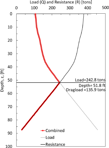
Step 7: Develop the depth-dependent combined load-resistance curve

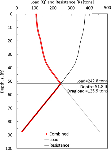
The combined load-resistance curve is also presented in Figure G10. This curve was obtained by selecting the minimum value of load and resistance at each given depth. The depth-dependent values of the combined load-resistance curve are presented in the Min(Q,R) column in Table G8.

Step 8: Identify the location of the neutral plane from the combined load-resistance curve

As shown previously in Figure G10, the neutral plane was identified at a depth of 51.8ft. This depth corresponded with the intersection of the “Load’ and “Resistance” curves that were developed in Steps 5 and 6, respectively. The depth also corresponded with the largest load observed for the depth depended combined load-resistance curve.

Step 9: Calculate the amount of drag load in the pile

From the depth-dependent combined load-resistance curve (Figure G10), the maximum load was 282.8 tons. This load results in an observed drag load of 135.9 tons. As expected, the drag load was observed to be the largest at the location of the neutral plane.

Page 181

Suggested Citation: "Appendix G: Design Example 5 - Liquefaction in Sand (H-Pile) Using ALLCPT and TZPILE." National Academies of Sciences, Engineering, and Medicine. 2024. Pile Design for Downdrag: Examples and Supporting Materials. Washington, DC: The National Academies Press. doi: 10.17226/27864.

Step 10: Calculate the toe settlement and elastic compression in the pile

A settlement analysis was also performed using the Fleming (1992) approach. Key parameters for the Fleming approach were input into the Pile Capacity Analysis Option pop-out window obtained by selecting Option – Advanced Setting within the Pile Capacity Analysis Tool window. The values that were used for the advanced settings are presented in Figure G7 (the same figure that was referenced previously for input of the design approach). The value for the soil stiffness at the pile base, Eb (kPa) parameter, that is shown in Figure G7 was obtained from row 527 of the Es (MPa) column of the table shown in the bottom right corner of Figure G5 (Es=148.714 Mpa). This row corresponded with the depth of the pile tip. The pile settlement graph (Figure G11) was then obtained by selecting on the Pile Settlement Analysis tab in the Pile Capacity Analysis Tool ribbon after the Pile Capacity Analysis Option window was closed. The values were exported to Microsoft Excel after selecting on Display Results >>.

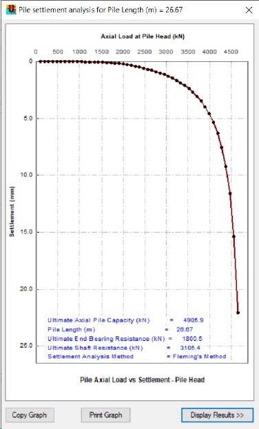
***Figure G11. H-pile section pile settlement analysis graph. Gross end area used.***

The aforementioned limitation associated with the ALLCPT program of using the pile gross area instead of the pile tip adversely impacts the pile settlement curve. Unlike the ALLCPT output (depth, fs, fb, Qs, and Qb) where the data can be manipulated to correct for the use of the incorrect area, the use of the wrong area cannot be corrected in the load-settlement curve. Innovative Geotechnics, the creators of the software, have suggested use of the User Defined pile section rather than the H-pile pile section until the next release of the software enables either gross area or tip area to be considered.

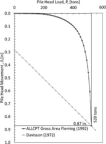
The Davisson (1972) method was used in conjunction with the settlement curve presented in Figure G11 to determine the pile tip movement. This pile tip movement was used in association with the elastic compression data to determine the predicted location of the neutral plane using a soil settlement-pile settlement plot. The pile head settlement was obtained by using the Davisson (1972) method along with the developed Fleming (1992) curve.

Step 11: Calculate the geotechnical resistance of the pile

The geotechnical resistance was also obtained by using the Davisson (1972) method along with the developed Fleming (1992) curve. Specifically, the pile head load value obtained from the intersection of the Davisson (1972) curve and the Fleming (1992) curve was the geotechnical resistance. The observed

Page 182

Suggested Citation: "Appendix G: Design Example 5 - Liquefaction in Sand (H-Pile) Using ALLCPT and TZPILE." National Academies of Sciences, Engineering, and Medicine. 2024. Pile Design for Downdrag: Examples and Supporting Materials. Washington, DC: The National Academies Press. doi: 10.17226/27864.

geotechnical resistance of the pile was 520 tons. However, it must be noted that this resistance was obtained by using the gross area pile instead of the end area of the pile.

Step 12: Identify the location and the settlement of the neutral plane (from the soil settlement-pile settlement curve)

The elastic compression in the pile was also computed (Equations 30 and 31 as previously presented). The cumulative elastic compression was subtracted from the pile head movement (determined in Step 11), as a function of depth, to determine the amount of settlement of the pile. As shown in Figure G13, the pile head settled by 0.870in and the pile toe settled by 0.533in. The soil settlement shown in Figure G13 was obtained previously in Step 2. From the soil settlement-pile settlement curve, the neutral plane was observed to occur at a depth of 24.9ft. The settlement of the neutral plane was 0.789in.

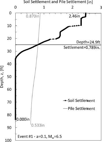
***Figure G12. H-pile load-settlement curve. Note: use of gross end area instead of pile tip area.***

Figure G13. H-pile predicted neutral plane location from the pile settlement and soil settlement as based on ALLCPT Pile Capacity Analysis Tool output with additional processing. Note: use of gross end area instead of pile tip area.

The location of the neutral plane (51.8ft) that was determined from the load-resistance curve was not within 5 feet of the location of the neutral plane (24.9ft) that was determined from the soil settlement-pile settlement curve. The use of the gross cross-sectional area instead of the pile tip area may have contributed to the difference in the locations of the neutral plane. The size of the pile (length and diameter) and type of pile (elastic compression) may have also contributed to the difference in the

Page 183

Suggested Citation: "Appendix G: Design Example 5 - Liquefaction in Sand (H-Pile) Using ALLCPT and TZPILE." National Academies of Sciences, Engineering, and Medicine. 2024. Pile Design for Downdrag: Examples and Supporting Materials. Washington, DC: The National Academies Press. doi: 10.17226/27864.

locations of the neutral planes. Moreover, the fully-mobilized conditions may not be reached resulting in a need to perform and analysis on partially-mobilized conditions.

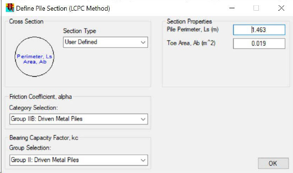
“User Defined” pile section

When using the User Defined selection within the Pile–Pile Section pop-out of the Pile Capacity Analysis Tool, the pile perimeter and toe area are required inputs (Figure G14). An equivalent H-pile selection that only considered the tip area rather than the gross area for the bearing capacity calculations was created. The Pile Perimeter was set to 1.436m, and the Toe Area was set to 0.019m².

***Figure G14. User Defined pile information in the Pile – Pile Section pop out window of the Pile Capacity Analysis Tool.***

The working load design methodology and factors of safety of unity that were previously selected for the H-pile case (as shown previously Figure G6) were also used for the user defined case. After the correct pile and design information was input, the desired pile resistance output was obtained (Figure G15). The tabulated values from the Pile Capacity Analysis Tool were obtained by selecting Results – Results Table from the ribbon in the Pile Capacity Analysis Tool window (Figure G16). The results were also exported to a .CSV file for additional processing.

Page 184

Suggested Citation: "Appendix G: Design Example 5 - Liquefaction in Sand (H-Pile) Using ALLCPT and TZPILE." National Academies of Sciences, Engineering, and Medicine. 2024. Pile Design for Downdrag: Examples and Supporting Materials. Washington, DC: The National Academies Press. doi: 10.17226/27864.

***Figure G15. LCPC pile resistance output for the H-pile equivalent User Defined pile section.***

***Figure G16. User Defined pile section results from the Pile Capacity Analysis Tool.***

Page 185

Suggested Citation: "Appendix G: Design Example 5 - Liquefaction in Sand (H-Pile) Using ALLCPT and TZPILE." National Academies of Sciences, Engineering, and Medicine. 2024. Pile Design for Downdrag: Examples and Supporting Materials. Washington, DC: The National Academies Press. doi: 10.17226/27864.

The ALLCPT output: Depth (m), fs (kPa), fb (kPa), Qs (kN), and Qb (kN) parameters that were shown previously in Figure G16, were exported to Microsoft Excel for additional processing including unit conversion (Table G9, with each variable being defined in the table). Like with the H-pile pile section, a neutral plane location was determined as the intersection of the load and resistance curves developed from the processed data for the user defined pile section. The load within the pile, as a function of depth, is presented in Figure G17.

***Figure G17. Predicted neutral plane based on ALLCPT Pile Capacity Analysis Tool output with additional processing for User Defined pile section. Note: converted to imperial units.***

The pile settlement graph (Figure G18) was obtained by selecting on the Pile Settlement Analysis tab in the Pile Capacity Analysis Tool ribbon after the Pile Capacity Analysis Option window was closed. The values were exported to Microsoft Excel after selecting on Display Results >>. The Davisson (1972) method was used in conjunction with the pile settlement curve (Figure G19) to determine the pile tip movement. This pile tip movement was used in association with the elastic compression data to determine the predicted location of the neutral plane via the soil settlement-pile settlement plot. By combining the pile settlement analysis and the soil settlement analysis, the neutral plane was predicted to occur at a depth of 28.0ft (Figure G20).

Page 186

Suggested Citation: "Appendix G: Design Example 5 - Liquefaction in Sand (H-Pile) Using ALLCPT and TZPILE." National Academies of Sciences, Engineering, and Medicine. 2024. Pile Design for Downdrag: Examples and Supporting Materials. Washington, DC: The National Academies Press. doi: 10.17226/27864.

***Figure G18. User Defined pile section pile settlement analysis graph.***

User Defined pile section pile settlement analysis graph withDavisson (1972) Note: converted to imperial units — ***Figure G19. User Defined pile section pile settlement analysis graph with Davisson (1972). Note: converted to imperial units.***

***Figure G20. User Defined pile settlement and soil settlement as a function of depth.***

Page 187

Suggested Citation: "Appendix G: Design Example 5 - Liquefaction in Sand (H-Pile) Using ALLCPT and TZPILE." National Academies of Sciences, Engineering, and Medicine. 2024. Pile Design for Downdrag: Examples and Supporting Materials. Washington, DC: The National Academies Press. doi: 10.17226/27864.

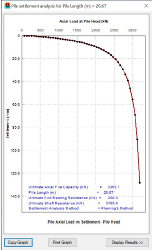
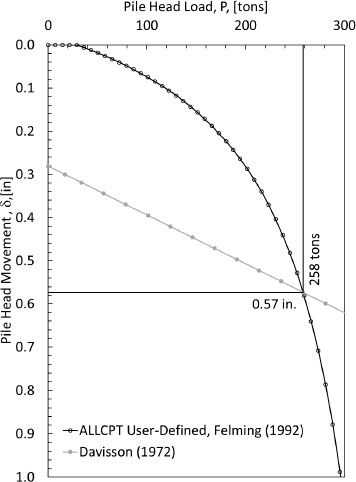
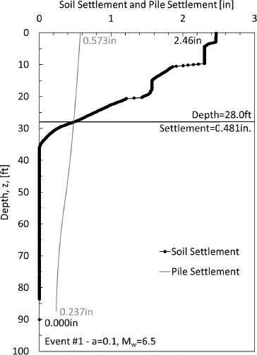
Table G9. Results from ALLCPT Pile Capacity Analysis and calculations (reported in imperial units).

z	Q_s	Qb	∆Q_s	Q_wUTL	R	Min(Q,R)	Comments: z=Depth [ft], Q_s=Summation of side resistance from ALLCPT pile capacity analysis [tons], Q_b=End resistance from ALLCPT pile capacity analysis [tons], ∆Q=Incremental side resistance [tons], Q_wUTL=Load in pile with unfactored top load [tons], R=Resistance in pile [tons], Min(Q,R)=Load [tons] used to develop combination curve to identify the location of the neutral plane. Values calculated every ∆z=0.164ft but reported herein every ∆z=0.984ft (except for first and last values). See definition of variables on previous page.
0.164	0.000	0.000	0.000	107.000	378.116	107.000
1.148	0.326	5.530	0.045	107.326	377.835	107.326
2.133	0.854	6.935	0.124	107.854	377.385	107.854
3.117	1.641	7.497	0.191	108.641	376.666	108.641
4.101	2.630	7.171	0.079	109.630	375.564	109.630
5.085	3.181	5.868	0.090	110.181	375.024	110.181
6.070	3.833	3.631	0.124	110.833	374.406	110.833
7.054	4.564	4.069	0.124	111.564	373.676	111.564
8.038	5.294	5.418	0.124	112.294	372.945	112.294
9.022	6.036	10.094	0.124	113.036	372.203	113.036
10.007	6.789	18.749	0.157	113.789	371.484	113.789
10.991	8.194	26.977	0.225	115.194	370.146	115.194
11.975	9.611	33.778	0.225	116.611	368.730	116.611
12.959	11.139	38.959	0.270	118.139	367.246	118.139
13.944	12.735	45.344	0.281	119.735	365.661	119.735
14.928	14.298	52.763	0.303	121.298	364.121	121.298
15.912	16.456	59.934	0.393	123.456	362.053	123.456
16.896	18.850	62.182	0.393	125.850	359.659	125.850
17.881	21.065	58.462	0.326	128.065	357.377	128.065
18.865	23.077	51.054	0.337	130.077	355.376	130.077
19.849	24.605	42.039	0.247	131.605	353.758	131.605
20.833	26.157	36.498	0.225	133.157	352.184	133.157
21.818	27.494	35.205	0.225	134.494	350.846	134.494
22.802	28.933	36.486	0.292	135.933	349.475	135.933
23.786	30.563	39.162	0.225	137.563	347.778	137.563
24.770	31.968	41.039	0.236	138.968	346.384	138.968
25.755	33.395	42.095	0.236	140.395	344.956	140.395
26.739	34.800	43.624	0.259	141.800	343.574	141.800
27.723	36.205	46.153	0.247	143.205	342.157	143.205
28.707	37.723	49.874	0.270	144.723	340.662	144.723
29.692	39.387	54.617	0.303	146.387	339.033	146.387
30.676	41.275	59.608	0.337	148.275	337.178	148.275
31.660	43.354	64.262	0.348	150.354	335.110	150.354
32.644	45.580	68.724	0.382	152.580	332.918	152.580
33.629	47.862	73.951	0.371	154.862	330.625	154.862
34.613	50.267	82.280	0.416	157.267	328.264	157.267
35.597	52.943	74.783	0.450	159.943	325.623	159.943
36.581	55.888	85.675	0.540	162.888	322.768	162.888
37.566	59.990	96.713	0.731	166.990	318.856	166.990
38.550	64.441	105.143	0.708	171.441	314.382	171.441
39.567	69.039	111.483	0.742	176.039	309.819	176.039
40.551	73.782	116.024	0.821	180.782	305.154	180.782
41.535	78.515	120.824	0.798	185.515	300.399	185.515
42.585	83.865	127.545	0.821	190.865	295.071	190.865
43.570	89.148	133.019	0.910	196.148	289.878	196.148
44.554	94.847	135.526	0.955	201.847	284.224	201.847
45.538	100.849	135.616	0.978	207.849	278.244	207.849
46.522	106.616	134.121	0.899	213.616	272.399	213.616

Page 188

Suggested Citation: "Appendix G: Design Example 5 - Liquefaction in Sand (H-Pile) Using ALLCPT and TZPILE." National Academies of Sciences, Engineering, and Medicine. 2024. Pile Design for Downdrag: Examples and Supporting Materials. Washington, DC: The National Academies Press. doi: 10.17226/27864.

z	Q_s	Qb	∆Q_s	Q_wUTL	R	Min(Q,R)	Comments: z=Depth [ft], Q_s=Summation of side resistance from ALLCPT pile capacity analysis [tons], Q_b=End resistance from ALLCPT pile capacity analysis [tons], ∆Q=Incremental side resistance [tons], Q_wUTL=Load in pile with unfactored top load [tons], R=Resistance in pile [tons], Min(Q,R)=Load [tons] used to develop combination curve to identify the location of the neutral plane. Values calculated every ∆z=0.164ft but reported herein every ∆z=0.984ft (except for first and last values). See definition of variables on previous page.
47.507	111.719	133.626	0.832	218.719	267.229	218.719
48.524	116.755	135.919	0.843	223.755	262.204	223.755
49.508	122.431	140.202	0.978	229.431	256.663	229.431
50.492	128.355	143.687	0.989	235.355	250.750	235.355
51.476	134.278	144.091	0.989	241.278	244.826	241.278
52.461	140.135	142.237	0.967	247.135	238.948	238.948
53.445	145.912	139.899	0.944	252.912	233.148	233.148
54.429	151.364	138.606	0.877	258.364	227.629	227.629
55.479	157.220	139.955	0.955	264.220	221.851	221.851
56.463	163.133	143.777	0.989	270.133	215.972	215.972
57.448	168.978	152.364	0.978	275.978	210.116	210.116
58.465	174.991	168.966	0.978	281.991	204.102	204.102
59.449	180.915	185.962	0.989	287.915	198.190	198.190
60.433	186.839	201.328	0.989	293.839	192.266	192.266
61.483	193.088	214.479	0.989	300.088	186.016	186.016
62.467	199.001	218.896	0.978	306.001	180.093	180.093
63.451	204.925	217.424	0.989	311.925	174.180	174.180
64.469	211.006	214.119	0.978	318.006	168.088	168.088
65.518	217.323	207.409	1.383	324.323	162.175	162.175
66.503	223.247	199.833	0.989	330.247	155.858	155.858
67.618	230.002	190.042	0.989	337.002	149.103	149.103
68.602	235.926	181.117	0.989	342.926	143.179	143.179
69.587	241.838	174.148	0.978	348.838	137.255	137.255
70.571	247.762	167.809	0.989	354.762	131.343	131.343
71.555	253.686	165.066	0.989	360.686	125.419	125.419
72.539	259.598	167.033	0.978	366.598	119.495	119.495
73.720	266.590	175.486	0.989	373.590	112.515	112.515
74.705	272.513	182.140	0.989	379.513	106.591	106.591
75.689	278.426	185.614	0.978	385.426	100.668	100.668
77.001	286.485	187.828	0.989	393.485	92.619	92.619
77.986	292.330	190.481	0.989	399.330	86.774	86.774
78.970	298.254	198.034	0.989	405.254	80.851	80.851
79.987	304.178	206.712	0.989	411.178	74.927	74.927
80.971	310.090	213.748	0.989	417.090	69.015	69.015
81.923	316.014	216.120	0.989	423.014	63.091	63.091
82.907	321.938	213.692	0.989	428.938	57.167	57.167
83.825	327.356	209.612	0.978	434.356	51.738	51.738
84.810	333.279	205.846	0.989	440.279	45.826	45.826
85.794	339.192	203.531	0.978	446.192	39.902	39.902
87.434	349.061	202.384	0.989	456.061	30.044	30.044

Neutral plane location determination using Ensoft TZPILE with User Defined ALLCPT data as input

Because the difference in the neutral plane locations (23.8ft) was much greater than required difference (5ft), the User Defined ALLCPT data were used as input into the Ensoft TZPILE program. This is a modified version of Method B approach recommended by the NCHRP12-116A project team, in which previously collected Method A data is used as an input. Each of the input screens from the TZPILE

Page 189

Suggested Citation: "Appendix G: Design Example 5 - Liquefaction in Sand (H-Pile) Using ALLCPT and TZPILE." National Academies of Sciences, Engineering, and Medicine. 2024. Pile Design for Downdrag: Examples and Supporting Materials. Washington, DC: The National Academies Press. doi: 10.17226/27864.

program, with each containing information for this design example, are included as Figures G21–G24. The pile properties are included as Figure G21. The AE properties are included as Figure G22. The soil properties are included as Figure G23. The soil settlement properties are included as Figure G24. The output from the program included load in the pile and pile settlement. The load in the pile as a function of depth is presented in Figure G25. The pile settlement and soil settlement are presented in Figure G26. The location of the neutral plane from the ALLCPT-TZPILE output (32.3ft) was in close agreement with the CAPWAP prediction (33.6ft). The data from Figures G25 and G26 are presented in Table G10.

***Figure G21. Pile properties in TZPILE.***

***Figure G22. AE properties in TZPILE.***

Page 190

Suggested Citation: "Appendix G: Design Example 5 - Liquefaction in Sand (H-Pile) Using ALLCPT and TZPILE." National Academies of Sciences, Engineering, and Medicine. 2024. Pile Design for Downdrag: Examples and Supporting Materials. Washington, DC: The National Academies Press. doi: 10.17226/27864.

***Figure G23. Soil properties in TZPILE.***

***Figure G24. Soil settlement properties in TZPILE.***

Page 191

Suggested Citation: "Appendix G: Design Example 5 - Liquefaction in Sand (H-Pile) Using ALLCPT and TZPILE." National Academies of Sciences, Engineering, and Medicine. 2024. Pile Design for Downdrag: Examples and Supporting Materials. Washington, DC: The National Academies Press. doi: 10.17226/27864.

***Figure G25. Comparison of TZPILE using ALLCPT.***

***Figure G26. Settlement from TZPILE using ALLCPT.***

Page 192

Suggested Citation: "Appendix G: Design Example 5 - Liquefaction in Sand (H-Pile) Using ALLCPT and TZPILE." National Academies of Sciences, Engineering, and Medicine. 2024. Pile Design for Downdrag: Examples and Supporting Materials. Washington, DC: The National Academies Press. doi: 10.17226/27864.

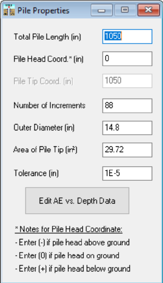
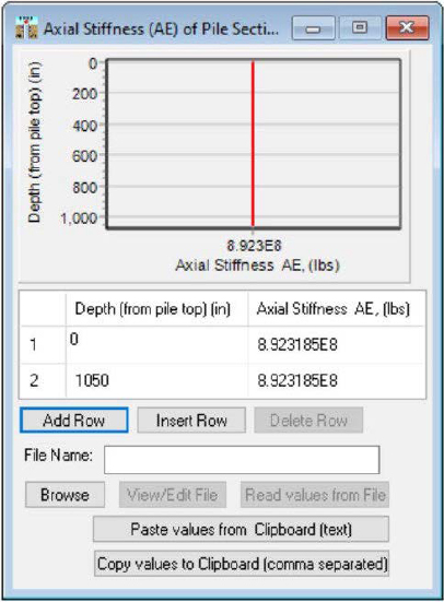
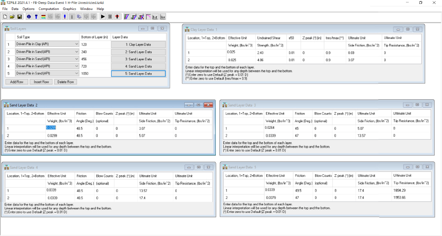
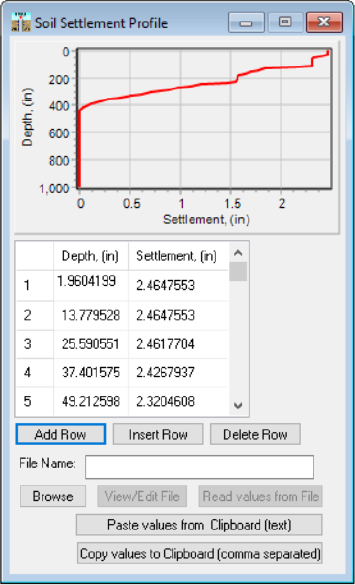
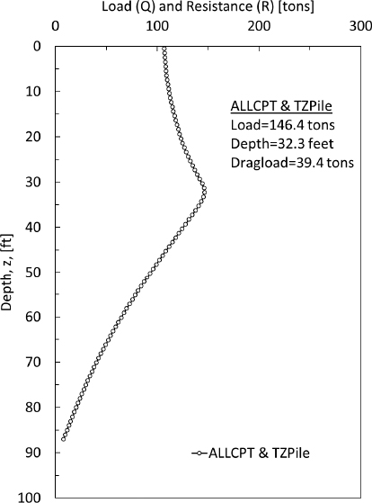
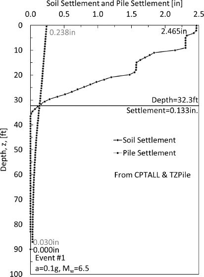
Table G10. Results from ALLCPT/TZPILE and additional spreadsheet calculations.

z	Min(Q,R)	p	Comments:z=Depth [ft], Min(Q,R)=Load used to develop combination curve to identify the location of the neutral plane, p =pile settlement.
0.5	106.95	0.238
1.5	107.20	0.235
2.5	107.50	0.232
3.5	107.85	0.229
4.5	108.25	0.226
5.5	108.70	0.223
6.5	109.25	0.220
7.5	109.80	0.217
8.5	110.45	0.215
9.5	111.15	0.212
10.4	111.95	0.209
11.4	112.90	0.206
12.4	113.85	0.203
13.4	114.85	0.199
14.4	115.90	0.196
15.4	117.05	0.193
16.4	118.20	0.190
17.4	119.45	0.187
18.4	120.75	0.184
19.4	122.10	0.181
20.4	123.50	0.177
21.4	125.05	0.174
22.4	126.70	0.171
23.4	128.45	0.167
24.4	130.40	0.164
25.4	132.40	0.160
26.4	134.60	0.157
27.3	136.90	0.153
28.3	139.35	0.149
29.3	141.90	0.146
30.3	144.30	0.142
31.3	146.00	0.138
32.3	146.40	0.134
33.3	145.35	0.130
34.3	143.30	0.126
35.3	140.65	0.122
36.3	137.60	0.119
37.3	134.40	0.115
38.3	131.15	0.111
39.3	127.85	0.108
40.3	124.60	0.105
41.3	121.35	0.101
42.3	118.15	0.098
43.3	114.95	0.095
44.3	111.75	0.092
45.2	108.55	0.089
46.2	105.40	0.086
47.2	102.25	0.083
48.2	99.15	0.081
49.2	96.10	0.078
50.2	93.05	0.075
51.2	90.05	0.073
52.2	87.10	0.071
53.2	84.20	0.068

Page 193

Suggested Citation: "Appendix G: Design Example 5 - Liquefaction in Sand (H-Pile) Using ALLCPT and TZPILE." National Academies of Sciences, Engineering, and Medicine. 2024. Pile Design for Downdrag: Examples and Supporting Materials. Washington, DC: The National Academies Press. doi: 10.17226/27864.

z	Min(Q,R)	δ_p	Comments: See definition of variables on previous page.
55.2	78.45	0.064
56.2	75.60	0.062
57.2	72.85	0.060
58.2	70.05	0.058
59.2	67.35	0.056
60.2	64.65	0.054
61.2	62.00	0.053
62.1	59.40	0.051
63.1	56.85	0.050
64.1	54.30	0.048
65.1	51.85	0.047
66.1	49.45	0.045
67.1	47.09	0.044
68.1	44.79	0.043
69.1	42.53	0.042
70.1	40.33	0.041
71.1	38.17	0.039
72.1	36.06	0.038
73.1	33.99	0.038
74.1	31.96	0.037
75.1	29.96	0.036
76.1	28.00	0.035
77.1	26.08	0.034
78.1	24.18	0.034
79.1	22.31	0.033
80.0	20.47	0.032
81.0	18.65	0.032
82.0	16.85	0.031
83.0	15.08	0.031
84.0	13.32	0.031
85.0	11.57	0.030
86.0	9.84	0.030
87.0	8.12	0.030

Page 194

Suggested Citation: "Appendix G: Design Example 5 - Liquefaction in Sand (H-Pile) Using ALLCPT and TZPILE." National Academies of Sciences, Engineering, and Medicine. 2024. Pile Design for Downdrag: Examples and Supporting Materials. Washington, DC: The National Academies Press. doi: 10.17226/27864.

Conclusion:

A design example related to liquefaction was presented herein. The design example included the use of CPT data and detailed calculations for determining: 1) post-liquefaction reconsolidation settlement within the soil deposit, 2) the location of the neutral plane, 3) the amount of drag load within the pile, and 4) the amount of downdrag expected. The Boulanger and Idriss (2014) CPT-based liquefaction-triggering method, coupled with the Yoshimine et al. (2006) post-liquefaction settlement estimation were used for determination of the post-liquefaction reconsolidation settlement. The Bustamante and Gianeselli (1982) LCPC method was used for determining the load in the pile, as a function of depth. Software programs including ALLCPT (Innovative Geotechnics, 2023a) and TZPILE (Ensoft, 2021) facilitated the LCPC and t-z calculations.

The ALLCPT program allowed for determination of all soil properties developed from correlations with CPT data. The correlated soil properties were then used in the ALLCPT program to determine axial resistance estimates. Although only one pile size was considered, the axial resistance estimates can be determined for various pile shapes and sizes. Moreover, a load-settlement curve was generated using the ALLCPT program based on the Fleming (1992) approach. The pile head movement from the developed load-settlement curve, the load in the pile from the axial resistance estimate, and the soil settlement data from the post-liquefaction reconsolidation settlement were used to develop the soil settlement-pile settlement curve for determination of the neutral plane. Using the data from the ALLCPT program, the locations of the neutral plane that were determined from the load-resistance curve and from the soil settlement-pile settlement curve were significantly different (23.8 feet).

The output data from the ALLCPT program were used as input data in the TZPILE program. The TZPILE program allowed for the investigation of differential movement between the pile and the soil. The obtained location of the neutral plane (32.3 feet), drag load (39.4 tons), and downdrag (0.133 inches) that were obtained from the ALLCPT/TZPILE combination were the most representative.

Page 195

Suggested Citation: "Appendix G: Design Example 5 - Liquefaction in Sand (H-Pile) Using ALLCPT and TZPILE." National Academies of Sciences, Engineering, and Medicine. 2024. Pile Design for Downdrag: Examples and Supporting Materials. Washington, DC: The National Academies Press. doi: 10.17226/27864.

References

Andrus, R.D., Hayati, H., and Mohanan, N.P. (2009). “Correcting liquefaction resistance for aged sands using measured to estimated velocity ratio.” Journal of Geotechnical and Geoenvironmental Engineering, 135(6): 735–744.

Bong, T. and Stuedlein, A.W. (2018). “Effect of Cone Penetration Conditioning on Random Field Model Parameters and Impact of Spatial Variability on Liquefaction-induced Differential Settlements.” Journal of Geotechnical and Geoenvironmental Engineering, 144(5): 04018018.

Boulanger, R.W. and Idriss, I.M. (2014). “CPT and SPT based liquefaction triggering procedures.” Report No. UCD/CGM.-14, University of California, Davis, California.

Briaud, J-L, Tucker, L.M., Anderson, J.S., Perdomo, D. and Coyle, H.M. (1986). Development of An improved Design Procedure for Single Piles in Clays and Sands, Report No. MSHDRD-86-050-1, Mississippi State Highway Department, Jackson, MS, p. 192.

Bustamante, M., and Gianeselli, L. (1982). Pile bearing capacity predictions by means of static penetrometer CPT, Proceedings of the 2nd European Symposium on Penetration Testing, ESOPT II, Amsterdam, May 24–27, 1982. A.A. Balkema, Rotterdam, Vol. 2, 493–500.

Coffman, R.A., Ishimwe, E. (2018). Evaluating the Capacity of Deep Soils Foundations Final Report for TRC Project 1502. Client: Arkansas State Highway and Transportation Department, March.

Cary, J.R., Stuedlein, A.W., McGann, C.R., Bradley, B.A., and Maurer, B.W. (2022). “Effect of Refinements to CPT-Based Liquefaction Triggering Analysis on Liquefaction Severity Indices at the Avondale Playground Site, Christchurch, NZ.” Proceedings, PBDIV, Fourth Conference on Performance-based Design in Earthquake Geotechnical Engineering, Beijing, China, Springer,1454-1466.

Davisson, M.T. (1972) “High Capacity Piles” Proceedings, Lecture Series, Innovations in Foundation Construction, ASCE, Illinois Section, 52 pp.

Dadashiserej, A., Jana, A., Ortiz, S.C., Walters, J.J., Stuedlein, A.W., and Evans, T.M. (2022). “Monotonic, Cyclic, and Post-Cyclic Response of Willamette River Silt at the Van Buren Bridge.” Proceedings, Geo-Congress 2022: 431–443.

DeCock, F.A. (2009). “Sense and Sensitivity of Pile Load-Deformation Behavior.” Deep Foundation on Board and Auger Piles. Taylor and Francis. 22 pp.

Duku, P.M., Stewart, J.P., Whang, D.H., and Yee, E. (2008). “Volumetric Strains of Clean Sands Subject to Cyclic Loads.” Journal of Geotechnical and Geoenvironmental Engineering, 134(8), 1073-1085.

Ensoft (2021). “TZPILE 2021 v4” TPile Computer Program. Austin, TX

Fleming, W.G.K., (1992). “A New Method For Single Pile Settlement Prediction and Analysis.” Geotechnique, Vol. 42 (3): 411–425.

Hossain, A.M., Andrus, R.D., and Camp III, W.M. (2013). “Correcting Liquefaction Resistance Of Unsaturated Soil Using Wave Velocity.” Journal of Geotechnical and Geoenvironmental Engineering, 139(2), 277-287.

Idriss, I.M., and Boulanger, R.W. (2008). “Soil Liquefaction During Earthquakes.” Monograph MNO-12, Earthquake Engineering Research Institute, Oakland, CA, 261 pp.

Innovative Geotechnics (2023a). “CPT Data Interpretation Tool for Geotechnical Engineering.” ALLCPT 2.5 computer program. Perth, Western Australia.

Page 196

Suggested Citation: "Appendix G: Design Example 5 - Liquefaction in Sand (H-Pile) Using ALLCPT and TZPILE." National Academies of Sciences, Engineering, and Medicine. 2024. Pile Design for Downdrag: Examples and Supporting Materials. Washington, DC: The National Academies Press. doi: 10.17226/27864.

Innovative Geotechnics (2023b). “A Program for Single Piles under Axial Loading.” PileAXL 2.5 computer program. Perth, Western Australia.

Ishihara, K., and Yoshimine, M. (1992). “Evaluation of Settlements in Sand Deposits Following Liquefaction During Earthquakes.” Soils and Foundations, 32(1), 173-188.

Ishimwe, E., Coffman, R.A., Rollins, K.M., (2018). “Analysis of Post-Liquefaction Axial Capacities of Driven Pile and Drilled Shaft Foundations,” Proceedings of ASCE Geo-Institute International Foundations Conference and Equipment Expo. Orlando, FL, March 5-10, 2018.

Jana, A. and Stuedlein, A.W. (2021). “Monotonic, Cyclic, and Post-Cyclic Responses of an Alluvial Plastic Silt Deposit.” Journal of Geotechnical and Geoenvironmental Engineering, 147(3): 04020174.

Lee, K.L. and Albaisa, A. (1974). “Earthquake-Induced Settlements in Saturated Sands.” Journal of the Geotechnical Engineering Division, 100(4), 387-406.

Robertson, P.K., and Cabal, K.L. (2015). Guide to Cone Penetration Testing for Geotechnical Engineering, 6th ed. Gregg Drilling & Testing, Inc.

Rollins, K.M., Miller, N.P., and Hemenway, D. (1999). “Evaluation of Pile Capacity Prediction Methods Based on Cone Penetration Testing Using Results from I-15 Load Tests.” Transportation Research Record 1675, Paper No. 99-0198. pp. 40-50.

Seed, H.B., and Idriss, I.M. (1971). “Simplified Procedure for Evaluating Soil Liquefaction Potential.” Journal of the Soil Mechanics and Foundations Division, 97(9), 1249-1273.

Silvey, A. (2018). “Evaluation and Development of CPT Based Pile Design in Nebraska Soils.” Masters Thesis, University of Nebraska – Lincoln. August.

Stewart, J.P., Smith, P.M., and Whang, D.H. (2002). “Documentation and analysis of field case histories of seismic compression during the 1994 Northridge, California earthquake.” Report No. PEER 2002/09, Pacific Earthquake Engineering Research Center, University of California, Berkeley, California, 246 pp.

Stuedlein, A.W., Alemu, B., Evans, T.M., Kramer, S.L., Stewart, J.P., Ulmer, K., Ziotopoulou, K. (2023). “PEER Workshop on Liquefaction Susceptibility.” Report No. PEER 2023-02, Pacific Earthquake Engineering Research Center, University of California, Berkeley, California, 207 pp.

Yoshimine, M., Nishizaki, H., Amano, K. and Hosono, Y. (2006). “Flow Deformation of Liquefied Sand Under Constant Shear Load and Its Application to Analysis of Flow Slide of Infinite Slope.” Soil Dynamics and Earthquake Engineering 26 (2-4): 253–264.

Youd, T.L., and Idriss, I.M. (2001). “Liquefaction Resistance of Soils: Summary Report from the 1996 NCEER and 1998 NCEER/NSF Workshops on Evaluation of Liquefaction Resistance of Soils.” Journal of Geotechnical and Geoenvironmental Engineering 127 (4): 297–313.

Zhang, G., Robertson, P.K., and Brachman, R.W. (2002). “Estimating Liquefaction-Induced Ground Settlements from CPT for Level Ground.” Canadian Geotechnical Journal 39 (5): 1168–1180.