Determination of Actual Derailment Loads on Transit Bridges (2025)
Chapter: 4 Impact Analysis on Simplified Bridge Deck

CHAPTER 4
Impact Analysis on Simplified Bridge Deck
The objective of the impact analysis on the simplified bridge deck was to determine amplification factors across a range of analysis cases by representing a bridge structure as an SDOF system. The positional and velocity parameters at the onset of impact, attained from simulations of the derailment scenarios performed in the previous chapter, were applied to each train car model onto the simplified bridge deck.
4.1 Approach and Methodology
According to previous studies conducted by Lobo and MacNeill [10] and Catella et al. [11], derailment loads were simplified by effectively dropping a train car vertically from the running surface of the rail onto the supporting bridge deck. The bridge deck was modeled as a rigid surface supported by an SDOF spring with a stiffness representative of a typical in-service commuter rail transit bridge. Drop heights of 9 in. and 15 in. were evaluated based on a typical rail height and rail pad thickness, as well as an additional 6 in. to account for the possible wheel drop past the concrete plinth. A vertical velocity of the leading train car was calculated according to Equation 4.1:
 |
(4.1) |
where g is the gravitational acceleration and h is the drop height, resulting in vertical impact speeds of 2.12 m/s (83.4 in./s) and 2.73 m/s (107.6 in./s), respectively. The previous simplified derailment study did not account for a plausible position of the train car during impact because the entire train was flat and in contact with the bridge deck during the analysis.
The response in the SDOF spring due to the applied velocities showed amplification factors ranging from 290% to 624%. The approach employed in this study follows the previous research, with added complexity using the analysis results from the derailment simulations. The rigid body kinematic parameters of the derailing train car were applied as initial conditions in the impact analysis on the simplified bridge deck.
4.1.1 Bridge Structure
The same single-span, simply supported structure used in the previous studies by Lobo and MacNeill [10] and Catella et al. [11] was selected for the impact analysis, with a span length of 41,150 mm (135 ft) and a deck width of 10,565 mm (34.67 ft). The structure consists of six prestressed concrete bulb-tee BT63 girders, with a height of 1,600 mm (63 in.) supporting a 205 mm (8 in.) thick cast-in-place concrete deck. The concrete haunch over the girders is of variable depth to accommodate the girder camber. For the analytical model, it is assumed to be a constant depth, equal to 50 mm (2 in.). The 28-day design strength was 58.6 MPa (8.5 ksi) for the prestressed girders and 31.0 MPa (4.5 ksi) for the cast-in-place concrete deck and haunch.
The bridge carried two transit train tracks, spaced at 4,575 mm (15 ft) on-center. A superimposed dead load of 10.95 kN/m (750 plf) per track was included to account for rails and concrete plinths. A uniform line load of 2.92 kN/m (200 plf) was also included to account for systemsʼ conduits, equipment, and concrete side curbs, while an allowance of 0.19 kN/m2 (4 psf) was applied to the exposed deck soffit area to account for the weight of the stay-in-place formwork. The stiffness due to the plinths and curbs was ignored in this numerical model. The example bridge had a skew at each abutment, which was also ignored. Details of the bridge elevation and cross section are shown in Figure 12.
The bridge structure is modeled as an undamped SDOF, with the mass of the superstructure supported by a vertical spring. Using the geometry and engineering properties of the example bridge, the SDOF was modeled with a total weight of 5,900 kN (1,326 kips) and spring stiffness

Long Description.
The upper part of the diagram depicts the bridge elevation with labeled features, including EC SB track, EC NB track, top of low rail, prestressed concrete, sidewalk, median, existing pavement, pedestrian fence, and existing slurry wall. It includes structural elements like abutments, steel piles, and existing wall removal. The lower part shows the bridge cross section with labeled components such as EC SB track, EC NB track, emergency guard rail, emergency walkway, pedestrian fence, 1 foot curb, prestressed concrete beams spaced equally, and conduits. Horizontal distances and widths are marked, and both elevation and section are fully annotated with dimensional references.
of 52.5 kN/mm (300 kip/in.). The mass of the actual bridge is distributed over the length of the superstructure. In the SDOF model, the deck mass support is concentrated at one point. Therefore, the equivalent SDOF model for a simply supported beam used half of the computed weight of the actual structure, or 2,950 kN (663 kips), for the sprung mass, as recommended by Cochin and Plass [4].
The bridge span was modeled as a rigid plane of area tailored to support and react against the impacting train, with its density scaled such that the total mass matches 663 kips. The span was connected to a single node at one end of the spring element. The spring element stiffness was based on the stiffness of the bridge superstructure, or 52.5 kN/m, corresponding to a frequency of 2 Hz near the lower bound of typical transit bridges. All nodes on the span were limited to translate in the vertical direction, with no rotations or lateral translations. The base node of the spring was supported by another rigid plane, which had fully fixed boundary conditions. The spring was preloaded to account for the static conditions, which include self-weight and dead load of the bridge deck, plus the static load of the train. A schematic of the SDOF model of the bridge is shown in Figure 13.
4.1.2 Initial Conditions
The derailment simulations performed in Chapter 3 provide detailed kinematic knowledge of the train velocities during derailment, including position, translational velocities, and rotational velocity components about all three axes. The following parameters were obtained from each case at the simulation time step immediately preceding impact upon the bridge deck and transferred to the analysis of the SDOF bridge as the initial conditions:
- Instantaneous velocities in the vertical, lateral, and horizontal directions;
- Instantaneous angular velocities for pitch, roll, and yaw;
- Displaced mesh of the train consisting of all nodal coordinates; and
- Compression and/or decompression in secondary suspension springs.
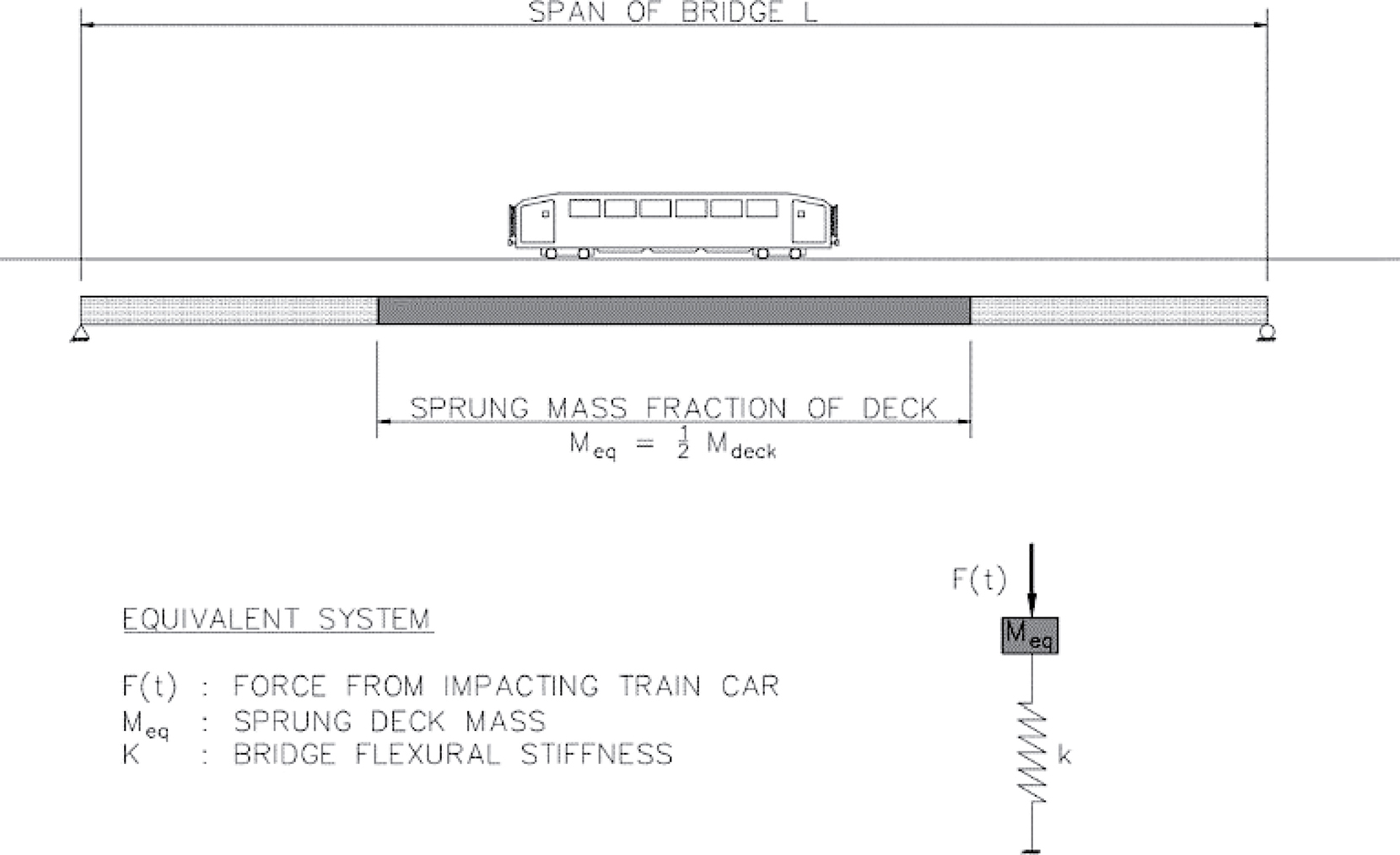
Long Description.
The diagram presents a simplified single degree of freedom bridge deck system. The top section shows a bridge span labeled as span of bridge L with a train car placed at the center. Below the bridge is a shaded region labeled sprung mass fraction of deck, marked as M subscript e q equals one half M subscript deck. The bottom right section displays an equivalent spring system with an arrow labeled F of t pointing down on a block labeled M subscript e q, which is connected to a spring labeled k. Text descriptions define F of t as force from impacting train car, M subscript e q as sprung deck mass, and k as bridge flexural stiffness.
Figure 14 illustrates the transition between the derailment simulations described in Chapter 3 and the impact analysis that uses the low-floor LRV baseline single rail break derailment as an example. The schematic demonstrates how the entire train mesh is transferred from the middle of the derailment simulation, and the post-impact derailment analysis is resumed on the flexible bridge deck to measure amplification due to the impact.
For the multi-car LRV trains, the horizontal, lateral, and angular velocities were applied to each car separately since the individual cars are allowed to pivot at the coupling joints and rotate independently. For the commuter rail vehicles consisting only of a single car, only one set of velocity parameters is applied to the entire train. An example of the transfer of velocity parameters between the two analysis simulations for the low-floor LRV single rail break scenario is shown in Figure 15. The velocities at the time step immediately before the initial impact are transferred to the start of the impact analysis simulation as initial conditions. After impact, kinematic deviations are noted because the vehicle interaction with the deck is allowed to displace vertically. However, the same motion trends and magnitudes are similar.
4.1.3 Deck Material
A range of analysis cases was performed on a rigid deck surface attached to the SDOF spring, which represents a conservative assumption that all the impact force is transferred into the structure of the bridge without any means of energy dissipation. To assess the validity of this assumption, the rigid deck was replaced with nonlinear concrete for the low-floor LRV single rail break derailment case to examine whether the energy absorption through plastic damage is significant. The nonlinear concrete was modeled with solid elements using the Karagozian & Case (K&C) concrete material model (i.e., LS-DYNA Material 72R3), with sufficient deck thickness to capture local deformations due to the impact. The K&C concrete material model, which captures damage and strain-rate effects, is commonly used in LS-DYNA for blast and impact analysis. An unconfined compressive strength of 4,000 psi was assumed.
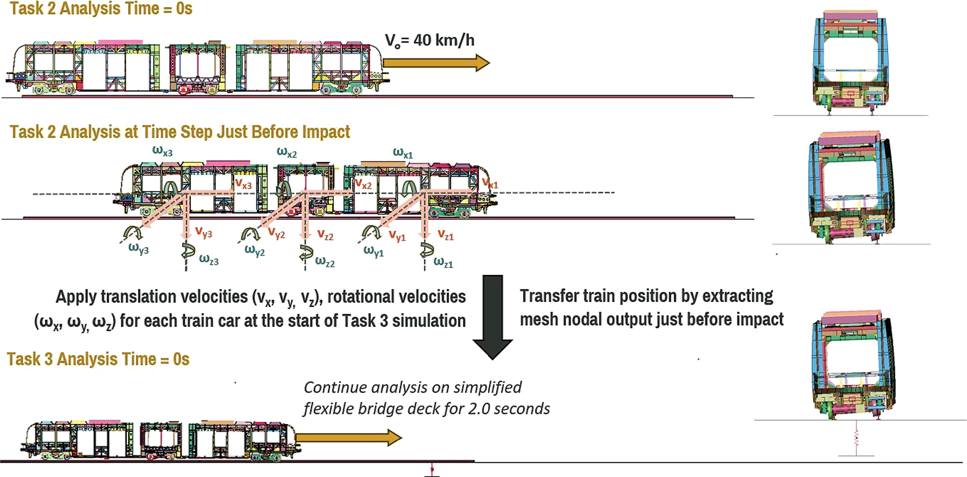
Long Description.
The diagram displays three stages of train impact simulation. The top section shows Task 2 analysis at time zero seconds, with a train moving at 40 kilometers per hour. The middle section shows Task 2 analysis at the time step just before impact, where each train car is labeled with translational velocities v subscript x, v subscript y, v subscript z and rotational velocities omega subscript x, omega subscript y, omega subscript z. Arrows show directions of motion for each train car. A thick arrow on the right indicates the transfer of train position by extracting mesh nodal output just before impact. The bottom section shows Task 3 analysis at time zero seconds, with the train continuing on a simplified flexible bridge deck. The analysis continues for 2.0 seconds. Front views of the train cars are shown on the right side of all three stages.
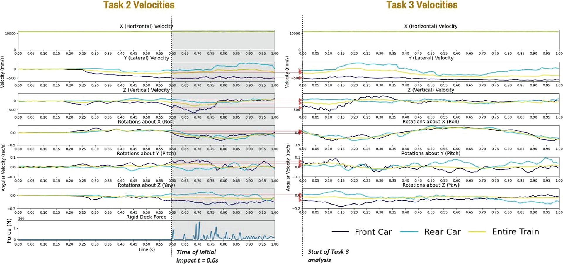
Long Description.
Two sets of seven vertically aligned plots labeled Task 2 Velocities and Task 3 Velocities. The horizontal axis in all plots is time in seconds, ranging from 0.00 to 1.00. Each plot shows three lines representing front car, rear car, and entire train. The top plot in each set is labeled X horizontal velocity with values ranging from 0 to 10,000 millimeters per second. Vertical dashed lines mark 0.60 seconds as the impact time in Task 2 and 0.00 seconds as the start of Task 3 analysis. All three lines remain nearly constant during Task 3 and show a gradual drop with disturbance near 0.60 seconds during Task 2. The second plot is labeled Y lateral velocity with a vertical axis from negative 500 to 0 millimeters per second. Task 2 shows a small initial drop, then variation post impact, while Task 3 shows more stable lateral movement. The third plot is labeled Z vertical velocity with a vertical axis from negative 500 to 0 millimeters per second. Task 2 exhibits sharp variation after 0.60 seconds, while Task 3 values remain relatively flat. The next three plots display angular velocities in radians per second about axes X roll, Y pitch, and Z yaw. Task 2 shows higher variation and larger fluctuations post impact, especially in the rear car and entire train. In contrast, Task 3 shows reduced angular response. The final plot under Task 2 is labeled Rigid Deck Force, with vertical values ranging from 0 to 1 newtons. Force spikes occur shortly after 0.60 seconds, corresponding to the marked time of initial impact. No force plot appears under Task 3. Overall, Task 2 reveals a significant dynamic response to impact, while Task 3 shows dampened behavior across all motion variables.

Long Description.
The diagram depicts a train model positioned on a rigid deck, transitioning onto a flexible section labeled, bridge spring. An arrow at the front of the train points toward the bridge spring section marked with non linear concrete elements. The bridge spring section is colored differently from the rigid deck and appears to include layered structural components. Labels identify the rigid deck, bridge spring, and non linear concrete elements. A 3D axis marker at the bottom left corner shows orientation along x, y, and z directions.
Figure 16 shows the model with a patch of nonlinear concrete elements in lieu of a rigid surface at the impact zone. The boundary edges of the solid concrete elements are kinematically constrained to move together with the surrounding rigid deck elements. The deck area with non-linear concrete is sufficiently large such that the boundaries are far enough away from the impact locations where local deformation is expected to occur. This simplified modeling approach only considers local deformation of the concrete caused by the derailment impact and assumes no additional deformation from global response. The results showed that the response of the bridge exhibited near identical behavior with nonlinear concrete as with the fully rigid deck, indicating that global stiffness governs the problem and local concrete deformation can be neglected.
4.1.4 Postprocessing
Dynamic amplification factors (DAFs) were determined as a ratio of the peak dynamic force to the static load. The peak dynamic force is determined by extracting the maximum force in the SDOF spring supporting the bridge deck, thereby neglecting static load from self-weight, dead load, and train weight. This step isolates out the additional force due to derailment impact only. Peak forces were compared with the corresponding static wheel load of the derailing truck, and subsequent falling trucks are not considered.
The current AASHTO LRFD Guide prescribes a derailment load factor of 100%, which implies a peak dynamic force equal to the static load. It is not specified in the guidelines whether the 100% derailment load factor is applied only to a single wheelset or the entire car simultaneously. The derailment scenarios considered in this research all occur in a single train truck because it is highly unlikely for a derailment to result in multiple trucks impacting the bridge deck simultaneously. Such extreme derailment events are outside the scope of this research.
4.2 Results and Discussion
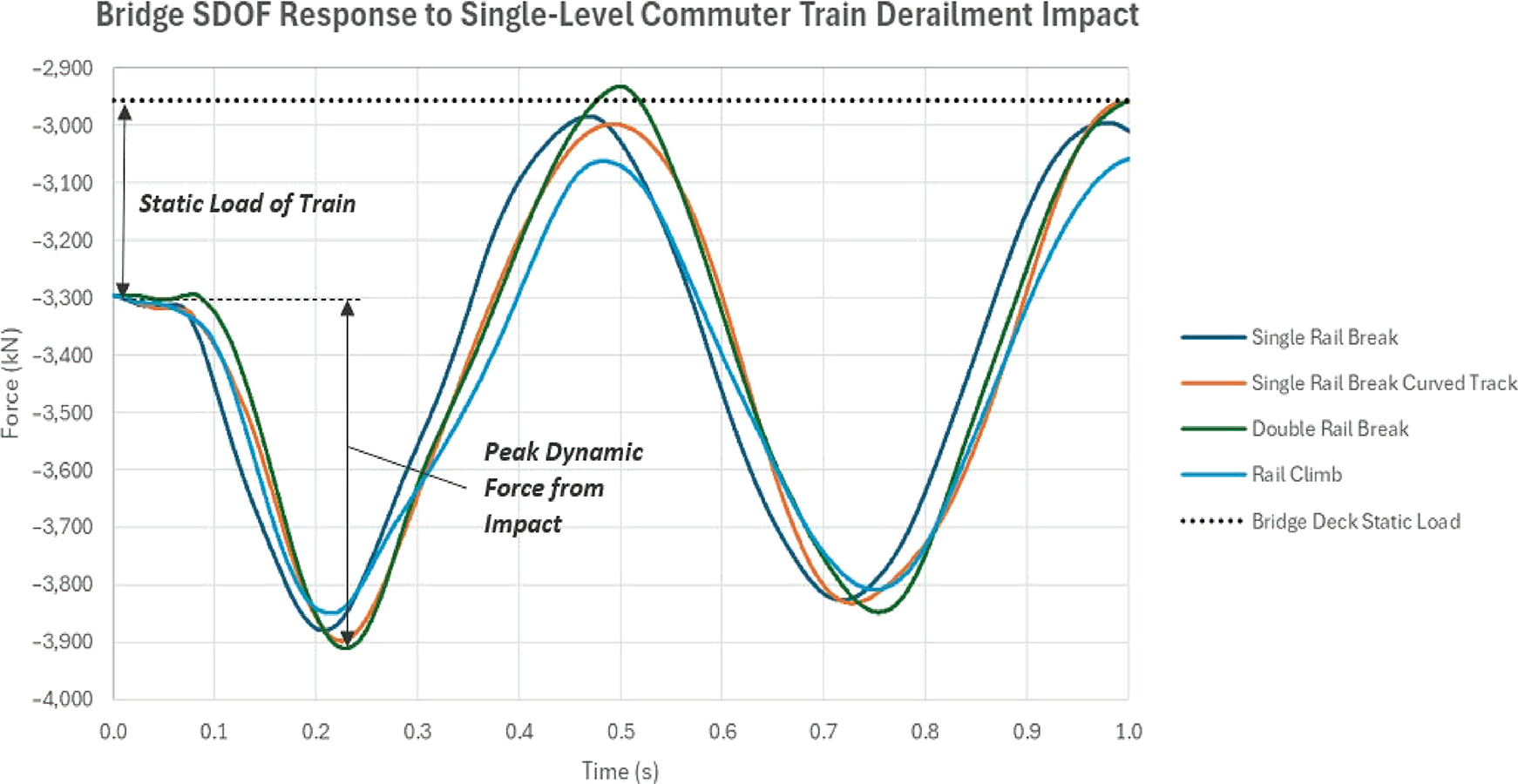
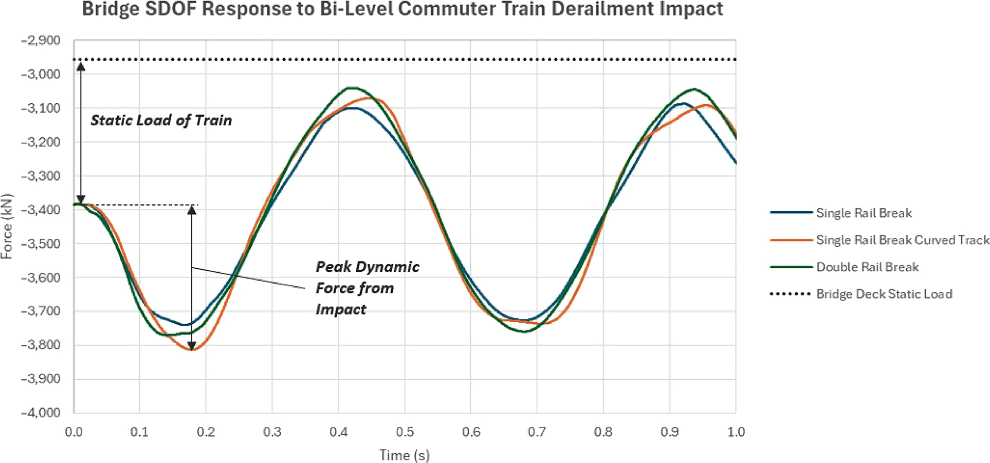
Figures 17 through 20 plot the force–time history in the bridge SDOF spring across all analyzed derailment scenarios for the low-floor LRV, high-floor LRV, single-level commuter, and bi-level commuter. The sinusoidal response is expected from an impulse load with a duration much shorter than the natural period of the bridge.
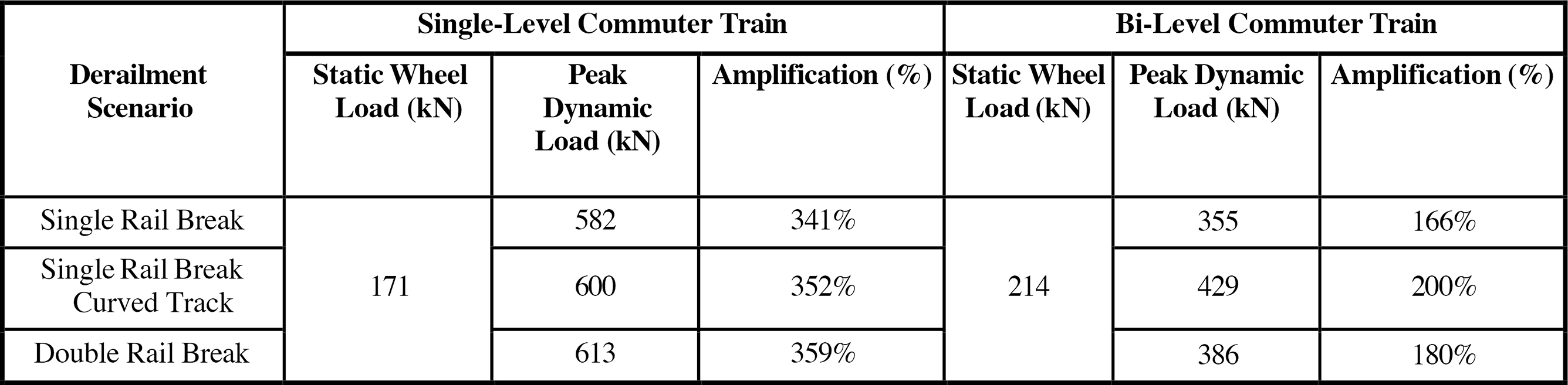
Tables 3 and 4 summarize the DAFs for all analyzed cases to date for the LRV vehicles and commuter cars. All preliminary amplification factors across all train models and derailment scenarios indicate a higher amplification ranging from 116% to 359%, further indicating a peak dynamic force of up to 3.5 times the static load.
Not much variance exists between the derailment scenarios within each train, and the governing derailment scenario varies for each train, which does not lead to any overarching conclusions about the importance of how the car derails. However, it is worth noting that for the high-floor LRV and the bi-level commuter car, which have higher centers of gravity, the effect of centrifugal force does increase the impact load more than the low-floor LRV and single-level commuter car.
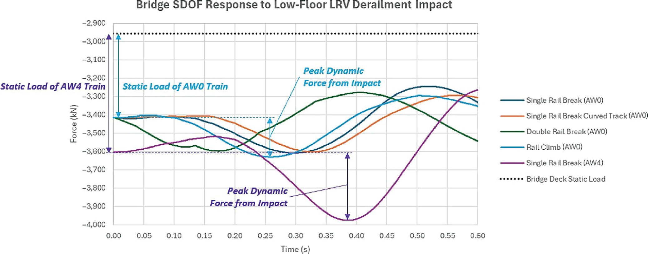
Long Description.
The graph plots force in kilonewtons on the vertical axis from negative 4,000 to negative 2,900 and time in seconds on the horizontal axis from 0.00 to 0.60. Six curves represent different derailment scenarios: single rail break AW0, single rail break curved track AW0, double rail break AW0, rail climb AW0, single rail break AW4, and bridge deck static load. The curve for single rail break AW0 has a dynamic peak force marked near 0.35 seconds. The curve labeled single rail break curved track AW0 also shows a peak dynamic force. The curve for single rail break AW4 shows the lowest point near 0.35 seconds. Dotted lines indicate static loads for AW0 and AW4 trains. Key force points, including static load and peak dynamic force, are labeled with arrows on the chart.

Long Description.
The graph plots force in kilonewtons on the vertical axis from negative 4,000 to negative 2,900 and time in seconds on the horizontal axis from 0.00 to 0.60. The force time responses shown are for high floor LRV derailment scenarios, including single rail break AW0, single rail break on curved track AW0, double rail break AW0, rail climb AW0, and single rail break AW4. The bridge deck static load is represented by a horizontal dashed line near negative 2,950 kilonewtons. For single rail break AW0, the force starts near negative 3,400 and oscillates with a peak near 0.30 seconds. For single rail break curved track AW0, the force dips to about negative 3,650 and peaks just after 0.30 seconds. For double rail break AW0, the curve shows a mild dip and peak between 0.20 and 0.40 seconds. The rail climb AW0 curve shows oscillation similar in shape to single rail break AW0, but with a slightly lower peak. The single rail break AW4 curve dips to a lowest force value near negative 3,900, between 0.25 and 0.30 seconds. Arrows and text mark static load of AW0 train and AW4 train at the start, and peak dynamic forces from impact for both AW0 and AW4 cases between 0.25 and 0.30 seconds.
Long Description.
The graph plots force in kilonewtons on the vertical axis from negative 4,000 to negative 2,900, and time in seconds on the horizontal axis from 0.0 to 1.0. It presents the bridge single degree of freedom response to single level commuter train derailment. The four curves represent single rail break, single rail break curved track, double rail break, and rail climb. All curves begin near negative 3,400 and dip below negative 3,900 between 0.2 and 0.3 seconds, marking the peak dynamic force from impact. They then rise toward a peak between 0.4 and 0.6 seconds, then decline again toward the end. A horizontal dashed line represents the bridge deck static load near negative 2,950 kilonewtons. An arrow identifies the static load of the train near the start, and another arrow marks the peak dynamic force from impact between 0.2 and 0.3 seconds. The curves maintain similar shape and timing across all derailment cases.
Long Description.
The graph plots force in kilonewtons on the vertical axis from negative 4,000 to negative 2,900, and time in seconds on the horizontal axis from 0.0 to 1.0. It represents a bridge single degree of freedom response to bi level commuter train derailment. Three curves are shown for single rail break, single rail break curved track, and double rail break scenarios. All three curves begin around negative 3,400 and dip to approximately negative 3,850 between 0.1 and 0.2 seconds, marking the peak dynamic force from impact. The curves then rise to near negative 3,100 around 0.45 seconds and follow a second wave of dip and rise. A horizontal dashed line near negative 2,950 marks the bridge deck static load. An arrow identifies the static load of the train near the beginning of the graph, and another arrow highlights the peak dynamic force from impact. The force patterns are similar across all three scenarios.

Long Description.
The table presents data for low floor LRV and high floor LRV under two passenger load cases labeled AW0 and AW4. Column headers include Passenger Load Case, Derailment Scenario, and under each vehicle type there are three subscript-columns: Static Wheel Load in kilonewtons, Peak Dynamic Load in kilonewtons, and Amplification in percent. For AW0 and low floor LRV, the static wheel load is 154 kilonewtons. Under single rail break, the peak dynamic load is 194 and amplification is 126 percent. Under single rail break curved track, peak dynamic load is 188 and amplification is 122 percent. Under double rail break, peak dynamic load is 183 and amplification is 119 percent. Under rail climb, peak dynamic load is 215 and amplification is 140 percent. For AW4 and low floor LRV, static wheel load is 222 kilonewtons, peak dynamic load is 372 and amplification is 168 percent under single rail break. For AW0 and high floor LRV, static wheel load is 159 kilonewtons. Under single rail break, peak dynamic load is 206 and amplification is 129 percent. Under single rail break curved track, peak dynamic load is 271 and amplification is 170 percent. Under double rail break, peak dynamic load is 185 and amplification is 116 percent. Under rail climb, peak dynamic load is 227 and amplification is 143 percent. For AW4 and high floor LRV, static wheel load is 218 kilonewtons, peak dynamic load is 295 and amplification is 135 percent under single rail break.
Long Description.
The table presents derailment data for single level commuter train and bi level commuter train across three scenarios: single rail break, single rail break curved track, and double rail break. Column headers include Derailment Scenario, and under each train type there are three subscript-columns: Static Wheel Load in kilonewtons, Peak Dynamic Load in kilonewtons, and Amplification in percent. For single level commuter train, the static wheel load is 171 kilonewtons. Under single rail break, the peak dynamic load is 582 and amplification is 341 percent. Under single rail break curved track, peak dynamic load is 600 and amplification is 352 percent. Under double rail break, peak dynamic load is 613 and amplification is 359 percent. For bi level commuter train, the static wheel load is 214 kilonewtons. Under single rail break, the peak dynamic load is 355 and amplification is 166 percent. Under single rail break curved track, peak dynamic load is 429 and amplification is 200 percent. Under double rail break, peak dynamic load is 386 and amplification is 180 percent.
Regarding the effect of passenger load, the low-floor LRV with an AW4 load increases the amplification from 126% to 168% for the baseline single rail break scenario, while the high-floor LRV sees a smaller change from 129% to 135%. Based on previous research, the passenger load was not expected to significantly alter the dynamic amplification since the mass is evenly distributed across the train cars.
4.2.1 Effect of Bridge Frequency
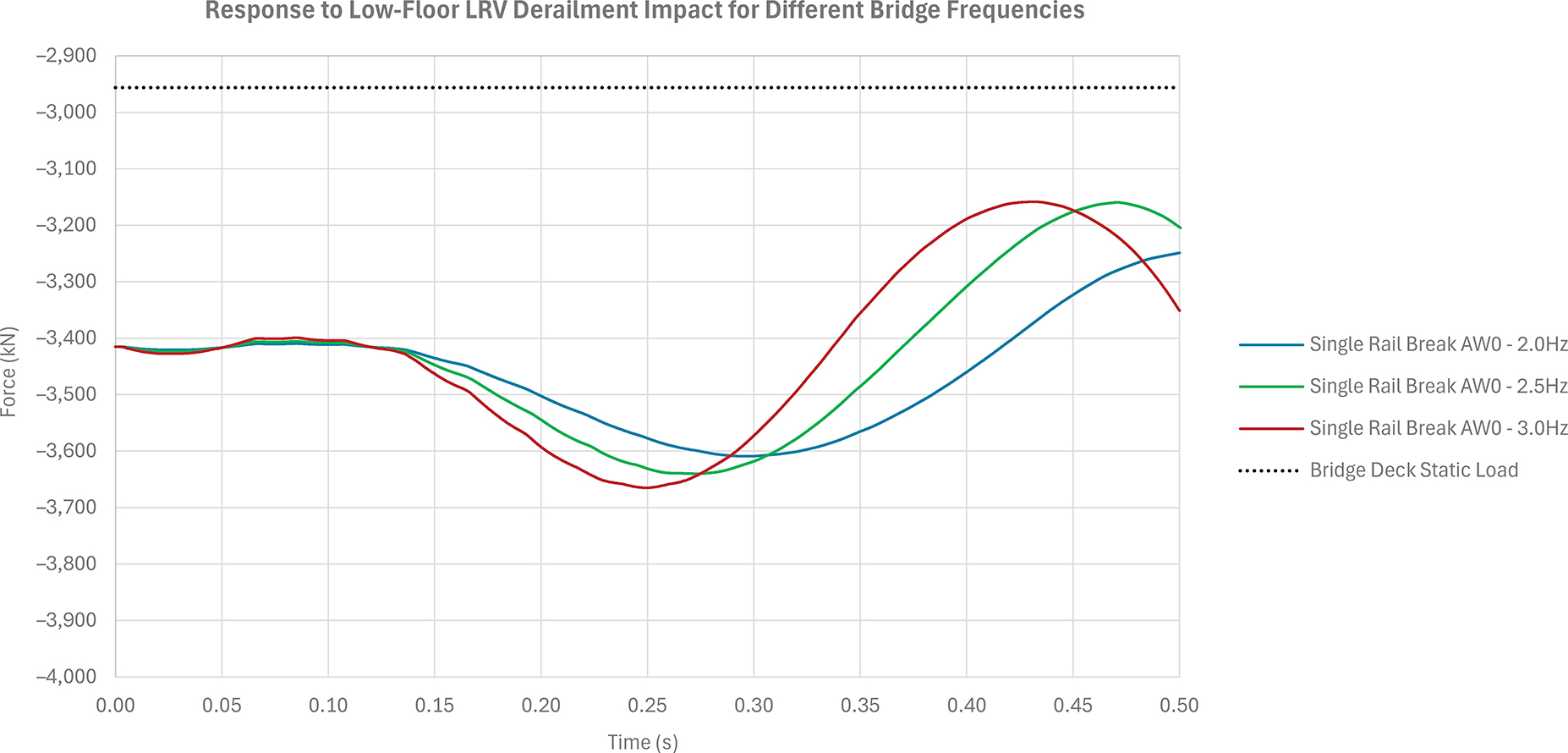
The natural frequency of the example bridge structure, which accounts for structural weight and superimposed dead loads, was 2.0 Hz, which corresponds to a position near the lower bound of typical transit bridges. Two additional bridge models were considered to determine the sensitivity to the bridge frequency. The stiffness of the two models was recorded as 82.5 kN/mm (471 kip/in.) and 120.0 kN/mm (685 kip/in.), which corresponds to the natural frequencies of 2.5 Hz and 3.0 Hz, respectively, with all other properties remaining unchanged. This sensitivity study was performed with the low-floor LRV train for the baseline single rail break derailment scenario with an AW0 load; the results are shown in Figure 21. The dynamic amplification increases from 126% for the original 2.0 Hz structure to 146% for the 2.5 Hz structure and 163% for the 3.0 Hz structure. These findings are consistent with previous studies focused on the simplified derailment impact.
Long Description.
The graph shows force in kilonewtons on the vertical axis from negative 4,000 to negative 2,900 and time in seconds on the horizontal axis from 0.00 to 0.50. Three curves represent the response of low floor LRV under single rail break AW0 condition for different bridge frequencies: 2.0 hertz, 2.5 hertz, and 3.0 hertz. A horizontal dashed line at approximately negative 2,950 marks the bridge deck static load. All curves begin around negative 3,400 and show a dip in force, in the range from 0.25 and 0.30 seconds, followed by a rise toward 0.45 seconds. The 2.0 hertz curve shows the least oscillation, while the 3.0 hertz curve shows the greatest change with the deepest dip and highest peak. The 2.5 hertz curve lies between the other two. All curves illustrate the dynamic response variation due to bridge frequency.


