Data Fusion of Probe and Point Sensor Data: A Guide (2024)
Chapter: 5 Data Fusion Framework
CHAPTER 5
Data Fusion Framework
The goal of sensor and probe data fusion is not fusion in and of itself. Instead, fusion is performed to improve quality or value of individual datasets, or to extract new insights otherwise not evident from individual datasets—especially by the creation of new datasets or merging of disparate data. The fusion methods described herein are applicable to sensor and probe data and are likely more applicable to probe and point-sensor data and transportation use cases. This paper also focuses on methods that are reasonably implementable and provide the likely best value for agencies.
The data fusion framework is specifically tailored to the fusion of point sensor and probe data. There are four high-level steps in the framework, shown in Figure 9:
- Pre-Processing
- Spatial and Temporal Alignment
- Region- and Use Case-Specific Algorithm
- Quality Control and Feedback
The framework is a set of detailed, step-by-step instructions on how to prepare, clean, fuse, and perform quality control on the data. Within each step, highlighted by red boxes in Figure 10, this framework procedure provides short examples of how to apply each step of the framework. An executive summary also describes, at a high level, the purpose and importance of each step—including

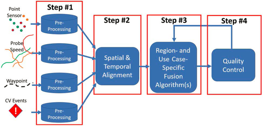
what can happen if the step is ignored or improperly implemented. For each of the high-level steps in Figure 9, there are specific and detailed explanations of items such as:
- How to format data
- Specific inputs required
- How to manipulate the data for different algorithms
- How to check for outliers (without throwing out good data)
- Cleaning
- Additional steps for use case-specific fusion algorithms.
5.1 Step #1: Prepare Data (Pre-Processing)
5.1.1 Executive Summary
The first step in data fusion is the prep work related to making sure the data fused are in the correct format, are of an acceptable quality, etc. This step is analogous to the prep work when getting ready to paint a room in a house. Prep work for painting might include tasks like:
- Selecting the right type of paint for the wall surface—including the proper finish (eggshell, glossy, matte, etc.)
- Selecting the right type of brushes and rollers for the desired finished look and surface conditions
- Sanding and priming surfaces
- Moving furniture away from walls
- Covering the floors with drop cloths
- Masking areas that are not to be painted
When painting a room, this prep work takes a lot of time and can be 75% of the labor. But if it is not done well (or at all), then the results are usually not great, expensive items in the room can get ruined, and the job may take longer than it should. The room may even need to be repainted later because the wrong color or wrong types of brushes and rollers were selected.
Just as prep for room painting is important for successful results, pre-processing data is a critical step in the data fusion process. If pre-processing is not done or is only partially completed,
poor quality data and compromised data will be used in the following fusion steps, amplifying all those poor qualities and errors and producing inaccurate or nonsensical results.
5.1.2 For the TSMO Professional
Data Fusion pre-processing includes the following tasks:
- Assessing the quality of the data
- Tagging and/or cleaning the data
- Normalizing and/or formatting the data for easier use
Each of the four types of datasets shown to the left of the “Pre-Processing” step in Figure 11 have widely varying steps required to pre-process them. For example, point sensors are usually installed, calibrated, and managed by each individual DOT. Because of this, the DOT may have more insights into quality issues with the sensors. Sensors may have also been deployed years apart, meaning there will be different sensor models, potentially different technologies used, different polling intervals, etc. The DOT will have less visibility into data procured from third party probe providers that can sometimes seem opaque. This includes data from probe speed vendors, waypoint data, and CV event data.
Spending enough time on Step #1 of this data fusion process will help to ensure that the remaining steps are easier, that the final outputs are of higher quality, and that the effects of the “garbage in, garbage out” problem of data fusion are reduced.
Pre-processing data does not always mean removal of lower quality or data otherwise deemed “bad.” Certain use cases may make use of lower-quality data as long as they do not dominate the overall dataset, they are properly documented and communicated, and the fusion outcomes have low sensitivity or are focused on approximations and overall trends rather than precise values. The fusion algorithm may have quality thresholds that ensure that only an acceptable quantity or quality of input data is used. “Bad” input data can be tagged appropriately, and results tagged to indicate lower quality data were utilized. Alternatively, “bad” data can be excluded entirely or replaced by imputed data.

5.1.3 Specific Implementation Guidelines
Pre-processing steps are specific to the type of data prepared for fusion. Below are specific implementation guidelines for the four main sources of data covered in this document.
5.1.3.1 Point-Sensor Data
Point-sensor data are generally produced by physical sensors installed in the pavement or near or over the roadway being monitored. In-pavement sensors collect data by detecting vehicles passing over them, while side-fired and overhead sensors use radar, acoustic, or other methods to detect vehicles and capture their speed and other vehicle parameters. The usefulness for the resulting data is directly related to sensor accuracy, calibration, communication reliability, and environmental conditions. Therefore, the first step in preparing point-sensor data may be to evaluate the sensor device inventory and decide which sensors may need to be excluded or handled separately due to known issues (e.g., malfunctions, miscalibrations, inactivity due to construction).
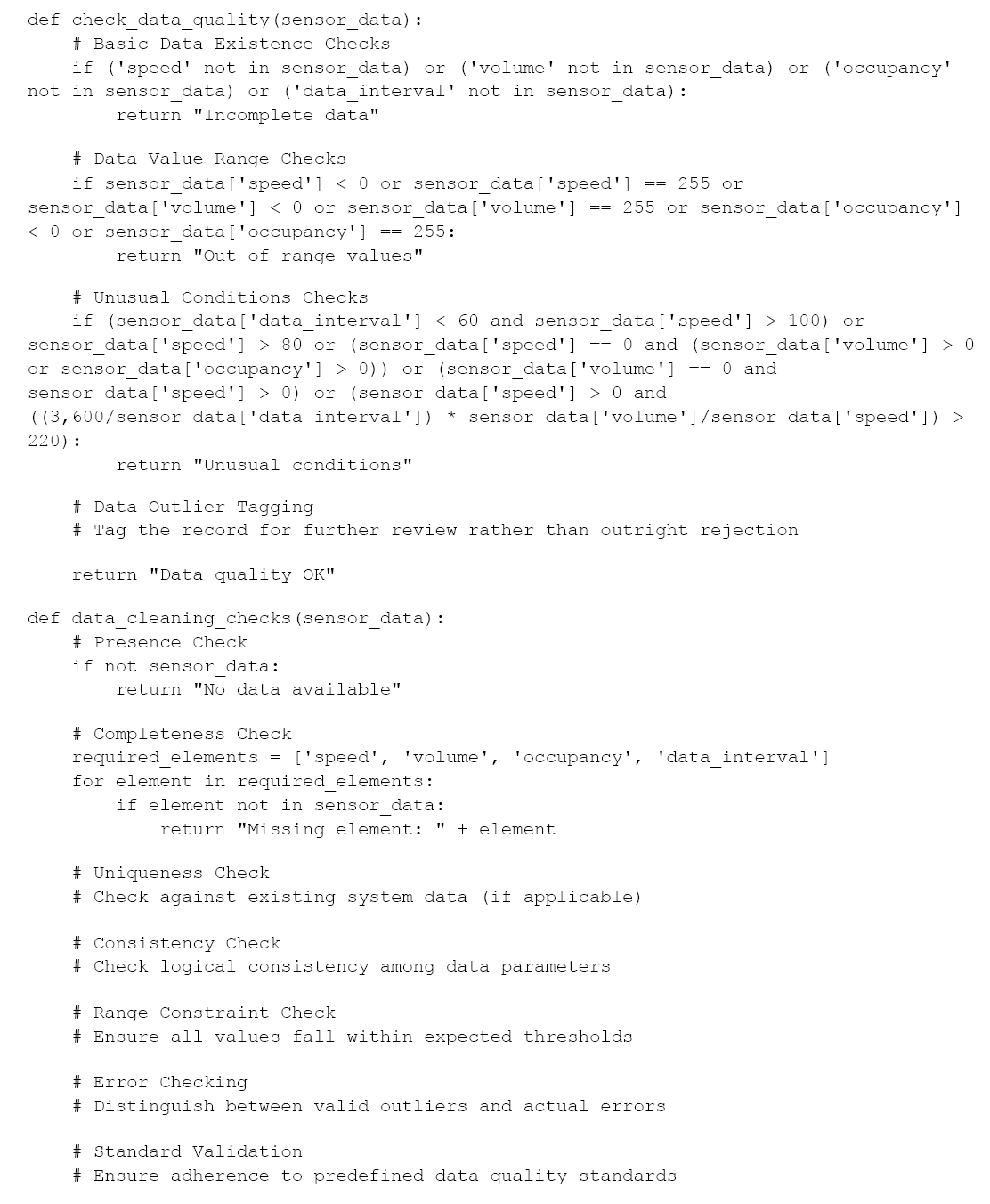
Incoming real-time data must be evaluated for validity and applicability for fusion. The first set of validity checks includes logical checks for values that make sense. Cambridge Systematics and Texas A&M Transportation Institute (TTI) published recommendations for logical quality control procedures for per-lane sensor data to capture potential invalid records in real time (Turner 2007). These checks include the following:
- Speed does not exist
- Volume does not exist
- Occupancy does not exist
- Data Interval does not exist
- Speed is −1 OR speed is 255 OR volume is −1 OR volume is 255 OR occupancy is −1 OR occupancy is 255 (255 is the largest integer value that can be stored in one byte of data)
- (3,600/Data Interval * volume) is greater than 3,000
- Data Interval is less than 60 seconds AND speed is greater than 100 mph
- Speed is greater than 80 mph
- Speed is 0 mph AND volume and occupancy are greater than 0
- Volume is zero and speed is non-zero
- Speed volume and occupancy are all 0
- Speed is greater than zero and [(3,600/Data Interval * volume)/speed] is greater than 220
These quality controls can be tailored and/or supplemented based on individual sensor systems and roadway infrastructure. For example, sensors that aggregate data across several lanes of traffic (frequently defined as a “zone”) may require per lane checks to be aggregated accordingly before executing the volume data logical checks. Similarly, roadways with speed limits more than 80 mph would require adjustment to “Speed is greater than 80” check to use a more reasonable value.
Captured values that fall outside of these logical tests must be handled based on the data fusion strategy an agency is implementing. For fusion algorithms that use only valid and verified data, the values that fail logical tests would be excluded. The downside of this approach is that there could be data gaps that make the fusion process more difficult or impossible, resulting in overall fusion data gaps. On the other hand, invalid data could be tagged as invalid or “questionable” and used in the fusion algorithm with results equally tagged to indicate that the values may not be accurate. The benefit of doing this is avoiding data gaps, but the resulting fused data results must consider the quality tag depending on use case (e.g., real-time safety applications may exclude any tagged data, while less precise aggregated data use cases may allow for a certain amount of tagged data to be included). Finally, invalid values could be replaced by imputed values (and tagged accordingly) to avoid data gaps as well as clearly invalid results. Various imputing algorithms can be utilized to generate imputed values, such as probabilistic model-based methods,
e.g., probability principal component analysis (PPCA); regression model-based methods, e.g., linear regression, support vector machine (SVM), and neural networks (NN); and matrix completion-based methods, e.g., low-rank matrix completion (LRMC) (Chen, et al. 2018).
Beyond the individual values’ logical checks, there are several other point-sensor data checks that need to be executed before proceeding with using that data in various fusion algorithms. These checks include the following:
- Presence: Are entire expected records missing? For example, if the sensor is supposed to report data once per minute, and if a record is not captured for that time interval, the gap needs to be addressed in one of two ways: (1) carry the gap through the fusion with the resulting fused data having the same gap; and (2) impute the missing values and tag them accordingly.
- Completeness: Are all required and/or expected elements present? A sensor may report some values while missing others. For example, a sensor may capture the speed value, without volume or occupancy values. In this case, the logical checks may determine whether data are invalid, or previously known information (such as miscalibration or sensor system capability) may determine that the speed value can be utilized in a data fusion algorithm that relies on speed data only.
- Uniqueness: Are the data already present in the system? There are three ways to evaluate uniqueness. First, if the incoming data record has all data elements equivalent to an existing record (including unique ID and timestamp), then that record must be considered duplicate and discarded or imputed. Second, if the incoming data record has a duplicate unique ID or timestamp, but different data values, then that record must be further evaluated to determine whether the device is defective or if the network issue resulted in erroneous duplication of ID and timestamp data. The third case involves unique ID and timestamp, but measurements that match the previous measurements. This case may be difficult to evaluate in real time as repeated values may be perfectly normal and acceptable. For example, if a sensor is reporting speed of 60 mph for several consecutive intervals, that may reflect the true conditions on the roadway. However, if the repeating pattern appears over a long time period or is verified not to make sense based on complementary data sources (e.g., closed-circuit television [CCTV], incident detection system) then those records may need to be excluded or imputed accordingly.
- Consistency: Do the data make logical sense? Most of these checks are covered logical quality checks described in the previous section, but can be customized based on specific devices, vendors, and environment in which the sensors operate.
- Range Constraint: Do all values fall within the expected threshold? Similarly, these checks are covered by logical quality checks described in the previous section.
- Error Checking: Is an outlier a valid reading or an error? Error checking is covered by the logical quality checks described in the previous section.
- Standard Validation: Do the data conform to a given standard? This validation step is often not necessary when data are pulled directly from the field device, but it is commonly used when sensor data are reported by a third party managing or maintaining the field device. In those cases, an application programming interface (API), webservice, file transfer protocol (FTP), or a similar method is used to deliver data conforming to a specific data standard or format. This step validates that incoming data conform to the specified data standard or format and, if validation fails, the data snapshot may not be valid.
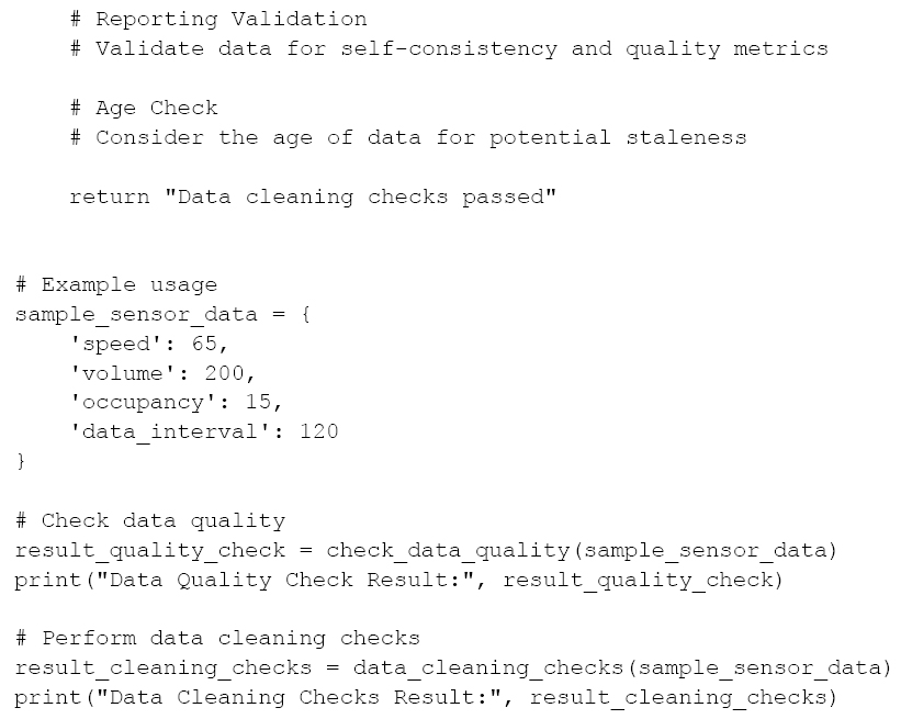
- Reporting Validation: Are data self-validating and providing a quality metric? Field devices often contain a quality flag that indicates potential issues such as loss of communication, incorrect operational mode, configuration error, etc. When a device self-reports one or more of these flags as true, the incoming data must be considered accordingly.
- Age: Are data considered stale after a certain amount of time? Most field devices report data in a preset time interval. If additional latency is introduced due to network issues, device
malfunction, or issues with the receiving system, the incoming data may be stale. In other words, it may be reporting data from past time intervals, which could range from a few minutes ago to hours ago. Based on the real-time needs of the fusion use cases, stale data may not be acceptable input to the fusion algorithm.
5.1.3.2 Probe Speed Data
Unlike point-sensor data, probe-based speed data from the private sector is more difficult to evaluate in real time because the methods by which it is produced are generally hidden from end users. Most data quality evaluations of probe-based speed data are conducted after the fact using Bluetooth or Wi-Fi reidentification data. TETC developed many of these validation methods (Young 2015) (I-95 Corridor Coalition 2017) (TETC 2020). These validation efforts are performed at discrete locations and are usually done for about a week at a time.
For real-time data quality control, most probe data providers give users a pre-computed quality indicator or confidence score. These scores can be indicative of the following:
- High Confidence: The provider has one or more probes traveling on the roadway during the reporting period which are used to produce speed measurements.
- Medium Confidence: Probes are not present on the specific road segment, but may be just upstream or downstream, and the amount of time passed since seeing a probe is relatively short.
- Low Confidence: It has been many minutes since any probes have driven this segment, and there are no probes upstream or downstream. The speed reading is likely a reversion to historic speeds or even the reference speed for this segment.
When evaluating the quality of probe-based speed data in real time, the user has to trust that the provider’s self-reported scores during the pre-processing step in the fusion framework methodology. These self-reported confidence scores can be used to flag data of low confidence that may be questionable for use in a fusion algorithm. Note that medium-confidence data are potentially adequate for some applications and that even low-confidence data may be useful during certain times of the day. For example, one may expect high-confidence data during peak periods on high-volume roads; however, during early morning hours on low-volume roads, medium- and low-confidence data may be good enough for certain applications.
In addition to the self-reported confidence scores, agencies can look for a few other indicators of potential problems with probe data. These can include:
- Data Age: Probe data providers usually provide an updated speed reading every 1 or 2 minutes. These data should be provided with a timestamp. Agencies will need to check these timestamps to ensure that they are correct and timely. Data should not be old or stale—which could be an indicator of a malfunctioning data feed.
- Data Presence: Most vendors will provide speed values for all segments at the same time. If a large number of segments are being dropped from the data feed, this is indicative of a data issue.
- Data Gaps: If the vendor is expected to provide data every minute of every day, and there are gaps of 5 minutes, 10 minutes, etc., between new measurements, then the data should be flagged. Some use cases may not require data every minute, but some use cases may break down and cease to function if too many gaps exist.
- Range Consistency: Most probe data providers cap speed readings at some value—for example, 80 mph. Therefore, if unreasonably high speeds (or unreasonably low speeds including negative speeds) are being reported, there is likely an issue with the data feed.
- Variability: While uncommon, a fluctuating set of speed readings could be indicative of a problem with data. For example, speeds that alternate every couple of minutes between high
and low values or in other patterns that are unlikely to occur in reality may be incorrect. Speeds fluctuating between 60 mph and 10 mph that switch every 1–2 minutes are unlikely.
5.1.3.3 Waypoint Data
Waypoint data, like probe-based speed data, come largely from the private sector and can be difficult to evaluate for quality without significant effort. Waypoint data should not be confused with O-D data and the efforts being developed to validate them (TETC 2023). Most waypoint data obtained directly from CVs are considered accurate and trustworthy so long as the original pings/waypoints are relatively frequent as to not require the provider to have to estimate routing and/or insert estimated waypoints. These CV waypoints represent actual experienced trips from real-world vehicles.
However, quality cannot be guaranteed for waypoint data derived from LBS providers. Leading up to and through the early days of the COVID-19 pandemic, LBS data were growing in quantity and popularity. Data from companies were prevalent, cheap, and trustworthy. However, with negative press and the changing political climate toward the tracking of individuals, many of these providers lost access to their source data. These data providers get paid per device tracked. In an effort to keep revenues up, less scrupulous providers began faking or synthesizing data. Weeding out these fictitious data is time consuming and nearly impossible. Checking data quality entails looking for roads that are closed or traveling well below the reference speed, and searching for waypoints and trips that “break through” closed roads en masse or travel at otherwise improbable speeds during rush hour or times when incidents create severe congestion. No known algorithm exists at the time of the writing of this report that can check the quality of waypoint data derived from LBS data without significant manual intervention. For this reason, it is recommended to avoid the use of these types of data—opting instead for waypoint data derived from CVs only.
5.1.3.4 CV Events
Checking for quality issues with CV event data is also difficult. Airbag deployments have to be assumed to be accurate until disproved with field responders. Weather data from CVs can be checked against road weather information system (RWIS) stations or National Weather Service (NWS) radar, but can be tricky since radar searches for weather disturbances in the atmosphere while CVs detect ground weather events, e.g., wet road surfaces and fog. Similarly, RWIS stations are spaced few and far between, and may miss localized weather conditions detected by vehicles traveling directly on roadways far away from RWIS sites.
Heavy braking and rapid acceleration event data are commonly available CV event data types. Some vendors and OEMs can provide these data in real time where others are provided only at key-off. Regardless of when the data are received by an agency, there needs to be careful consideration of how the data provider classifies heavy braking and/or rapid acceleration vs. what the agency may define as heavy braking and acceleration. Acceleration and deceleration rates that trigger events by the provider may not be appropriate for all classes of roadways. For example, heavy braking on an interstate vs. heavy braking on a roadway where signals and stop signs and sharp turns may warrant different definitions as they have different impacts on safety. Depending on the application, the research team may need to consider the definition of event (e.g., heavy braking) and think about whether the vendor’s and the DOT’s definitions agree.
CV events can also include weather-related occurrences such as fog and rain detection. Airbag deployments can be provided by other vendors, and some can even provide lane departure warnings. This is a rapidly evolving and changing data source—and the evolution is not always in the positive direction. Checking the quality of these data can be difficult. A committee within TETC is forming as of the writing of this report to try to determine what can be done, but the work is only just beginning.
5.1.4 Examples of Implementation
Examples of Python code for checking the quality of speed sensor data before sending it on to Step #2 in the framework follow. Depending on one’s preferred programming language and context of use, this code can be adapted and further developed to suit the requirements of a specific system or application.
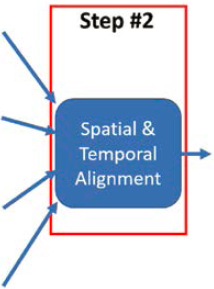
5.2 Step #2: Spatial and Temporal Alignment
5.2.1 Executive Summary
In old foreign-language films that have been dubbed, or a video call with poor Internet connection, the importance of spatial and temporal alignment is demonstrated. As moving pictures tell a story, whether a fictional one or one reporting the most recent quarter’s earnings, if the associated audio is offset by even a fraction of a second it becomes almost impossible to follow and comprehend the story. The mind struggles to reconcile the difference between what is seen and what is heard due to misalignment of video and audio.
Spatially and temporally aligning detector and probe data is equally important in telling a data story. Like misaligned video and audio, detector data at one spatial or temporal scale cannot be used with probe data at another spatial or temporal scale without some sort of alignment process. Using misaligned datasets will result in inaccurate, misleading, or plain wrong outcomes. Aligning diverse datasets enables a comprehensive view and a deeper understanding of the underlying patterns, trends, and relationships within the data.
Step #2 (Figure 12) describes approaches to aligning the sensor and probe data both spatially and temporally. These are referred to as spatial data fusion and temporal data fusion. While they both happen in Step #2, they are separate processes, each as important as the other.
5.2.2 For the TSMO Professional
Detector data and probe data are collected in the field using different protocols and methodologies resulting in various temporal and spatial scales for various datasets. In addition, as data are ingested into various systems, it may be further aggregated or processed, changing its
temporal and/or spatial properties. To effectively utilize these disparate scale datasets, data must be temporally and spatially fused.
Temporal fusion targets datasets that may be collected, made available, or aggregated to different time periods. For example, detector speed data may be collected in 1-minute intervals in the field, but then aggregated to 5-minute intervals for use by operators and aggregated to hourly time intervals for use in planning applications. On the other hand, probe speed data may be only available in 5-minute intervals due to the way a third-party provider packages data in their product or due to contractual agreement that dictates the granularity of data. In order to utilize these two datasets, it is important to temporally fuse them to a common time interval or to associate them to a common time interval based on other properties. This becomes even more important when temporally fusing detector data collected on a set time interval (e.g., 1 minute) with CV event data, which may be asynchronous (i.e., generated when an event occurs rather than on a set schedule) and often unavailable in real time.
Equally important, spatial fusion targets datasets that may be collected, made available, or aggregated into different spatial scales. For example, a point detector may be collecting per-lane data at a specific point location along the roadway. A downstream system, like an ATMS platform, may be aggregating that per-lane data into “zones” that cover multiple lanes at a specific location. On the other hand, probe speed data are generally collected along a segment of roadway defined by a start and end point. Segments often vary in length based on roadway location, class, and by probe data vendor. To use detector data with probe data, it is important to determine how those detector point locations relate to variable segments, and how do data collected at a single point relate to the “averaged” data along a segment.
The risk of not aligning data across temporal and/or spatial scales, or doing so incorrectly, can result in misleading or incorrect fusion results and potentially incorrect decisions based on that fused data.
Table 5 shows the different time scales and coverage areas for point sensor, probe data, and CV event data.
5.2.3 Specific Implementation Guidelines
5.2.3.1 Spatial Data Fusion
Spatial fusion involves evaluation of multiple elements from different records and data sources, and making meaningful spatial connections between those records. Those connections can then help to derive further information or insights, such as correlation and causation, impact, and potential outcomes. Spatial fusion uses context to set thresholds for relating spatial components of disparate data records. For example, spatial fusion may be performed to relate data from a specific static roadway sensor to a roadway segment along which a probe travel time is reported or a probe vehicle event is detected. The fusion method may include defining appropriate geospatial buffers for a given sensor and segment that ensure that appropriate sensor/segment pairs are linked while accounting for density of sensors and segments. In other words, in an urban area, sensors may be densely spaced and segment lengths may be short, which may result in aggressive spatial buffers that ensure no extraneous segments or sensors are included when data are fused. Conversely, in a rural area, sensors may be sparsely located and segment lengths may be large, which allows for larger spatial buffers to account for location errors, but also introduces potential quality concerns resulting from extrapolation of information from low-resolution data.
Spatial alignment (conflation) of probe data and detector data is not a straightforward activity and often includes many outliers. In other words, an algorithm may be developed to address a large majority of conflation cases, but may miss certain special (but common) cases, such
Table 5. Spatial and Geographic differences in point sensor and probe-based data.
| Measurement Location | Measurement Timing | |
| Point-Sensor Data | At a single location on the roadway in the center of each lane or at a spot representing the sum and average of all lanes at a single location usually represented by latitude/longitude coordinates. | Highly variable depending on the agency and sensor. Could be every few seconds, every 20 seconds, every minute, every 5 minutes, etc. |
| Probe-Based Speed Data | A speed reading representing a segment of the roadway where segments can be hundreds of meters or several miles in length. | Most data providers produce a new measurement every minute, but depending on the product or contract agreement, measurements may be provided in less granular time periods (e.g., 5 minutes). |
| CV Event Data | Weather events can be at single locations or covering a polygon of any shape and size. Other events can be at discrete locations on the roadway represented by latitude/longitude coordinates. | Can be in near real-time as events are detected, or they can be provided in batches at key-off or at the end of a day. |
| Probe-based Waypoint data | Waypoints are usually single points represented by latitude/longitude coordinates, but can occasionally be segment-based. | The waypoints are usually collected at regular intervals that can range from several seconds apart to 30 seconds or minutes apart. Regardless of the collection frequency, providers may transmit the waypoints to a user in real-time or daily/monthly depending on the provider and contract terms. |
as roadways with multiple names and aliases, beltways/loops with various direction and name schemes, and so forth. This is largely caused by detector metadata quality issues and different probe data segmentation definitions and differences in map products and versions. Map products and versions are a significant factor as different vendors release updates on different schedules and the updates can vary from simple new segment additions to represent new pavement, to much more difficult to manage segment removals or resizing due to changes in data collection methods and pavement changes.
Generally, point sensor metadata includes the following elements relevant to the conflation process:
- Detector ID—unique ID for the detector controller.
- Zone/Lane ID—unique ID for individual lanes or aggregated zone in that location.
- Road—road name or other road designation.
- Direction—direction of travel being monitored.
- Location Description—brief location description, often based on intersecting features such as (I-495 @ MD-212)
- Zone/Lane Type—description of the lane/zone type, such as “general purpose” or “shoulder” or “on-ramp.”
- Detector Type—type of detector device, such as radar, microwave, acoustic, etc.
- Latitude
- Longitude
Less frequently, point sensor metadata may include additional spatial elements that could be useful in conflation such as:
- State
- County
- City
- ZIP Code
- Intersecting Feature—intersection, interchange, mile marker, etc.
Sensor metadata may include many other elements, but they may not be relevant to the spatial conflation process.
Generally, probe data segment metadata includes the following elements relevant to the conflation process:
- Segment ID—unique ID for the segment. Depending on the vendor, this ID may be an encoding that provides additional information. For example, TMC segments are an encoded nine-digit string describing a stretch of road from one exit or entrance ramp to the next.
- Road—route number or common name of the roadway.
- Direction—direction of travel on that segment.
- Intersection—cross street or interchange associated with that segment.
- State.
- County.
- ZIP Code.
- Start Latitude.
- Start Longitude.
- End Latitude.
- End Longitude.
- Length—length of the segment along the road.
A general approach to conflation of point-sensor data and probe speed data is as follows:
- Confirm that a detector device has valid latitude and longitude coordinates, both in terms of valid values and reasonable locations (e.g., a sensor expected to be in Virginia should at the very least have a positive latitude and negative longitude). If a device does not have a valid latitude and longitude, conflation is not possible.
- Select an appropriate segmentation metadata version to use in conflation. For most real-time use cases, the most recent version of segmentation metadata is used. However, for some archived data use cases, an appropriate segmentation metadata needs to be used for a selected time period to ensure that the device is conflated to segments that existed at that time.
- Extract road number, name, and direction from the sensor metadata and perform necessary formatting. For example, “I95N” would be extracted to the road name “I-95” and direction “northbound.” These sorts of rules are usually defined manually based on a sample of typical values in detector metadata.
- Supplement additional road number, name, or direction when appropriate. For example, “I-495” could be a possible road match for a device on I-95 (for the colocated stretch of the Capital Beltway), and “clockwise” or “counterclockwise” could be possible directions to
- Find the closest probe data segment to the device coordinates with a matching road number, name, and direction. This requires setting up a liberal buffer around the device coordinates for potentially imprecise GPS readings, especially in older datasets. Inclusion of road name and direction reduces false positives from the broad buffer.
- If there is no successful result in Step #5, perform another search for the closest probe data segment using a narrower buffer around coordinates and excluding the road name and direction. This allows for another attempt in case the probe data segment metadata is inaccurate or differently formatted.
match for devices on the Capital Beltway. Once again, these rules are based on local network configuration.
While these steps are generally sufficient for most conflation cases, they heavily rely on quality of sensor and probe speed metadata. If metadata is sparse or inaccurate, the conflation results will be inaccurate, or conflation may not be possible. Conflation may be challenging or impossible even if metadata is accurate. For example, there could be a case where a probe data segment may cover several miles of roadway with one point sensor located along that segment. In this case, applying the conflation steps with good quality metadata may result in that sensor being conflated with the corresponding long segment. However, the exact location of that sensor along the segment and specific use case may make that conflation result inaccurate or misleading. For example, the average speed on a long segment reported by probe data may wash out any congestion or excessive speed, while the point sensor may report a speed value that may not accurately represent the speed further upstream or downstream along the same segment. In other words, attempting to fuse the speed from those two sources using a long segment may not be an accurate representation of the conditions along such a long distance. Similarly, as shown in Figure 13, probe data segments based on commercial specification may not match agency-defined segments, and point sensors may be unevenly distributed across both segmentations, making the conflation very challenging.
CV event data is a novel dataset with data element definitions still being developed and with little known commonality between vendors that produce these data. Based on limited availability of these data, some of the expected data elements relevant to fusion of point-sensor data and CV event data include:
- “Event” ID
- Latitude
- Longitude
- State
- ZIP Code
- Heading

In addition to these “location”-related elements, CV data also include actual event information, such as event type and associated event elements (e.g., actual acceleration change value for hard braking events).
The biggest challenge with conflation of CV event data with point-sensor data is lack of roadway and direction information in CV event location data. This means that the conflation process is less reliable as it relies on latitude and longitude as the primary means of matching events to point sensor locations. The general approach to conflation of sensors and CV event data is as follows:
- Create a buffer around the CV event coordinates.
- Perform a search of available roadways within that buffer.
- Evaluate CV event heading value to approximate the vehicle cardinal direction of travel (e.g., heading of 0 degrees represents north, 90 degrees represents east).
- Search the list of available roadways with matching directions to the vehicle’s cardinal direction of travel.
- Perform a search of point sensors with coordinates within buffer and on the matched roadway and direction.
- If there is no successful result in Step #5, return to Step #4 and evaluate other roadways that may match the direction of travel.
This method is imperfect because it must assume the roadway information based on limited information extracted from latitude, longitude, and momentary heading information. Since roadway directions do not always match cardinal directions (e.g., “I-95 North” may actually be heading east, west, or another direction, depending on the geometry of the roadway and terrain), the conflation results become even less reliable.
If the CV event data provider has a waypoint product that generates trips or journeys, they may associate a CV event with a particular trip or journey. The benefit of this is that trips or journeys contain additional metadata that allow for more accurate conflation to the roadway network. In this case, CV event data location can be conflated with point-sensor data more accurately using an algorithm similar to the probe speed data conflation algorithm that uses roadway metadata information to select more likely matches.
5.2.3.2 Temporal Data Fusion
Temporal fusion is a process of relating disparate records occurring at the same exact time or within an acceptable temporal threshold. For example, a sudden speed drop detected by a traffic sensor can be linked to a probe vehicle event such as hard braking only if they are occurring at the exact same time or within several seconds of each other. While this fusion approach is common, there are situations where identification of a relationship over time is equally valuable. For example, it may be of interest to fuse records from the same data source at multiple distinct points in time to define a new aggregate value, such as mean or mode. This is common when determining an average for a specific hour of the day on a specific day of the week. Temporal fusion can be performed in real time for certain applications such as real-time incident detection, but for other applications, such as determining of causes of congestion, it may be acceptable to perform temporal fusion on archived records after the fact.
Temporal fusion is necessary when the intent is to fuse and utilize data from different sources collected at different time scales. These data records must be processed to represent the same time period. For example, a point sensor may capture raw data in the field in 30-second intervals, but that raw data may be aggregated and packaged for use in ATMS in 5-minute intervals. On the other hand, probe speed data may be provided and available in the same ATMS in 1-minute intervals. A potential fusion use case may be to use the point-sensor data to estimate
volume data associated with a particular road segment for which probe speed data are available. However, when two data points are reported at different time scales, they must be “normalized” so that they are truly comparable and representative of the same time period. It is important to understand the implications of that “normalization” process. In this example, a simple temporal fusion approach may be to assume that, for each 1-minute probe speed reading, one-fifth of the 5-minute sensor volume traversed that road segment. This may be acceptable in most cases, but some caveats include artificial latency that is introduced since volume data may not be available until the 5-minute period is completed, or in cases of more volatile time periods the actual volume values each minute may have a much higher variability, making the one-fifth approximation inaccurate. These issues are amplified the larger the difference between time periods being “normalized.” In the previous example, if the volume data are aggregated to a 15-minute interval, speed data may indicate that there was a sudden slowdown in the first 10 minutes of the interval, which would result in reduced volume during that time period that would not be accurately reported by a uniformly distributed one-fifteenth of the volume values.
Another challenge with temporal fusion is an assumption that each record timestamp is an accurate “ground truth” time when a data point was captured. Physical devices in the field, such as the point sensors, may be calibrated to capture data at certain time intervals, but may “drift” over time—meaning they may be calibrated to capture a data point every 60 seconds, but time “drift” may result in them capturing a data point every 62 seconds. After several hours or days, the “drift” continues to build making the record timestamps incorrect. Even if the timestamps are accurate, the latency introduced by the field communication networks, field data processing, and processing at the traffic management center may make real-time data fusion more difficult. Similar issues exist with probe speed data as the timestamps associated with speed records may be impacted by the latency introduced in processing incoming raw data and packaging it for delivery to the customer. Some of the probe data delivery mechanisms (e.g., APIs) may generate a timestamp for a dataset based on data request time rather than actual data collection time. While some of these temporal issues may be beyond the control of the agency performing the fusion, it is important to understand that the results of temporal fusion may amplify those inaccuracies and latencies.
5.2.4 Examples of Implementation
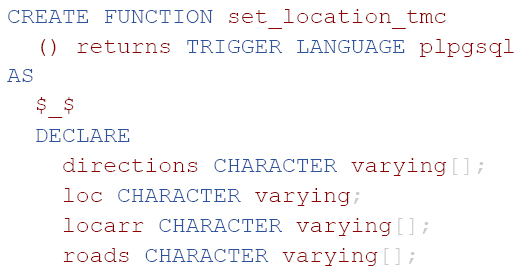
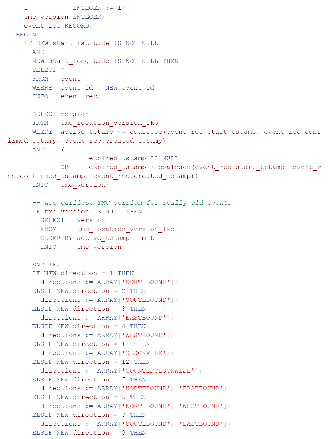
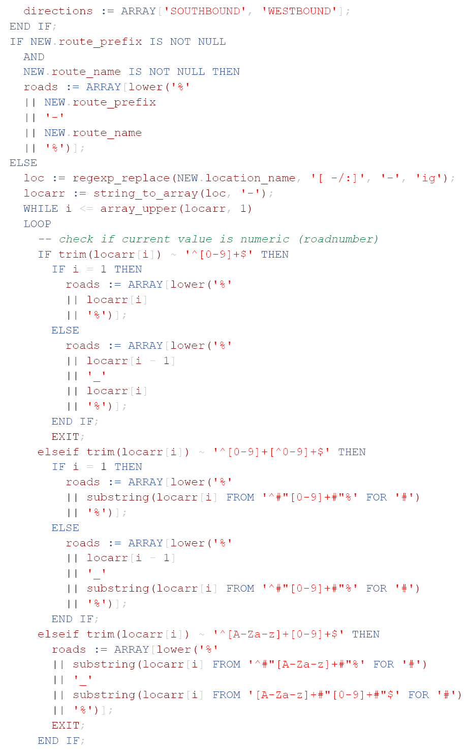
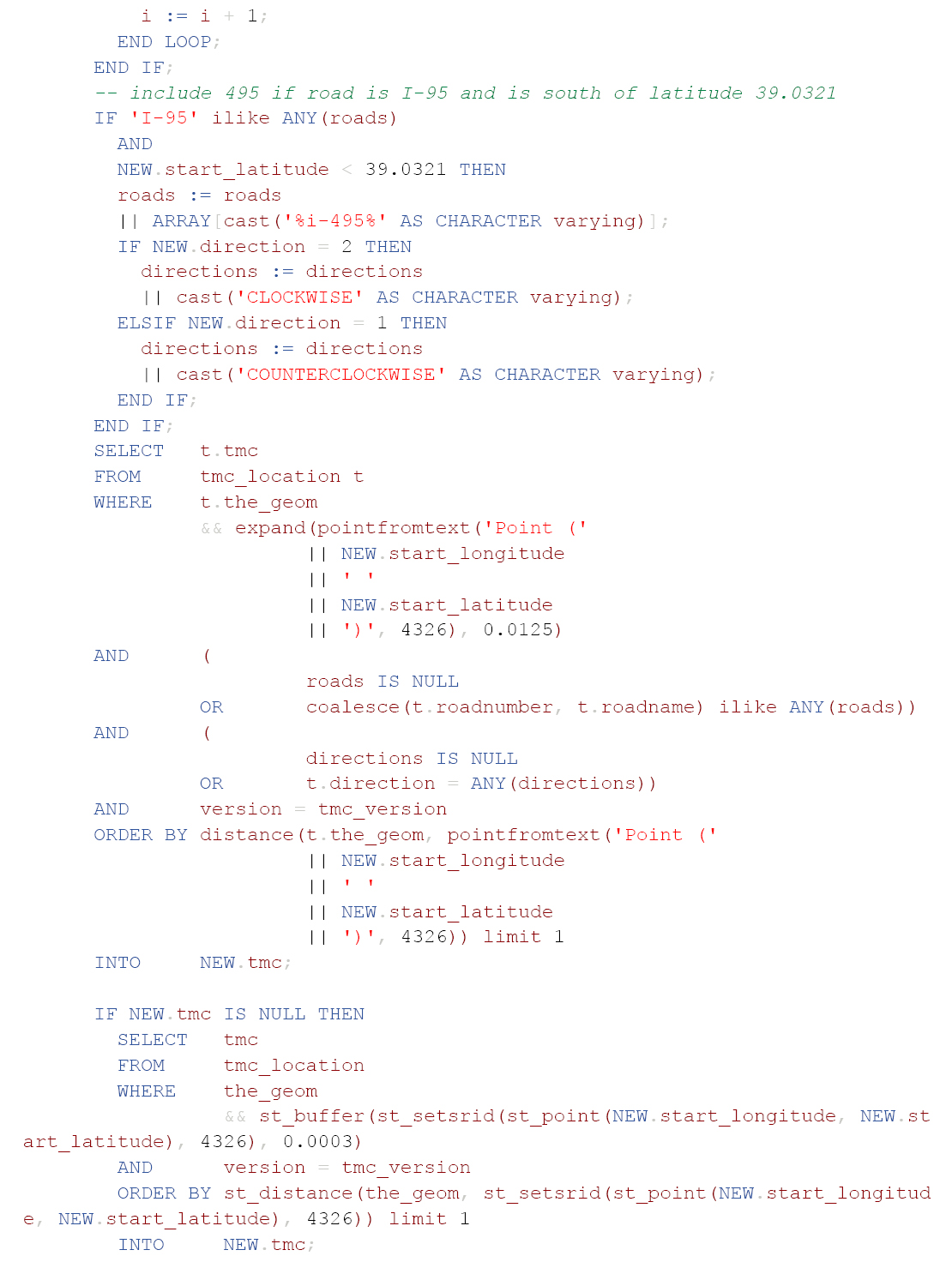
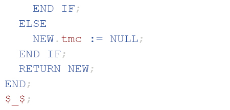
An example of SQL procedural language code for spatial alignment of CV event data with probe vehicle data before sending it on to Step #3 in the framework follows. This implementation conflates an incoming event to the TMC probe data segmentation. Depending on one’s preferred programming language and context of use, this code can be adapted and further developed to suit the requirements of a specific system or application.
5.3 Step #3: Region- and Use Case-Specific Fusion Algorithms
5.3.1 Executive Summary
In Step #1, the data were cleaned and prepared. In Step #2, different datasets were spatially and temporally linked. Those first two steps were simply preparing the data for their intended purpose. Here in Step #3, shown in Figure 14, additional algorithms are implemented that take the prepped and formatted data and turn it into useful information through any number of specialized fusion algorithms.

The fusion algorithm that is used for computing user delay will be vastly different from the algorithms used for predicting queues or estimating volumes. It is also important to know that there is no single “correct” algorithm for any use case. There are going to be dozens of different algorithms that could be implemented. No agency will have enough time or money to test every single algorithm to see which one is the best, and what is “best” for one agency may not be the best for another.
Some agencies may opt for simpler algorithms that are going to be easy to hand off and maintain over the long run, for example, extremely complex algorithms that can only be interpreted, modified, and maintained by highly specialized and expensive consultants or subject matter experts. Other agencies may opt for more complex algorithms—believing that they will produce more accurate or exact values for use cases that may mean life-or-death or require the best-of-the-best data. As mentioned earlier in this document, agencies will need to consider tradeoffs between complexity, quality, cost, and maintainability when implementing Step #3 of the data fusion framework, as this step can have the greatest impact on cost.
It is easy to be tempted by new technology and the excitement that ensues. Every agency wants to be able to state that they have the latest and greatest. But when it comes to data fusion, complexity can sometimes be the enemy. Agencies should be cautious of implementing the most complicated new AI and machine learning (ML) algorithms and ensure that they are actually the best tools for the agency’s use cases.
5.3.2 For the TSMO Professional
With advancements in AI and ML, new ways to fuse data are being developed each year. There are too many different fusion methods and algorithms to mention all of them in this report, and there is not necessarily one “correct” fusion methodology that will work with every use case, and each use case may have regionally specific data availability and other characteristics that might demand the use of one method over another. Below is a list of a few different types of algorithms that may be recommended or presented for evaluation. Understanding the basics of each fusion algorithm may be helpful in communicating with consultants or other implementation team members.
- Complementary Data Fusion: Complementary data fusion involves evaluating data from disparate sources or records that may be describing the same event in space and time (Castanedo 2013).
- Redundant Fusion: Unlike complementary data fusion, redundant fusion involves evaluation of disparate sources or records that describe the same components of the same event in space and time. For example, redundant data fusion may correlate traffic counts from a traffic sensor with number of trips from a probe vehicle routing dataset that represents every trip taken along the same roadway location where the sensor is located. This redundant information can be used to validate measurements or improve confidence in individual measurements.
- Cooperative Data Fusion: Cooperative fusion occurs when disparate data and information from different sources combine to produce new information. For example, a sensor may detect congestion in a particular location (due to drop in speed and increased sensor occupancy). At the same time, a probe-based routing dataset may show that vehicles approaching the congestion are rerouting to a parallel route to get around the congestion. The fusion of speed, volume, and occupancy data from the sensor and routing data can provide new information about travel behavior and real-time detouring.
- ML-based: There are many different ML models that can be leveraged for data fusion, but each is typically classified as follows.
- Supervised learning: Supervised learning establishes a relationship among independent variables (also known as “features” in ML) and a dependent variable (the predicted outcome—for example, travel time of a roadway segment). This relationship translates to a mathematical formula. The following three applications would typically use supervised learning techniques:
- Real-time short-term prediction.
- Network modeling.
- Data imputation/reconstruction.
Examples include multi-variate linear regression, multi-variate spatial-temporal auto-regressive moving average (MSTARMA), least absolute shrinkage and selection operator (LASSO), support vector regression (SVR), Kalman filtering, random forest, and deep learning.
- Self-supervised learning: This method is similar to supervised learning, but it does not rely on human annotated labels. In this case, the self-learning algorithm uses metadata or other information to automatically generate the necessary labels.
- Semi-supervised learning: This method is a combination of supervised and unsupervised learning in that it uses both labeled and unlabeled data to improve the performance of a supervised model. For example, semi-supervised learning can be used to infer traffic volumes by fusing two incomplete datasets, such as traffic sensors and vehicle trajectories (Meng, et al. 2017).
- Unsupervised learning: Analysts use unsupervised learning when the outcomes or labels (namely the dependent variable) are unknown or not defined explicitly, as opposed to the supervised learning. Unsupervised learning establishes a relationship directly among independent variables (also known as “features” in ML) without the observed labels. In general, unsupervised learning allows the understanding of typical patterns of a system based on
- Supervised learning: Supervised learning establishes a relationship among independent variables (also known as “features” in ML) and a dependent variable (the predicted outcome—for example, travel time of a roadway segment). This relationship translates to a mathematical formula. The following three applications would typically use supervised learning techniques:
For example, increased travel time along a segment captured by probe vehicles may indicate congestion, and the speed measurements from several sensors along that segment may also indicate congestion. While both sources of data are indicating congestion, the probe data describes that congestion based on a roadway segment and average travel time of multiple vehicles across the entire length of that roadway segment. On the other hand, point traffic sensors may detect various speeds at different locations along the segment providing a more granular understanding of congestion variations along that roadway segment. Similarly, sensor data may include per lane information that may provide insight in bimodal distribution of congestion that may not be evident from probe vehicle travel time data along a segment.
- Traffic pattern discovery.
- Traffic anomaly detection.
- Reinforcement learning: Reinforcement learning is a state-of-the-art ML technique that addresses the issue where supervised and unsupervised learning require a number of historical data in advance, and thus the cost of learning can be high and not adaptive to the real-time change in system dynamics of the built/natural environment. In reinforcement learning, an agent is defined to interact with the environment in real time, make an action (i.e., decision), and receive an observation (seen as a reward) to adaptively revise the optimal decision-making strategies. The agent learns from the environment by trial and error and is ultimately able to understand the system dynamics and make optimal decisions. Reinforcement learning can be value-based, policy-based, or model-based. Value-based reinforcement learning algorithms try to maximize the value function, while the policy-based algorithms try to define a policy (strategy for decisions) that maximizes reward in every state. Finally, model-based algorithms use virtual models created for each environment, and the agent performs in that specific modeled environment. Given that reinforcement learning is a decision-based process, it is often powered by Markov Decision Process and Q Learning models.
features without explicitly defining a specific outcome of learning or prediction. The following two applications would typically use unsupervised learning techniques:
Examples include K-means clustering, Gaussian Mixture Models (GMM), Density-Based Spatial Clustering of Applications with Noise (DBSCAN), Principal Component Analysis (PCA), and T-distributed Stochastic Neighborhood Embedding (TSNE).
Each of the listed methods has different algorithms and possible implementation strategies with varying pros and cons. Especially with AI and ML methodologies, implementers typically test several algorithms, train them, and then determine which is most accurate for the given scenario or use case. The implementation team may need to do the same. Last, note that it is rare that only one of the described methods will be used by itself. Instead, most use cases will employ multiple methods.
When working with an implementation team, give them time to collect enough data, test different algorithms, and be prepared to evaluate outcomes and make a go/no-go decision after seeing the results. For example, an attempt to predict queues on a facility that has dramatic seasonal variations in demand, incidents, etc., may require multiple years of data to properly train a more complex algorithm. While some algorithms can be implemented with less training data, the tradeoffs may be lower-quality results or results that change over time or algorithms that need frequent retraining or recalibration.
Larry Klein’s book, Sensor and Data Fusion for Intelligent Transportation Systems, provides additional examples of algorithms that may be relevant to the TSMO professional and region-specific implementation strategies. More information on this and other resources are found in Chapter 7.
5.3.3 Specific Implementation Guidelines
Unlike Step #1 and Step #2, Step #3 will likely be unique to the specific use case. For example, performing further data fusion for hurricane evacuation will be different from performing data fusion for sensor location optimization. First, the hurricane evacuation case will require near-real-time data fusion as well as consideration of data reliability given that sensor data may be impacted by environmental factors (such as visibility and precipitation), and probe vehicle data may be impacted by operational changes (such as counterflow) that will require re-interpretation of probe data readings to account for vehicles traveling opposite of segment direction definitions. On the other hand, the sensor location optimization use case is a planning use case that has a different time horizon and can utilize archived data at various levels of aggregation.
While these use cases are extreme examples, there can be distinct differences to data fusion approaches for “data quality improvements” and “volume data estimation.” And some use cases will have multiple viable fusion methodologies. For example, a rank-choice fusion methodology is incredibly simple with rules for when to select one dataset vs. another, but can still produce improved results for certain use cases. One agency that has implemented this methodology simply falls back on sensor data when the probe data supplier indicates a low level or reliability in provided data.
However, another agency has implemented a significantly more complicated ML algorithm for which significant training datasets, testing, and validation are required. The directions for implementing these two algorithms are significantly different and require different computational resources.
5.3.4 Examples of Implementation
The first example of an effective probe data and detector data fusion algorithm is Utah Department of Transportation’s (UDOT’s) use of a hybrid approach for traffic state estimation (Zhang and Yang 2021). The hybrid approach involves a combination of model-driven and data-driven estimation using ML.
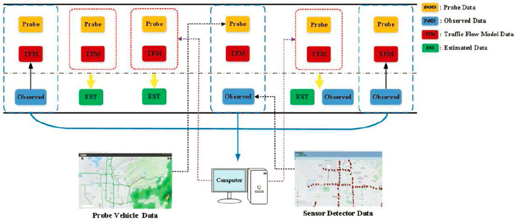
UDOT developed a pure ML approach that was shown to be ineffective with sensor data alone. Next, UDOT developed a pure ML with probe data approach which includes training of several ML models using observed probe and sensor data, followed by estimation of traffic state in location where there is no observed sensor data as shown in Figure 15. Observed sensor data and probe data are fed into a model to estimate speeds in locations where there are no sensor observations.
UDOT implemented this approach using the five regression models: SVM, random forest (RF), gradient boosting decision tree (GBDT), extreme gradient boosting (XGBoost), and artificial neural network (ANN). With addition of the probe data input, all five models resulted in estimates with acceptable accuracy as shown in Figure 16.
Given the potential for sparsity of probe data in the field, UDOT further enhanced the pure ML approach by developing a hybrid approach that introduces use of the second-order macroscopic traffic flow model (TFM) as an additional input value. First, the TFM is used to estimate the traffic state on each roadway segment using upstream and downstream detector data. Next,

Source: Zhang and Yang (2021)

Source: Zhang and Yang (2021)
the TFM results and probe data are combined to estimate the traffic state where no observed data is available as shown in Figure 17.
The pure ML approach performs better with some estimations, but this hybrid approach provides an alternative when probe speed data are sparse or unavailable.
A similar example of probe and detector data fusion to support traffic state prediction is outlined in Klein on pp. 70–71 describing two distinct approaches (2019): first, combining different datasets into a vector that is used as the input to the prediction model, and second using each dataset as a separate input into the prediction model followed by combination of model outputs to generate a prediction. This research has shown that different prediction models perform differently based on stability of conditions. For example, an ANN and classification and regression tree (CART) models predict general speed trend but fail to predict the fluctuation and are therefore not optimal for short-term prediction. On the other hand, SVR and kth nearest neighbor (KNN) can predict both trend and the fluctuation.
Another example of probe and detector data fusion application is in support of incident detection described in Ivan and Sethi (1998). This particular data fusion use case has been applied by many agencies for several years. The example fuses sensor data with probe data using discriminant analysis and a neural network to generate estimations of probability of an incident. If “anecdotal” data are available, they are fused with speed data to further enhance the estimation. One of the key challenges with incident detection using sensor and probe data fusion is potential for false positives. Both discriminant analysis and neural network analysis provide sufficiently low false alarm rates (< 0.18%) with high detection rate (87%) (Ivan and Sethi 1998).
PennDOT Voting Method
The Pennsylvania Department of Transportation (PennDOT) is one example of an agency that uses a more simple yet effective method of improving speed data quality by comparing probe data quality indicators to their own ITS point-sensor data. If there is a quality problem with one
Source: Zhang and Yang (2021)
data source (probe data), they simply select the speed data from the nearest ITS sensor and leverage it instead. The algorithm is relatively simple and somewhat similar to the “Voting Method” described in Klein (2019). As described in Klein’s book,
Voting methods combine detection and classification data from multiple sensors by treating each sensor’s declaration as a vote in which majority, plurality, or decision-tree rules are applied, often with the aid of Boolean algebra. Additional discrimination can be introduced via weighting of the sensor’s declaration if the sensor-system architect harbors doubts concerning a sensor’s reliability in specific environments or the independence of its output from that of other sensors. The voting technique is most effective when the sensors act independently of each other in providing outputs that signify the presence of an object or event of interest. The sensor outputs also contain information that expresses the sensor’s confidence that its declaration is correct and information concerning the object’s location. Detection modes consisting of combinations of declarations from two and three sensors have been proposed to provide robust performance in clutter, inclement weather, and environments where a particular sensor’s signature may be suppressed, e.g., by countermeasures in a military application. The detection modes utilize sensor confidence levels appropriate to the number of sensors in the detection mode. For example, the confidence levels for sensors in a two-sensor detection mode are typically greater than those in a three-sensor mode. A Boolean algebra–based voting algorithm can be derived to give closed-form expressions for the multiple-sensor system’s estimation of the object’s detection probability and false-alarm probability.
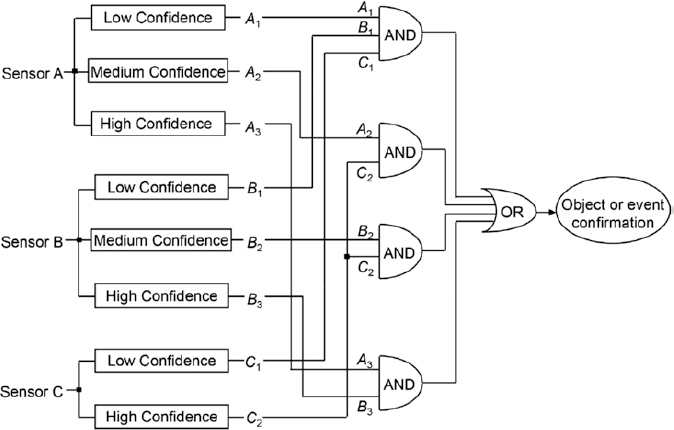
An example of a three-sensor system having four detection modes (A1B1C1, A2C2, B2C2, and A3B3) is shown in Fig. 2.13 [reproduced as Figure 18]. The three sensors are denoted by A, B, and C, and sensor confidence levels are denoted by subscripts 1, 2, and 3, where 1 represents the lowest confidence level of a sensor and 3 the highest. Only two- and three-sensor detection modes are considered in this example. The AND gates combine the sensor confidence level outputs corresponding to each detection mode of the system. The OR gate confirms an object or event detection by accepting the decision of the activated detection mode.
The difference in this method as described by Klein and the one employed by PennDOT is that instead of multiple “sensors,” there is weighted comparison between the confidence of point sensors and probe data. Those sensors or probe readings with the highest confidence are ultimately leveraged for the confirmation of the presence of congestion.

5.4 Step #4: Quality Control
5.4.1 Executive Summary
Quality control is where the work is checked and researchers make sure that the results for a specific use case are reasonable, accurate, and actionable (Figure 19).
But quality control is also not a one-and-done activity. ML models need training (which can be a part of quality control), but they often need to be retrained as time progresses and conditions on the roadway or driver behavior change. Even unsupervised systems usually cannot be automatically retrained automatically. The allure of generative AI and other ML is that they are somehow intelligent in ways that do not require supervision or human intervention. This is rarely, if ever, the case.
It is important not to rush the development team during this phase of the fusion. Allow them sufficient time to test and evaluate the results of their fusion algorithms. This can take weeks, months, and, in rare cases, years. And it is critically important to ensure that an agency’s long-term budget accounts for the maintenance of these systems—which is a part of quality control.
5.4.2 For the TSMO Professional
Quality control is an important step in the process of fusion of sensor and probe vehicle data as it provides a measure of confidence in both the process and implementation of that process. Each step of the process involves certain decisions and assumptions that may have compounding implications for the results. As such it is important to validate the results and adjust the process or implementation accordingly. Quality control results are used as feedback that guides adjustments to algorithms, inputs, and expectations. This framework feedback loop is an important component that ensures that the implemented algorithms are tuned to satisfy the specific goals and objectives of the fusion methodology.
The quality control step is not intended to achieve perfection, but rather to evaluate the quality of the results for a given use case and adjust input to the fusion process to achieve the desired level of quality. Each use case may have a different level of sensitivity which means that certain errors and assumptions may be satisfactory for one use case, but unacceptable for another.
There are several different ways to implement or apply quality control.
5.4.2.1 Validation with Ground Truth
If ground truth data are available, they can be invaluable in evaluating the results of the data fusion process. For example, if a data fusion application is used to detect incidents using fused sensor and probe vehicle data, then a CCTV stream could be used for ground truth validation. In other words, if the fusion algorithm detects an incident, an operator can view the live stream to verify that there is indeed an incident in that location at that time. Another example is validating the estimated speed for a location where ground truth speed data already exist. In this case it is important to define the acceptable level of accuracy for that estimation. This acceptable accuracy parameter can be defined based on the accuracy requirements as well as the “cost” of that accuracy. In other words, if the outcome of the speed estimation process is to be used in near-real-time operations, then that process must run fast enough to generate estimates in near real time. In that instance the accuracy to the nearest 5 mph may be sufficient as the difference between 65 mph and 60 mph on a highway may not be significant. However, if the estimated speed value is used for a collision avoidance application, then the level of precision and accuracy is a lot stricter. Iterative improvements and results that get one closer to reality or are indicative of trends may be perfectly acceptable depending on the use case.
The biggest challenge with ground truth validation is that ground truth is not always readily available. To be effective, ground truth data must be accurate, relevant, and timely. This sometimes requires deployment of temporary infrastructure to collect ground truth data, or procurement of a specific ground truth dataset.
5.4.2.2 Input Refinement
Data fusion algorithms may have varying degrees of sensitivity to their input data. For example, a lot of ML algorithms depend on high quality and high volume of training data to provide acceptable results. This means that the quality control process may result in an adjustment of input data quality parameters to ensure only higher-quality data are included, and addition of other data sources to reach the necessary volume of data needed to train the models. Similarly, results of a traditional model may indicate the need for additional calibration using real world data.
In addition to initial input refinement to achieve desired results, all models require continuous maintenance, retraining, and calibration. By their very nature, models are a snapshot of a real-world process. These processes are dynamic and change (at various speeds), causing “drift” that eventually makes the initial model snapshot no longer representative of the real-world process. Even so-called self-training and self-learning models may require maintenance to account for changing conditions, loss of data, environmental factors, or to adjust for changing agency goals.
5.4.2.3 Model Adjustments
During the quality control process, in addition to adjusting input data for models, the actual models may need to be modified to address results quality. For example, it is important to tune a ML model’s hyperparameters until desired results are reached. Hyperparameters control the model structure, function, and performance, and the exact settings for those hyperparameters may not be evident or straightforward. As part of quality control, hyperparameters can be tuned and results re-evaluated until optimal hyperparameter values are discovered. Similarly, adjusting clusters may have meaningful implications for results of a model. For example, density-based clustering methods may create results that are very different from hierarchical-based clustering methods.
In addition to adjusting the mechanics of the model, sometimes the quality control process indicates the need to adjust overall assumptions and data fusion targets. For example, initial model accuracy targets may prove to be overly aggressive, resulting in models and processes that continue to fail to meet the desired goals. Reassessing targets may expose opportunities to achieve acceptable goals using more conservative targets. Similarly, data fusion process results may expose unexpected outcomes that require revisiting and adjustment of the initial assumptions.
5.4.2.4 Manual Quality Control
While quality control automation is important to ensure repeatability and continuous validation, manual quality control has an important role in identifying potential issues that may only be discoverable by human interpretation of data and environmental conditions. For example, a quality control specialist may be able to identify issues related to environmental factors such as areas with bad reception, mountains, urban canyons, tunnels, reversible lanes, express and non-local lanes, new facilities, and so on.
5.4.2.5 Quality Control Documentation
Quality control process outcomes and actions must be documented to provide traceability for the data fusion methodology adjustments to enable future process guidance and input. This documentation can include methodology adjustments, data properties and tagging considerations, assumptions and targets, and associated code or procedures.
5.4.3 Specific Implementation Guidelines
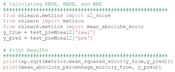
The quality control process may include evaluation of common statistical indicators to determine how well a particular model or algorithm is performing. Common statistical indicators include root mean square error (RMSE), MAE, mean absolute percentage error (MAPE), and others.
RMSE is the square root of the average of the squared difference between the observed value (yi) and a value predicted by a regression model (). This error shows how far predictions fall from measured true value using Euclidean distance (Bajaj 2023).
MAE is the average of the difference between the ground truth (yi) and the predicted values (). This measure captures how far the predictions were from the actual output, but does not provide information about the direction of the error, making it difficult to discern if the model is underpredicting or overpredicting (C3.ai n.d.).
MAPE is a mean of absolute relative errors representing how far off predictions are on average.
The quality control process includes setting acceptable values for these various statistical indicators and evaluating results against those target values.
For example, UDOT’s traffic state estimation use case applies these three statistical indicators to evaluate various machine learning model outputs and output changes with changes to the model definition and input data (Zhang and Yang 2021).
5.4.4 Examples of Implementation (Zhang and Yang 2021)