Data Fusion of Probe and Point Sensor Data: A Guide (2024)
Chapter: 6 Real-World Implementation Examples
CHAPTER 6
Real-World Implementation Examples
To illustrate the real-world application of this data fusion framework, here are two use cases:
- Utah DOTs fusion of point sensor speed data and probe data to create a more accurate statewide speed dataset (Zhang and Yang 2021).
- The CATT Lab’s use of volume data from point sensors fused with probe-based speed data for computing user delay and then further fusing incident data from CVs and other sources to identify the causes of congestion on roadways (Franz, Pack, et al. 2022).
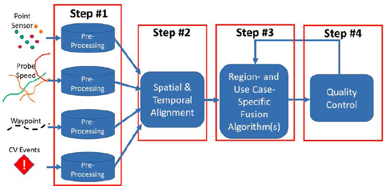
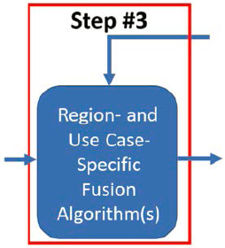
Both use cases showcase data fusion of probe and point-sensor data. While both follow the broad data fusion framework steps as described in this report, both implement their own, unique use case-specific fusion algorithms as shown in Step #3 of the framework (Figure 20).
For example, Utah DOT implements a set of ML algorithms in Step #3, and the CATT Lab implements a cooperative data fusion algorithm. This Section of the report highlights those differences during a detailed explanation of how these two agencies approached data fusion. For each use case, the following information is provided:
- Purpose of the use case
- Data sources
- Data fusion framework steps that the use case implemented
6.1 UDOT Speed Data Quality Improvement Use Case
The first use case is from Utah DOT and researchers Xianfeng Terry Yang, Zhao Zhang, and Brian Azin. The following information is heavily referenced in Utah DOT reports UT-20.15 and UT-21.03. The research team for this paper thanks the authors of the Utah DOT reports for their permission to present their work and reprint images and code.
6.1.1 Purpose
UDOT has access to agency-installed point-sensor data that reports speed data. The agency also procures probe-based speed data from the private sector. At the time of development of this research project, UDOT determined that generally, point-sensor data provided more accurate speed measurements than probe data due to the probe data being biased. Probe data bias is a result of low penetration rate of probe data (around 2% of total traffic, according to the UDOT use case researchers in March 2021). The bias is based on the type of vehicles which are capable of reporting their GPS location and their geographic distribution, as well as length of the segments on which data are reported. Figure 21 shows how the length of segments on which data are reported results in probe data speeds remaining unchanged over the length of those segments, while the sensors within those segments indicate variations in speed between individual locations.
However, UDOT also realized that ubiquitous probe data coverage allows for statewide monitoring that is not possible using only the point sensors.
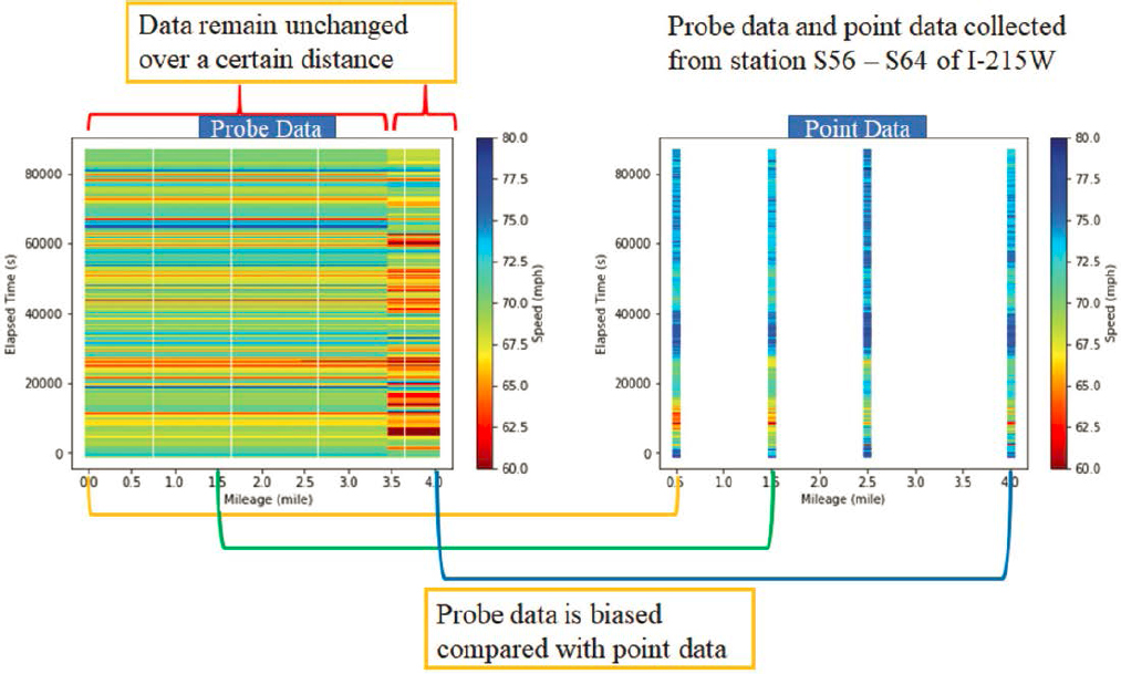
Source: Zhang and Yang 2021
To address this challenge, UDOT developed a methodology to process their point-sensor data and fuse it with probe vehicle data using a set of machine learning models to produce a more reliable estimate of statewide traffic speed and flow patterns.
6.1.2 Data Sources
The data used in the fusion process came from two sources:
- Point-sensor data stored in the UDOT Performance Measurement System (PeMS) platform.
- Probe-based speed data stored in the ClearGuide platform.
The UDOT PeMS platform collects point-sensor data consisting of vehicle counts and occupancy in 20-second intervals. Using these two variables, the system then calculates the speed at that location and aggregates the measurements to 5-minute intervals for use in operations.
The ClearGuide platform stores and makes available third party-provided statewide 5-minute probe speed data which is used in operations, specifically in locations that lack point sensors.
6.1.3 Data Fusion Framework Steps
6.1.3.1 Pre-Processing
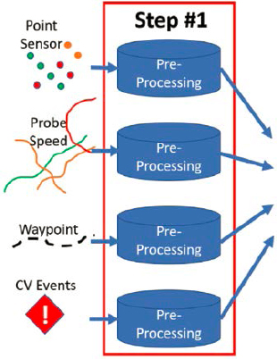
Prior to data fusion, UDOT performs a set of rigorous cleaning steps to ensure the highest possible quality of sensor data to be used in the ML algorithms. While ML models are good at capturing the stochastic nature of traffic data, they depend heavily on quality and quantity of training data. This step is important because poor quality or sparse training data will severely degrade the performance of the ML algorithm (Figure 22).
Physical sensor devices may become unreliable in reporting accurate data due to lack of maintenance and calibration, or due to field communications issues. The initial screening step uses
the basic traffic flow characteristics and traffic flow conservation to detect the most obvious data errors. UDOT identified four types of errors in their sensor data:
- Missing data
- Data with large variations
- Out-of-range data
- Data inconsistencies
Missing Data
Data can be missing from the database due to a few different reasons. First, there could be short-term gaps that are caused by insufficient information due to flow rates or due to intermittent issues with field communications. Second, there could be extended periods of time where data are missing due to a faulty sensor that does not report data or due to a communication loss to that field device.
Data with Large Variations
This error occurs when two adjacent sensors report large variations in traffic flow between them that cannot be accounted for in changes on the road segment between them. In other words, this occurs when traffic flow changes between two adjacent sensors are physically impossible due to the basic traffic flow theory and traffic flow conservation. While large variations between adjacent sensors indicate an error, adjacent lane variations may be normal due to the uneven distribution of vehicles between lanes. For example, trucks often occupy right lanes in a higher volume than left lanes.
Out-of-Range Data
The Highway Capacity Manual (HCM) specifies minimum and maximum values for flow, speed, and occupancy based on road characteristics in addition to the sensor data checks shown in Section 5.1.3.1. “Out-of-range data” are measurements that fall below the minimum values or above the maximum values.
Data Inconsistencies
UDOT determined that there could be data inconsistencies between raw data collected by the field devices and the aggregated value available in the PeMS database. For example, PeMS collects vehicle counts and occupancy in 20-second intervals, and then calculates speed based on those metrics and aggregates all those values into a 5-minute interval record. If there are any errors that occur during this calculation and/or aggregation process, there will be data inconsistencies between raw data and processed data.
The pre-processing algorithm first looks for missing data and irregular recorded parameters, followed by a two-stage examination of the distribution of average effective vehicle length (AEVL).
Primary Screening
The primary screening step examines every sensor station for missing variables. If some of the expected metrics (speed, volume, or occupancy) are missing, then that data for that time period from that sensor are considered missing. If data for all variables are present, then a single variable threshold check is performed to verify meaningful ranges, mainly:
- Flow in veh/lane/hr (qi): 0 ≤ qi ≤ qmax
- Speed in mph (vi): 0 ≤ vi ≤ vmax
- Occupancy as % of occupancy (oi): 0 ≤ oi ≤ omax
If any of the three metrics is zero, then the other two metrics must be zero. If the data record fails any one of these checks, the record is discarded for the purpose of further analysis.
Piecewise Quality Check
After the records that failed the primary screening are removed, the pre-processing algorithm evaluates the remaining data using the detector AEVL distribution and Kolmogorov-Smirnov (KS) test to uncover erroneous records. The AEVL is defined as:
and AEVL distribution of a detector is measured over a specified time interval (e.g., 1 hour). This distribution is then compared to the AEVL distribution of upstream and downstream sensors. The K-S test evaluates the likelihood of these two sample distributions being drawn from the same probability distribution. In other words, the K-S test determines whether the AEVL of the examined sensor statistically makes sense in context of its upstream and downstream neighbors. If the AEVL distributions are statistically different, the resulting difference provides insight in changes in data patterns to flag erroneous records.
Continuous Quality Check
The next check uses multiple comparisons with the best (MCB) method to identify potential bad records not captured by previous checks. The key feature of the MCB method is that it compares AEVL of each lane of traffic at neighboring stations and uses the calculated confidence interval (CI) for statistical assessment. This method requires data collected over a sufficiently long period of time (e.g., 1 week) so that data can be grouped into equal segments (e.g., 1 hour) and the mean and variance of the group can be computed. If the CI contains zero, that indicates that there is no significant difference of AEVL at neighboring stations.
UDOT determined three possible outcomes based on the results of the piecewise quality check and continuous quality check:
- If sensors show no significant errors in both steps, there is a 95% CI that no other error is present.
- If the target sensor shows no errors during the continuous comparison check but does indicate some in the piecewise check, it can be concluded that there might be a change in traffic flow patterns such as a special event, or there might be a fixed error within the detector.
- If the sensor only fails the continuous comparison check, an additional investigation is needed due to two possible scenarios: a) the target sensor may have an error, or b) the adjacent station sensor may not be in proper working order.
If a sensor is found to be faulty during the additional investigation, it is excluded from further quality checks, and the next nearest sensor is used instead.
Example Results from UDOT Implementation Case
This pre-processing algorithm of Figure 23 was applied to an example case to demonstrate the results. The researchers evaluated sensor data on I-15 northbound from January 12, 2019, to January 19, 2019. Note that the UDOT use case implementers use the term “detector” in Figure 23 in the same way the term “sensor” is used in this report.
The demonstration area included 61 sensors across roughly 9.5 miles of I-15 (between mileposts 302.75 and 312.16) as shown in Figure 24.

The single variable thresholds were set as follows:
- Flow: 180 vehs/5 mins/lane
- Speed: 90 mph
- Occupancy: 95%
The results were as follows (Figure 25). Note that the percentages don’t add up to 100% as errors can occur multiple times throughout different stages of the algorithm.
- No error: 85.41%
- Missing data: 10.46%
- Primary error: 1.39%
- Piecewise comparison: 3.62%
- Continuous comparison: 2.74%
The results showed some variation in error rates based on sensor location (e.g., ramp vs. mainline vs. HOV) as shown in Figure 26.

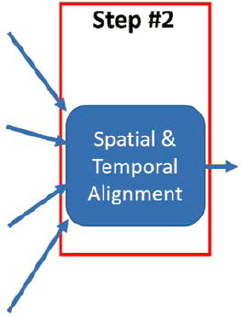
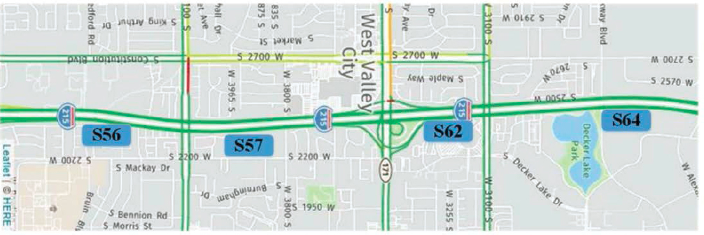
6.1.3.2 Spatial and Temporal Alignment
In this step, the pre-processed sensor data from PeMS are temporally and spatially aligned with probe speed data from ClearGuide (Figure 27). Mainly, the study identified a set of sensors along the corridor and corresponding probe data segments between the first and last detector as shown in Figure 28. The probe data are reported on roadway segments defined using the TMC standard. The latitude and longitude of each sensor is compared to the start and end points of TMC segments along the corridor to identify an appropriate TMC segment that sensor belongs to. Both sensor speed and flow, and probe speed data are reported in 5-minute intervals over the study time period (14 days). For each matching 5-minute interval, a record for a sensor and corresponding TMC segment is captured for a total of 4,032 records for each sensor and TMC segment.
Depending on further use case needs for the pre-processed sensor data, additional steps may be taken. In the case of UDOT’s sensor and probe speed data fusion using ML algorithms, the final pre-processing step includes normalization of raw speed and flow data. This normalization is necessary because of the sufficiently different scales for the two metrics. Normalization allows


Source: Azin and Yang (2020)
raw speed and flow data to be constrained to the range from 0 to 1. The normalization equation is as follows:
where xn is normalized speed and flow data, xi is raw speed and flow data, and xmax and xmin are the maximum and minimum values of raw speed and flow data, respectively.
6.1.3.3 Use Case-Specific Fusion Algorithm
The UDOT use case is estimating traffic state by training a set of ML algorithms using integrated sensor and probe data (Figure 29). In other words, observed sensor and probe speed data
Source: Zhang and Yang (2021)
are inputs to a model that estimates the traffic state in locations where sensor data are not available. Unlike the traditional TFMs that are developed based on a strong assumption that does not accommodate data uncertainties, ML is able to capture the stochastic nature of data. This use case applies two approaches for traffic state estimation: a pure ML approach and a hybrid ML approach. The key difference between these two approaches is that the pure ML approach relies purely on sensor and probe data to train the ML algorithm, while the hybrid ML approach introduces the second-order macroscopic traffic flow model as an additional training variable grouped with sensor and probe data.
Pure Machine Learning Approach
The pure ML approach uses four steps:
- Step #1: For a freeway segment, i, with probe data only, select the upstream and downstream stations that have both probe and observed data available for model training.
- Step #2: Train ML models (e.g., SVM, RF, GBDT, XGBoost, and ANN) at both upstream and downstream stations, based on the grouped dataset.
- Step #3: Use the two trained models to estimate the traffic state for freeway segment i, and select the one with better performance (e.g., lower RMSE).
- Step #4: Repeat Steps #1–3 until all freeway segments without observed data are studied.
UDOT uses several ML algorithms and measures their performance to select the best algorithm for each case.
The SVM algorithm is a supervised model that can be used in a wide variety of applications including regression and prediction. The RF algorithm uses a multitude of decision trees during training to generate predictions that can be averaged for each tree and returned as a result. The GBDT is an algorithm that relies on boosting weak prediction models such as simple decision trees into a one strong prediction. The XGBoost algorithm is a software library that implements a more regularized form of gradient boosting that performs very fast and tends to be better at model generalization. Finally, an ANN uses a connected network of artificial neurons (nodes) that communicate to each other based on the input values and activation functions. ANNs typically contain an input layer, a number of hidden layers, and an output layer, where each layer groups nodes performing a particular type of transformation.
The performance of each of these algorithms can be measured using various statistical indicators. UDOT researchers used RMSE, MAPE, and MAE to evaluate the accuracy of the estimated traffic speed and flow.
The UDOT team implemented the pure ML approach along a two-and-a-half-mile stretch of the I-215 corridor in Salt Lake City, UT. They collected 2 weeks of sensor and probe data from January 7, 2019, to January 20, 2019, and tested all trained models at a location where they had observed sensor data to evaluate accuracy of the estimated values.
The initial implementation did not use probe data as input, and as a result all models performed poorly with all statistical indicators at an unacceptable level:
- Flow indicators:
- RMSEs > 69 veh/5-min
- MAPEs > 50%
- MAEs > 41 veh/5-min
- Speed indicators:
- RMSEs > 3.35 mph
- MAPEs > 2.6%
- MAEs > 1.8 mph
Figure 30 shows the performance of pure ML algorithms without probe data. The observed flow and speed are not accurately reflected by the pure ML algorithms without probe data, failing to capture the variations in observed values.
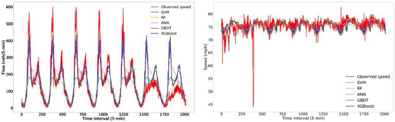
The next implementation included probe data as an additional input. All models performed significantly better than without probe data, resulting in the following statistical indicator values:
- Worst-case flow indicators:
- RMSE = 36.26 veh/5-min
- MAPE = 35.16%
- MAE = 26.28 veh/5-min
- Worst-case speed indicators:
- RMSE = 3 mph
- MAPE = 3.03%
- MAE = 2.2 mph
Figure 31 shows the performance of pure ML algorithms with introduction of probe data. In this case the observed flow and speed values and their variations are more accurately captured by the pure ML algorithms with probe data input.
Source: Zhang and Yang (2021)

Source: Zhang and Yang (2021)
Hybrid ML Approach
The accuracy of ML models depends heavily on the quality and quantity of training data. If training data are noisy or small, the performance of the ML algorithms may not be acceptable. The hybrid ML approach is intended to provide an alternative input data in cases where probe data are not available. In other words, this approach addresses the issue of the low performance of the pure ML models without probe data by introducing an alternative input dataset that can enable estimation in locations where there is no observed sensor and no observed probe data. The alternative input data are generated using the second-order macroscopic TFM. This model uses observed flow and speed at upstream and downstream stations, on-ramps, and off-ramps to estimate the traffic speed evolution on the target freeway section.
The hybrid ML approach then uses the observed sensor data, the second-order macroscopic TFM estimates, and observed probe data if they are available as training inputs into previously described ML algorithms.
The UDOT research team implemented the hybrid ML approach using the same dataset and parameters as what they used in the pure ML implementation. The results indicate that the pure ML implementation with probe data performs better than the hybrid ML approach. However, the performance of the two approaches is close, and the hybrid ML approach compared to the ground truth indicates that this approach could be used to accurately estimate flow and speed in the absence of probe data.
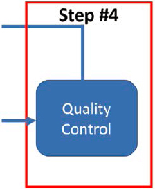
6.1.3.4 Quality Control
The accuracy of ML models depends heavily on the quality and quantity of training data (Figure 32). If training data are noisy or small, the performance of the ML algorithms may not be acceptable. This means that care must be taken when gathering and preparing training data to ensure that a sufficient volume of high-quality data are available.
However, even with the same volume and quality of data, various ML algorithms perform differently. The key is to evaluate outputs and select appropriate ML models and adjust them accordingly.
For example, in the UDOT use case implementation, each ML model’s performance, according to the statistical indicators, varies based on input data and can perform well for certain metrics in comparison to other models. Table 6 summarizes the performance of various ML models implemented in the UDOT use case. First, the relatively low values of TFM data’s RMSE, MAPE, and MAE show that TFM data could be a potential replacement of probe data when developing ML models for TSE. The yellow highlighted values in Table 6 show the performance of hybrid models, while the blue highlighted values show the performance of hybrid models with probe data indicating a generally better performance when probe data are used in the hybrid model.
The performance of models is also highly dependent on the location. In general, a well-performing model may only be applicable to nearby locations and may not be transferable to other freeway segments. This means that outputs must be verified, and the model adjusted accordingly as the model is implemented in various locations.
Finally, ML models may need to be retrained when the original data become dated. This means that, to maintain accuracy of estimates, the maintenance of these models must be a continuous effort.
6.1.4 Lessons Learned and More Information/Details
As was described in Chapter 4, not all fusion methods and use cases may yield results that warrant the investment. The Utah DOT example, when compared to the PennDOT use case
Table 6. Comparison of performance of each ML model.
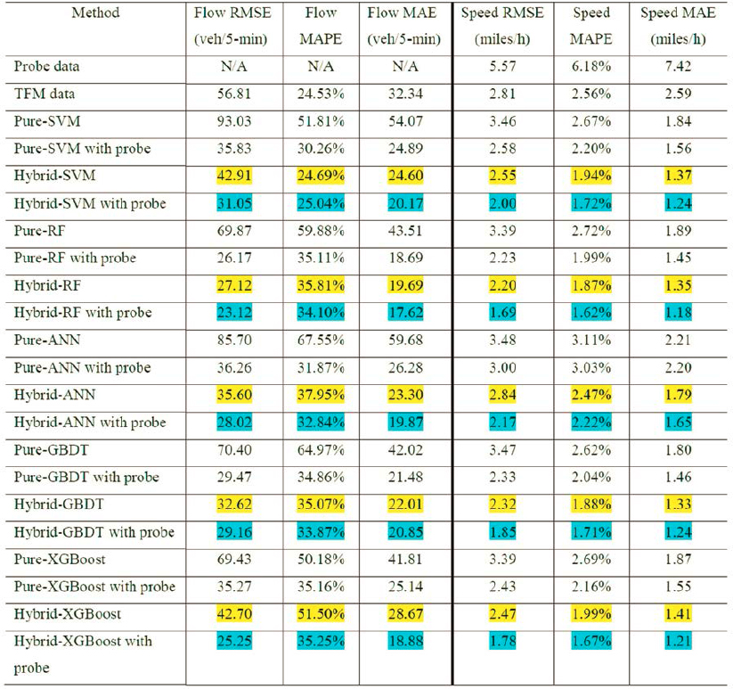
Source: Zhang and Yang (2021)
described in Chapter 5, is significantly more sophisticated and complex, and leverages the latest in ML technologies. However, complexity alone cannot always guarantee high-quality results, especially in situations where data are sparse or location-specific algorithms may be required. ML and AI may not always be the best solution to every data problem. That said, the algorithms employed in this use case may be relevant to other DOTs and other situations. They also follow a logical approach to data fusion.
This use case was developed for Utah DOT by researchers Dr. Bahar Azin, Dr. Zhao Zhang, and Dr. Xianfeng Terry Yang, with graphics and text reprinted with their permission. The two research reports from which the bulk of the material from this use case was derived can be found at https://site.utah.gov/connect/about-us/technology-innovation/research-innovation-division/ and include:
- Azin, B., and X. T. Yang. (2020). Multi-Stage Algorithm for Detection-Error Identification and Data Screening. Report No. UT-20.15. Utah DOT, Taylorsville, UT.
- Zhang, Z., and X. T. Yang. (2021).Utilizing Machine Learning to Cross-Check Traffic Data and Understand Urban Mobility. Report No. UT-21.03. Utah DOT, Taylorsville, UT.
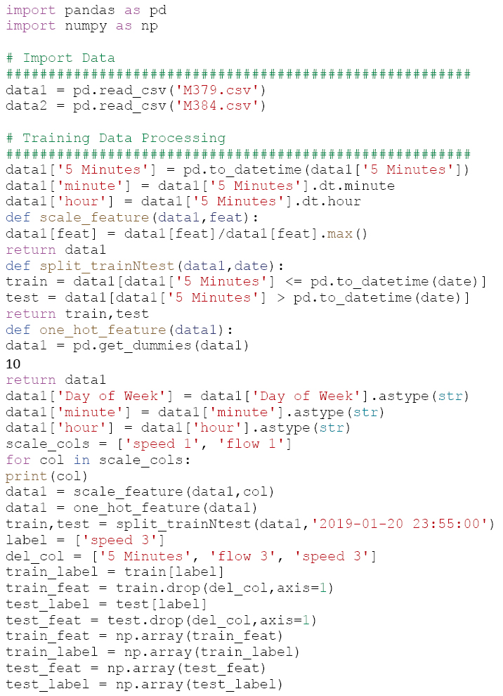
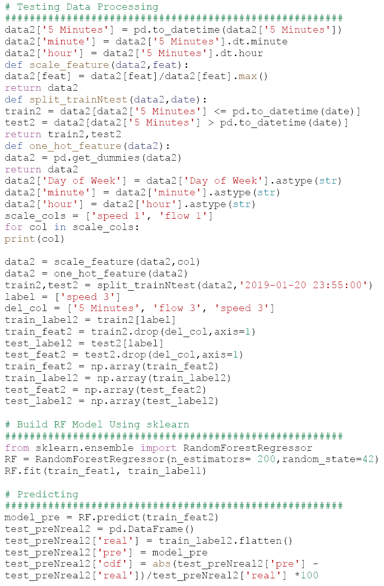
6.1.4.1 Example Implementation Code for the Continuous Model
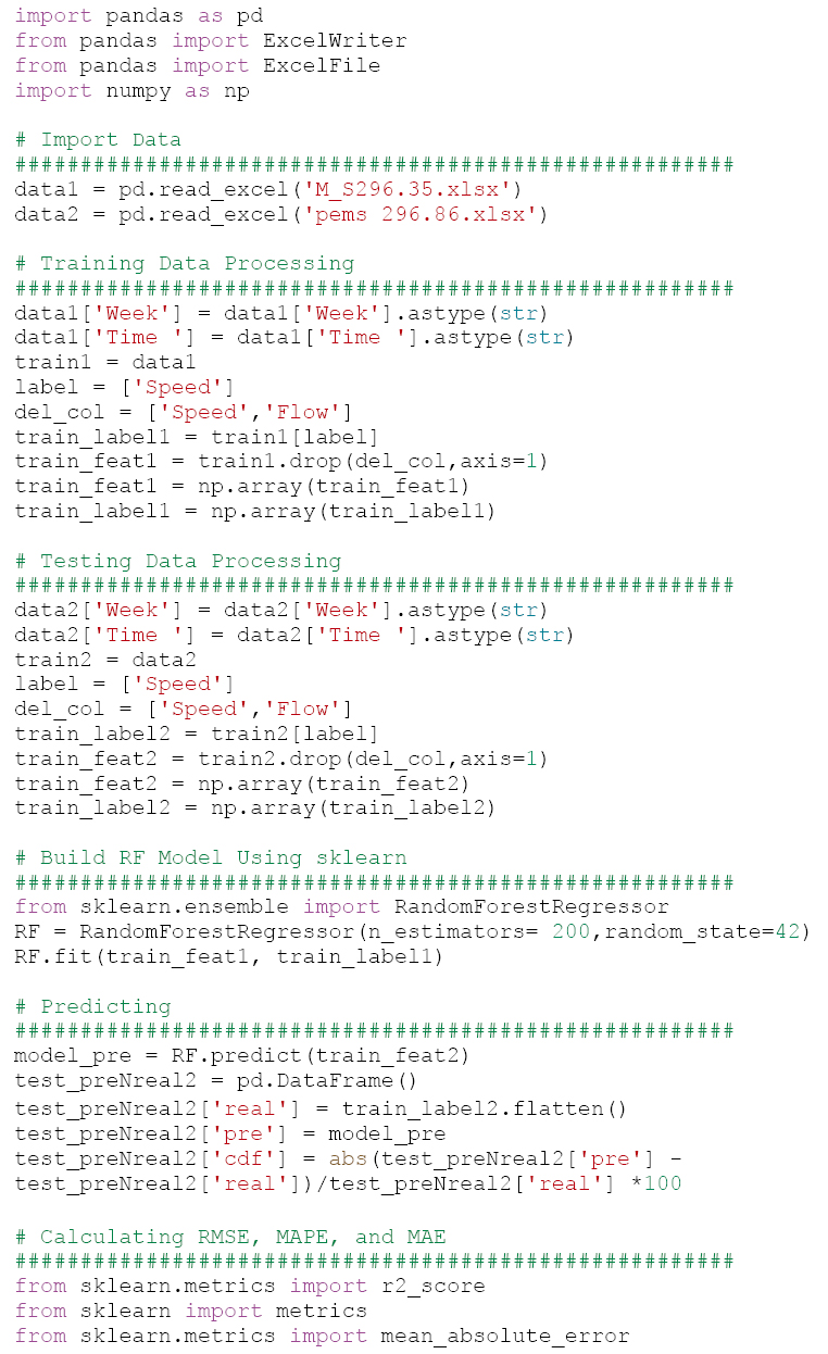
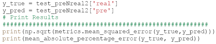
6.1.4.2 Example Implementation Code for RF Model
6.2 CATT Lab User Delay Cost and Causes of Congestion Fusion Use Case
The second use case comes from the University of Maryland CATT Laboratory. Special thanks are extended to their research team for sharing their research papers and presentations in support of this publication.
6.2.1 Purpose
The CATT Laboratory, in collaboration with the Bureau of Transportation Statistics, TETC, and a nation-wide group of transportation engineers from 35 state DOTs, nine metropolitan planning organizations (MPOs), and two universities, developed a data fusion methodology whose initial purpose was to rebuild the 2004 national Congestion Pie Chart, shown in Figure 33. This original pie chart, while innovative at the time, was largely built off modeled data and was a single pie chart that represented the entire country (Cambridge Systematics and TTI 2004).
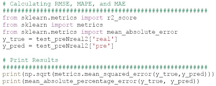
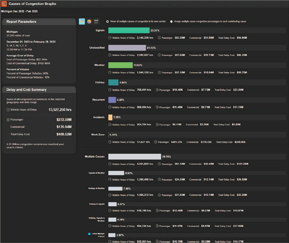
By 2019, it was realized that there were now real-world data that would allow the research team to develop a new congestion pie chart that would not need to rely on modeled data and would be able to compute the causes of congestion in every county of every state in the country—showing local causes. The result was a revised Causes of Congestion Pie Chart for the National Highway System that showed different results and provided new categories of congestion including

Source: Cambridge Systematics and TTI (2004)
“multiple causes” where the combination of two or more causes was included as depicted in Figure 34. For example, a crash occurring in a work zone or a crash occurring during a snowstorm would be combined into two multi-cause categories.
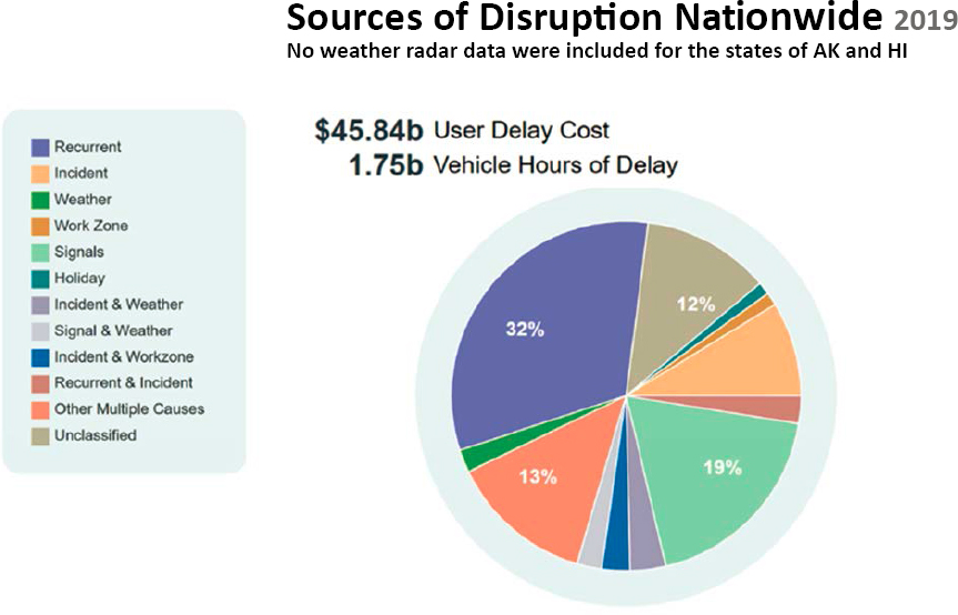
The original methodology, as described in ITS America Paper 1189052 (Franz, Tous, et al. 2022), leveraged probe-based speed data, volume data from point sensors, crowdsourced event data, and other sources. The high-level steps for computing the causes of congestion are shown in Figure 35.
The CATT Laboratory then expanded the original methodology to include all roads covered by probe data, and expanded the incident and event data sources to be able to include agency-provided work zones, ATMS events, police crash datasets, and most notably event data from CVs. The new system lets users select individual corridors (from any starting point to any ending point), multiple corridors, ZIP codes, counties, groups of counties, an entire state, group of states, or specific functional classes of roadways in any geography before computing the causes of congestion. There are no date restrictions on the search functionality so long as the underlying data (probes, events, volumes, etc.) are available. Some states have nearly a decade of data available. The results are more granular, too, giving results that encompass every possible combination of multiple causes.
6.2.2 Data Sources
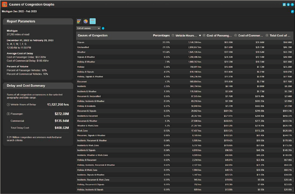
The initial analysis focused on the National Highway System only, but the current analytics as shown in Figures 36 and 37 include any road segment that is covered by private-sector probe
Source: University of Maryland CATT Laboratory
Source: University of Maryland CATT Laboratory
data providers. The only caveat is that there must also be readily available traffic volume data from point sensors conflated to the same network as is used to report probe data. Other data sources that are used to derive cause are shown in Table 7.
This analysis required the fusion of all of these datasets in iterative pre-processing steps. Additional computations not related to data fusion may not be covered fully in this report.
6.2.3 Data Fusion Framework Steps
This use case is complex in that it requires the fusion of many disparate data sources, not just point and probe data. The first step is the fusion of the point-sensor volume data with probe-based speed data to compute user delay. After that, this paper will explain the fusion of other point and probe data sources, such as probe-based event data from CVs. Less focus will be given to the fusion of other data sources, like those from weather data sources to roadway segments.
6.2.3.1 Pre-Processing
The pre-processing (Figure 38) for this use case required several cleaning and formatting steps including the following per each data type, as shown in Table 8.
The CATT Lab is not directly creating the probe-based speed data or the conflated volume datasets. They are simply provided to the Lab by third parties. The CATT Lab then checks these two datasets for completeness or gaps. With probe-based speed data, completeness refers to temporal gaps in data coverage and spatial gaps in coverage. Spatial gaps are exceedingly rare, but they do occasionally occur with some data providers. It is more common for temporal gaps to occur than spatial gaps. The probe data are used regardless of confidence or other quality indicators as it has been shown that it is rare to have congestion and low-confidence data at the same
Source: University of Maryland CATT Laboratory
Source: University of Maryland CATT Laboratory
Table 7. Causes of congestion data sources and size.
| Data Item | Data Source(s) |
|---|---|
| Congestion | 1-minute probe-based speed data |
| Incidents/Events/Work Zones | Connected vehicle event data, crowdsourced event data from Waze, ATMS events, police crash reports, Work Zone Data Exchange (WZDX), lane closure permitting systems, etc. |
| Weather | National Oceanic and Atmospheric Administration (NOAA) radar and Waze |
| Holiday Travel | Holiday Calendars (including travel days before and after holidays) |
| Signals | OpenStreetMaps (OSM) Traffic Signal Databases and Agency-provided Signal Location Databases |

time. If low-confidence data are presented, it is usually during uncongested times that would not impact the results of this use case.
Similarly, with the volume datasets, the CATT Lab is concerned with both temporal and spatial gaps. By the time volume data are delivered to the Lab, conflation to the TMC road network has already occurred. The Lab is simply looking for the absence of volume data for any TMC segment. If volumes do not exist for certain segments, the data providers are notified, and volume data are provided in a redelivery. There is no checking of the quality or accuracy of the volume data, as that is done by the agency and private sector prior to submission to the CATT Lab.
With respect to incident and event data from agencies, police crash reports, Waze, and CVs (probes), the CATT Lab is only performing high-level checks for unreasonable gaps that could be an indicator of a loss of a particular data feed. For example, the Lab may create basic metrics surrounding the typical number of incidents, work zones, etc. that should be seen on any given day. If a day or region is significantly out-of-range—especially when numbers go to zero for long periods of time, then time ranges are flagged, and systems administers are notified so that any gaps can be addressed.
Duplicates may also be removed if they exist. To identify duplicates, a dual search for incidents within the ± 0.4-mile radius that occurs within 30 minutes of one another is conducted
Table 8. Pre-processing for causes of congestion use case.
| Data Type | Pre-Processing Steps |
|---|---|
| Probe-Based Speed Data | Speed data are checked for completeness and availability. If significant gaps are detected that could impact results, the data provider is contacted for backfill. |
| Volume Data from Point | Volume data are collected from point detectors by third parties (agencies and/or the private sector) and then conflated to TMC segments by the same third party. |
| Detector | The CATT Lab receives these datasets and checks for completeness. |
| Weather Data | See Step #2 on spatial fusion. |
| Events | Check for gaps or other inconsistencies and add TMC segment as a location variable (see Step #2). |
(Pack 2017). Incidents matching these criteria may be grouped together as the same incident. This same methodology is modified for regional variations. For example, the 0.4-mile radius may be appropriate for rural areas, but may need to be shrunk for urban areas where more incidents within a short distance may be more likely to occur.
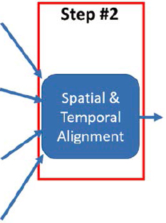
6.2.3.2 Spatial and Temporal Alignment
This use case required the spatial and temporal alignment of multiple datasets (Figure 39), including:
- Fusion of volume data from point sensors with probe-based speed data
- Fusion of events and incidents to roadway segments
- Fusing of NOAA radar and RWIS data to all roadway segments
- Fusion of signals to roadway segments
Volume data were delivered to the CATT Lab already conflated to TMC segments; however, most of the volume data were in 1-hour or 15-minute bins whereas probe-based speed data were provided in 1-minute bins. This means that temporal alignment must occur to normalize the two datasets. This is accomplished by taking the 1-minute speed data and averaging it over 15 minutes to produce the harmonic average of speeds for the 15-minute time period. This single speed reading is then used along with the 15-minute volumes.
However, when only 1-hour volumes are available, those volumes are divided by four to produce 15-minute volumes that can then be applied to the 15-minute harmonic averaged speed data. The finer (15-minute) temporal granularity is necessary to ensure that shorter-duration congestion is captured and user delay can be computed properly.
If only AADT from temporary point sensors was available, additional adjustments are made to convert the volumes to average daily traffic (ADT) counts, and then further convert to hourly volume profiles. First, moving from AADT to ADT, daily factors are applied as shown in Table 9.
Table 9. Adjustment factors by day of week for AADT conversions to ADT.
| Day of Week | Adjustment Factors |
|---|---|
| Monday through Thursday | +5% |
| Friday | +10% |
| Saturday | –10% |
| Sunday | –20% |
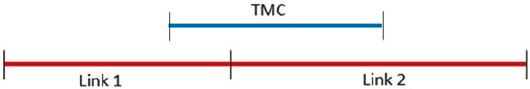
Some TMC segments may span across two or more defined volume link locations (if AADTs were provided by link segments instead of points), and vice versa (as shown in Figure 40). In order to obtain a single AADT measurement for TMCs that fall under this case, the AADT of the overlapped sensor locations must be weighted by the distance of the portion of the TMC that falls into the range of each link location.
Additional calculations are then made to break down the day of week ADTs into hourly profiles. The forementioned methodology for this follows closely the one defined by TTI in their 2021 Urban Mobility Report, Appendix A: Methodology (2021).
Event data from each source typically came with a latitude/longitude coordinate, road name, direction, start time, and an end time. Each event had to be map-matched with a specific TMC segment. At a high level, the methodology for incident and event map-matching (including for incidents derived from probe vehicles) is as follows:
- Search for the TMC segments closest to the latitude/longitude coordinates of the event.
- Of the returned results, identify TMC segments that have road names (or aliases) closely matching those associated with the event. For example, I-95.
- Of the remaining results, identify the closest segment that is in the same direction of travel as the incident report.
6.2.3.3 Use Case-Specific Fusion Algorithm
The bulk of the point-sensor and probe data fusion for this use case occurs in steps one and two of the fusion framework. After these basic fusion techniques are employed, the remaining algorithms are largely computational in nature and are simply using the results of the prior fusion to make some decision (Figure 41).
While spatial data fusion has already occurred in Step 2, there is additional spatial and temporal data checking that occurs later in this methodology, described in subsequent sections.

From the paper titled Identifying and Quantifying the Causes of Congestion—A New Tool for the Nation’s States and Counties to Better Understand the Contributing Factors to Traffic by Franz, et al. (2022), the following methodology is described and reprinted with minor edits and clarifications with permission of the author.
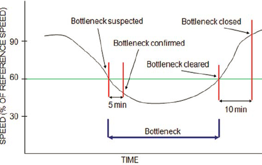
. . . the basis of the TDADS methodology begins with identifying when and where congestion occurs. Here congestion is defined as an observed speed that is 60% or less of the free-flow speed that is sustained for at least 5 minutes (Figure 42). Once these conditions were met, a bottleneck was declared to exist, and the quantification step was initiated. Here, delay was estimated each minute based on the speed drop and queue length associated with each bottleneck head location until the head location returned to at least 60% of the free-flow speed for 10 minutes (Lund, et al. 2017). The total delay for each bottleneck was computed by multiplying the delay by the impacted traffic volume and then aggregating the one-minute delays for the entire period that the bottleneck was active. Delay was estimated as both vehicle hours of delay and user delay costs. In this study, the traffic is assumed to be comprised of 90% passenger vehicles and 10% commercial vehicles. The value of time for passenger vehicles and commercial vehicles were adopted from the 2019 Urban Mobility Report (Schrank, et al. 2019).
The last step was to assign the total delay for each bottleneck to a causation category. As shown in Figure 33, this process began by looking at the temporal congestion pattern. If the delay pattern was similar to the historical pattern for the time of day and day of week of the target bottleneck, the bottleneck was categorized as a recurrent bottleneck. However, if the delay pattern was different, additional causes were considered. To identify recurrent patterns, the variations between the mean free flow travel time and the mean historical travel time were analyzed. In order to do this, you calculate the mean free flow travel time and the mean historical travel time across the TMC segments in the disruption queue for each minute of its duration. Once both values are calculated, the ratio of the free flow travel time to the historical travel time is taken. Similar to how a disruption is activated at 60% of the free flow speed, the ratio of the free flow travel time to the historical travel time is compared to a threshold of 0.60. Specifically, the recurrent nature of a disruption is classified based on the following conditions:
| (1) | |
| (2) |
Source: I-95 Corridor Coalition (2019)
It is worth noting that other causes can be paired with recurrent congestion to exacerbate delays. To consider such scenarios when the recurrent pattern is worse than normal, the following rules were applied:
| (3) | |
| (4) |
For all non-recurrent bottlenecks and recurrent bottlenecks plus additional cause(s), logic was developed to match the bottleneck location with a potential cause. The logic for each causation category was based on spatial and temporal boundaries as described below.
Incidents
The event data source is used to identify incident events to be matched to a disruption based on a mapping of event types to the incident category. The following spatial-temporal conditions are used to match the incidents (crashes), and events (disabled vehicles, debris, etc.).
-
Spatial:
- Condition 1: An incident/event TMC segment must be within the TMC segments in the queue of the disruption.
-
Temporal:
- Condition 2: The incident event created timestamp must be between the disruption start timestamp minus 5 minutes and the disruption closed timestamp.
- Condition 3: The incident event closed timestamp must be between the disruption start timestamp minus 5 minutes and the disruption closed timestamp.
For an incident/event to be matched, spatial Condition 1 AND either temporal Condition 2 or Condition 3 must be met.
Weather
Weather identification integrates two data sources: a) Waze, CV, or ATMS events and b) NOAA radar that has been conflated to the roadway. The Waze, CV, or ATMS data source is used to identify weather events to be matched to a disruption based on a mapping of event types to the weather category. The NOAA data source is used to identify precipitation (snow, sleet, and rain) that occurs during the disruption.
A. The following spatial-temporal conditions are used to match the weather events.
-
Spatial:
- Condition 1: A weather event TMC segment must be within the TMC segments in the queue of the disruption.
-
Temporal:
- Condition 2: The weather event created timestamp must be between the disruption start timestamp minus 5 minutes and the disruption closed timestamp.
- Condition 3: The weather event closed timestamp must be between the disruption start timestamp minus 5 minutes and the disruption closed timestamp.
For a Waze, CV, or ATMS weather event to be matched, spatial Condition 1 AND either temporal Condition 2 or Condition 3 must be met.
B. The following spatial-temporal conditions are used to match NOAA radar precipitation.
-
Spatial:
- Condition 1: The precipitation reading TMC segment must be within one of the TMC segments in the queue of the disruption.
-
Temporal:
- Condition 2: The precipitation reading timestamp must be between the disruption start timestamp minus 5 minutes and the disruption closed timestamp.
For a precipitation reading to be matched, spatial Condition 1 and temporal Condition 2 must be met.
Work Zones
The Waze, WZDX, ATMS, and/or Lane closure permitting system agency data sources are used to identify work zone events to be matched to a disruption based on a mapping of agency event types to the Work Zones category. The following spatial-temporal conditions are used to match the work zone events.
-
Spatial:
- Condition 1: A work zone event TMC segment must be within the TMC segments in the queue of the disruption.
-
Temporal:
- Condition 2: The work zone event created timestamp must be between the disruption start timestamp minus 5 minutes and the disruption closed timestamp.
- Condition 3: The work zone event closed timestamp must be between the disruption start timestamp minus 5 minutes and the disruption closed timestamp.
- Condition 4: The disruption start timestamp must be between the work zone event created and the work zone event closed timestamp.
For work zone events to be matched, spatial Condition 1 AND either temporal Condition 2 or Condition 3 or Condition 4 must be met.
Holiday Travel
A Holiday Travel Calendar is used to identify holiday travel days to be matched to a disruption. The following temporal condition is used to match the holiday travel days.
-
Temporal:
- Condition 1: The disruption start timestamp must be the same day as the holiday travel day.
Signals
The Open Street Map (OSM) Traffic Signal data source is used to identify signal locations that are matched to a disruption. The following spatial condition is used to match the OSM signals.
-
Spatial:
- Condition 1: The signal intersection TMC segment must be within the first two TMC segments in the queue of the disruption (i.e., the head of the disruption).
Multiple Causes
These are bottlenecks in which two or more congestion categories are present during the disruption. The delay associated with the multiple causes category was found to be significant in the preliminary exploratory analysis results, and it was determined that it should be further decomposed. Based on a sensitivity analysis in which CATT Lab sampled four months of data (February, May, August, and October) across seven states (AZ, CO, MD, MI, OH, VA, and PA),
the four most common combinations of congestion categories were identified. As a result of this analysis, it was determined that Causes of Congestion Graphs tools capture the following multiple-cause categories:
- Signal & weather
- Incident & work zone
- Incident & weather
- Recurrent & incident
- Other multiple causes (captures all remaining combinations)
In a similar fashion, if the congestion was deemed non-recurrent, alternative causes were assessed including multiple causes as well as an unclassified category for instances when a cause could not be determined. Each bottleneck was assigned to a causation category, and the results were then aggregated by month and county. The counties were aggregated to build the state results, and the states were aggregated to build the national results.
6.2.3.4 Quality Control
Unlike many ML applications, this use case does not include a training component or feedback loop in real time. Instead, quality control on the results is performed in two ways (Figure 43). First, quality control is performed on the incoming data during Step #1 to ensure there are not any gaps in coverage. Even small gaps of volume coverage—especially on major interstates in high-volume locations—can have dramatic impacts on the user delay that is presented.
Second, spot checking of expected user delay on select road segments is conducted on the results to ensure that the numbers make sense given the capacity of the roadway and measured congestion during any given period of time. Short-duration queries during known events can help to ensure that the results are reasonable and as expected. There is also an analysis of different geographies to check for variability. Analysts also look for seasonal variation to ensure variables such as weather, holidays, construction, and other causes change as expected.
Engineers who use the results of these analyses also provide feedback to systems implementers that is used to refine the base algorithms annually to ensure that they are still within expected norms. The CATT Lab is also conducting additional user delay studies that are not yet published but will provide additional insights in the near future.
6.2.4 More Information on this Use Case
For more information on this use case, please contact the CATT Lab at the University of Maryland by visiting the RITIS website at https://www.ritis.org or TETC’s website describing the early research effort at https://tetcoalition.org/projects/transportation-disruption-and-disaster-statistics/.


