Census Data Field Guide for Transportation Applications (2025)
Chapter: 13 Scenario: Understanding the Crucial-to-Identify Gaps in Transit

CHAPTER 13
Scenario: Understanding the Crucial-to-Identify Gaps in Transit
13.1 Overview
This scenario illustrates the use of ACS data with General Transit Feed Specification (GTFS) data to understand demographic and economic gaps and access to opportunities. Use of ACS data with GTFS data can help in understanding the characteristics of transit riders, including low income and majority minority and the transit supply available to them to access opportunities. (To ensure that the demonstrated analyses in this scenario are realistic, the fictional region portrayed in the scenario is based on an actual county.)
13.2 Background
The Two Seasons transit agency has the necessary funding to redesign its bus network for the communities it serves. The agency plans to engage an outside firm to perform the network redesign, but as part of laying the groundwork for the redesign, the agency wants to understand how well the current bus network serves the communities with low income and zero cars households. As part of this effort, Irene Adler, the Two Seasons project manager for the bus network redesign, designated Mycroft Holmes, a junior analyst, to analyze the current network and identify gaps and shortfalls.
The Two Seasons transit agency serves Capital County, where state government and education are major economic drivers, and where the county is trying to attract high-paying manufacturing industries to benefit from close collaboration with the universities in the county. The population of Capital County is just under 300,000, with a median household income of $58,118; 7 percent of households have no vehicles.
The Two Seasons transit agency is a bus-only agency and serves the population of Capital County using a hub-and-spoke network composed of 14 routes with weekday and weekend service. The agency serves predominantly transit-dependent and student markets.
Irene provided Mycroft with the following information:
- GTFS of the Two Seasons transit network
- 2017–2021 ACS data
- Table B02001 from the ACS—Race (Universe: Total Population)
- Table B08201 from the ACS—Household Size by Vehicles Available (Universe: Households)
- Table B25119 from the ACS—Median Household Income in the Past 12 Months by Tenure (Universe: Occupied Housing Units)
13.3 Analysis
Two Seasons, being a small agency, has pivoted to using open source tools and relies on QGIS (qgis.org) to help with its spatial analysis needs. Mycroft Holmes is experienced using QGIS and is comfortable using it to perform this analysis. However, not being familiar with importing GTFS files into QGIS, Mycroft turned to his colleague, John Moriarty, who had exported GTFS files into QGIS previously. As a first step, John told Mycroft to download the QGIS plugin GTFS-GO and install it into QGIS.
An alternative to QGIS is ESRI ArcGIS with a case study example available at https://learn.arcgis.com/en/projects/assess-access-to-public-transit/.
13.3.1 Importing GTFS into QGIS
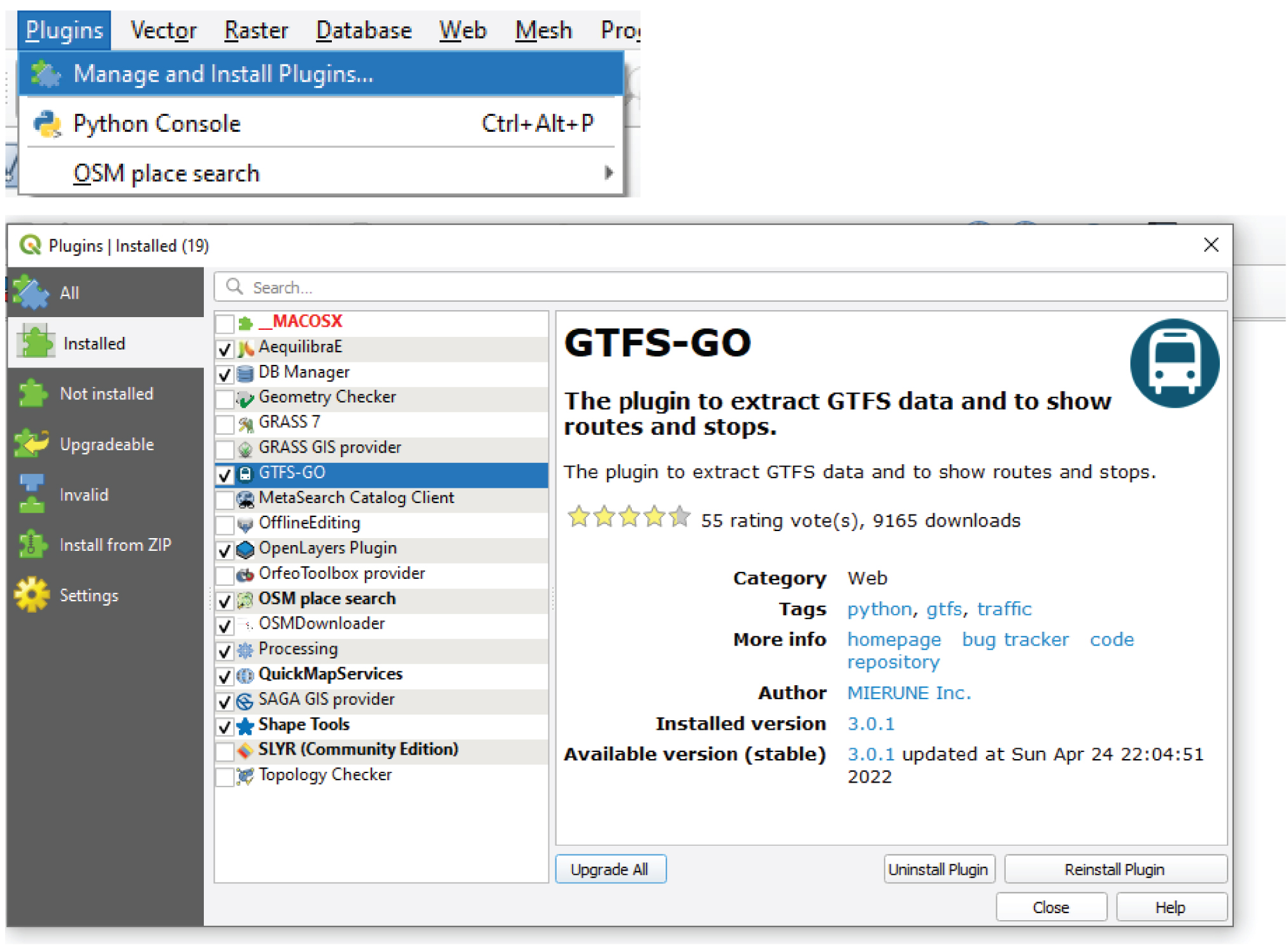
GTFS-GO is a plugin to extract GTFS data and to show routes and stops. It is available via the QGIS plugins add-in option (see Figure 13.1).
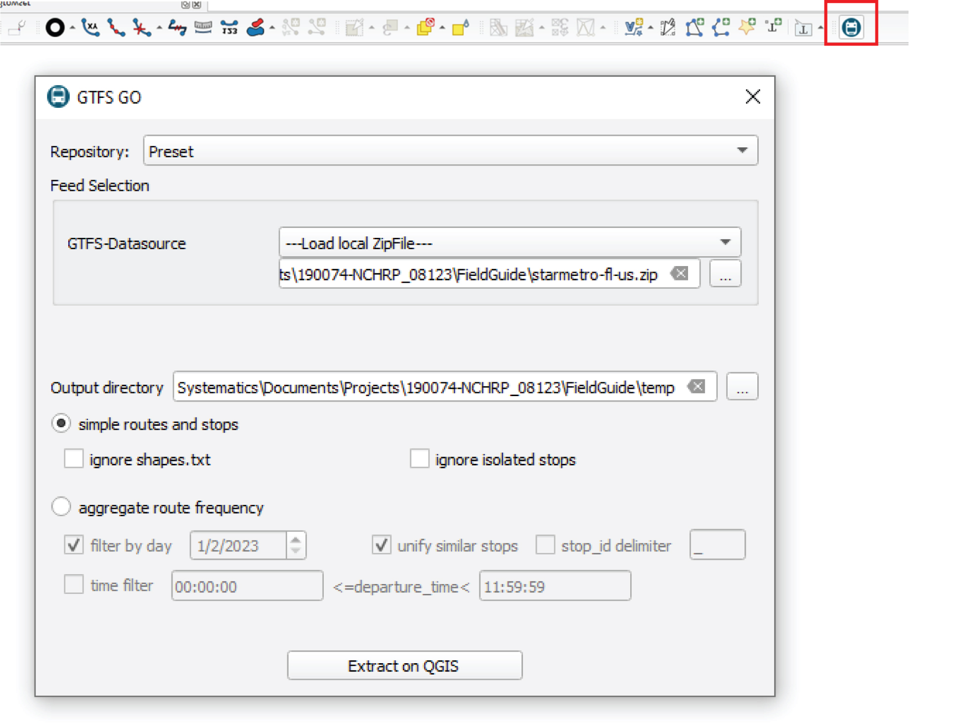
Once Mycroft installed the GTFS-GO plugin, he was able to import it into QGIS by loading the GTFS file provided by Irene and specifying the output folder where he wanted the resulting output file to reside. Figure 13.2 and Figure 13.3 show the GTFS import process and the resulting output, respectively.
Source: https://plugins.qgis.org/plugins/GTFS-GO-master/.
Long Description.
Two screenshots from the GTFS dash GO plugin are shown. The first screenshot has the Plugins menu open at the top with three listed options: Manage and Install Plugins, Python Console with shortcut Control plus Alt plus P, and OSM place search. The second screenshot has the Plugins window open with GTFS dash GO plugin selected. The plugin is used to extract GTFS data and to display routes and stops. The right section has plugin details such as category Web, tags like python, GTFS, and traffic, author MEIRUNE, Inc., version 3.0.1, and update date Sunday, April 24 22:04:52, 2022. The left panel lists plugin sections such as Installed, Not Installed, and Settings. Buttons at the bottom include Upgrade All, Uninstall Plugin, and Reinstall Plugin.
Long Description.
Two screenshots are shown related to the GTFS dash GO plugin used in a geographic information system. The first screenshot contains a toolbar with multiple tool icons; the GTFS dash GO icon is highlighted at the far right. The second screenshot contains the GTFS GO plugin window. The window has a repository option set to preset and a section titled Feed Selection where a local ZIP file is selected from a path ending in starmetro dash fl dash us dot zip. Below it, the output directory field is filled with a path ending in FieldGuide backslash temp. The route type is set to simple routes and stops, with options to ignore shapes dot t x t and ignore isolated stops. An alternative option called aggregate route frequency is present but not selected. Filter by day is checked with date 1 slash 2 slash 2023. Unify similar stops is also selected. Other filters like time filter and stop underscore i d delimiter are present but not active. At the bottom, a button labeled Extract on QGIS is available.

Long Description.
The digital map interface from QGIS shows a dense network of circular transit stop symbols each marked with a bus icon and lines representing transit routes; the Layers panel at the bottom left includes selected layers labeled stops and routes with route names such as Innovation IN, Nights B, Big Bend B, Forest E, Lake Oak L, Night S 2, Sunday Z, Cuco Loco DS, and Southwood VF; the Browser panel on the top left lists folder paths and spatial databases; the main view contains a network of transit stops connected by route lines forming a web-like pattern across the area; the toolbar at the top holds multiple tool icons and dropdown menus for project, edit, view, layer, settings, plugins, vector, raster, database, web, mesh, processing, and help.
Once the GTFS is successfully exported into QGIS as a geoJSON file (https://geojson.org/), the next step is to export the stops layer as a shapefile so that it can be merged successfully with the polygon (census tract) layer (see Figure 13.4). Alternatively, the geoJSON file can be joined directly to the census tract layer.
Resources for learning QGIS are available at https://www.qgis.org/en/site/forusers/trainingmaterial/index.html.
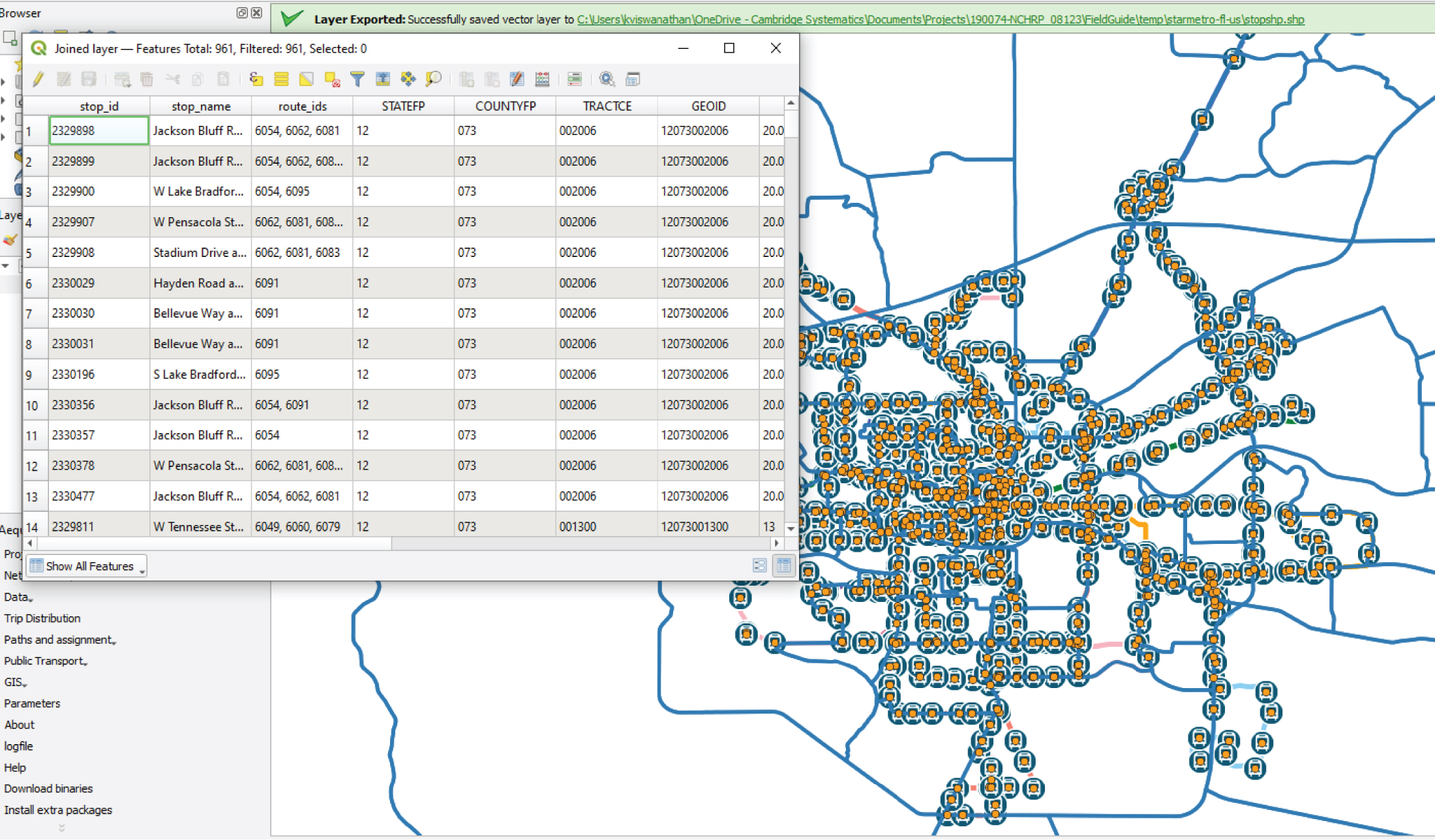
After importing the census tract layer into QGIS, Mycroft proceeded to join the attributes of the tract layer to the stops layer (see Figure 13.5). As part of this process, Mycroft wanted to make sure that each stop was contained within a census tract. The resulting shapefile along with its attributes is shown in Figure 13.6.
13.3.2 Layering Census Information to Transit Supply Attributes
As described in the previous section, Mycroft imported the attributes of the transit supply (stops and routes) into QGIS and tagged the stops with census tract GEOIDs. This gave Mycroft partial information on how well the transit system contributed to providing accessible opportunities for transit riders. Mycroft also learned about crucial-to-identify gaps in transit service that could be alleviated by the bus network redesign. Two Seasons provided transit service in 55 of the 79 census tracts in Capital County. Table 13.1 shows the distribution of stops by census tract in the county.
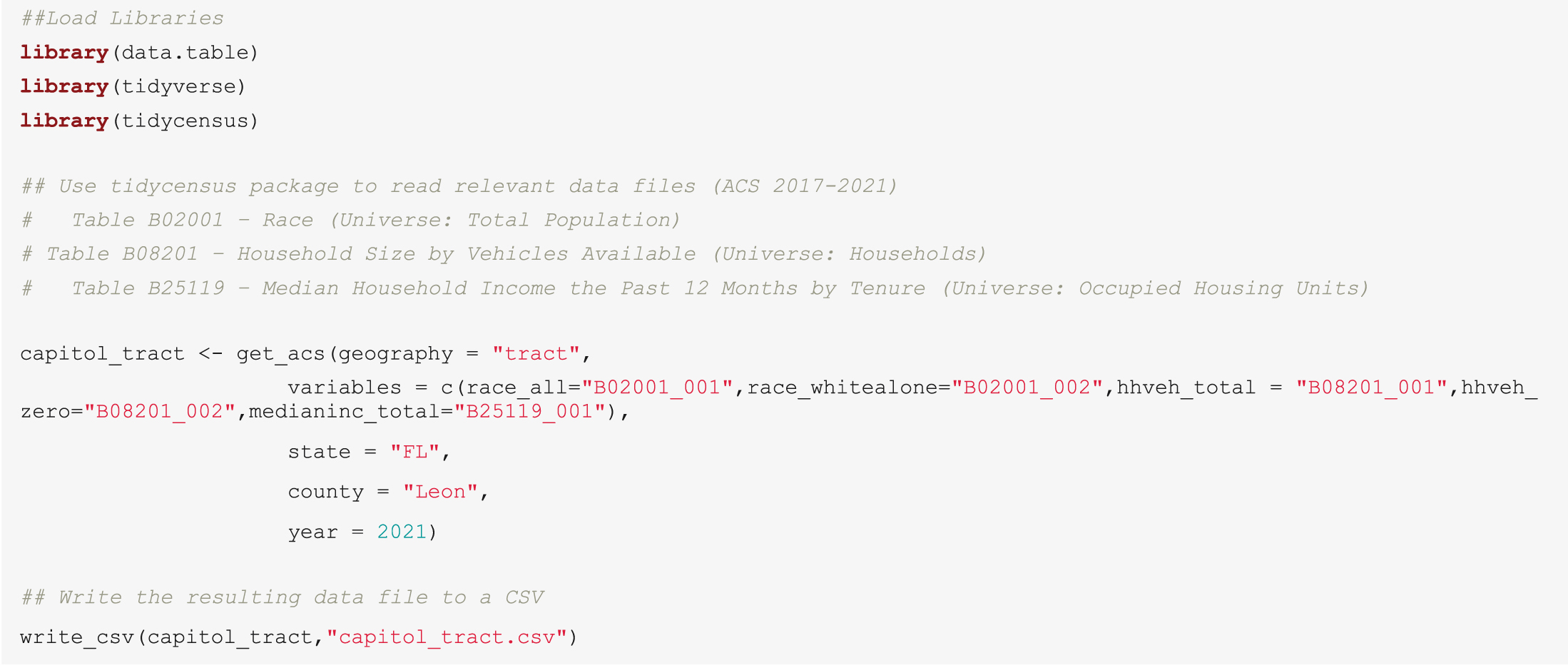
To identify if there was a discernible pattern in the number of available stops (which can serve as a proxy for accessibility) by census tract, Mycroft decided to map the distribution of stops by census tract based on communitiesʼ demographic and economic household characteristics. The first step that Mycroft took was to read the data via the Census Bureauʼs application programming interface (API) and the tidycensus R package (see Section 19.3 for additional details on the Census Bureauʼs API). Figure 13.7 shows the R code to get the data sample shown in Table 13.2 after transposing the data from long to wide format.

Long Description.
Two screenshots from QGIS are shown. In the first screenshot, the user right-clicks the stops layer under the starmetro dash fl dash us directory and selects Export followed by Save Features As from the menu. In the second screenshot, the Save Vector Layer As dialog box appears with Format set to ESRI Shapefile and File name field set to stop shp. The file is being saved in a directory path ending with starmetro dash fl dash us. Coordinate Reference System is set to EPSG 4326 WGS 84. The Save button is located at the bottom right of the dialog box. The process prepares the stops layer for export as a shapefile.

Long Description.
The interface has two parts. Two screenshots are shown.The top one displays the Vector menu opened in QGIS with the Data Management Tools submenu expanded and the Join Attributes by Location option selected. The bottom screenshot displays the Join Attributes by Location panel. The panel has Join to features in field set to stop s h p with coordinate reference system EPSG 4326. Features they intersect field has the option called are within selected. By comparing to field is set to leon underscore tracts with coordinate reference system E P S G 4269. Fields to add is empty. The Join type is set to create a separate feature for each matching feature. Buttons for Run, Close, and Help appear at the bottom. A description on the right explains that the algorithm creates a new vector layer by adding attributes from another layer based on spatial relationships.
Long Description.
The QGIS interface is shown with a shapefile layer of transit stops joined with tract attributes; the attribute table is open and lists fields such as stop underscore i d, stop underscore name, route underscore i ds, STATE FP, COUNTY FP, TRACT CE, and GEO ID; entries include stop names like Jackson Bluff Road and W Lake Bradford Road with associated route identifiers; the map view in the background contains symbols for stops over a network of lines representing tracts; a notification bar confirms the layer export with file path ending in starmetro dash fl dash us backslash stopshp dot shp; the attribute table displays a filtered total of 961 features joined with tract data.

Long Description.
The one-row table shows five categories: Minimum, 25th Percentile, Median, 75th Percentile, and Maximum. The Minimum is 1, The 25th Percentile is 9, the Median is 15, and 75th Percentile is 22, and the Maximum is 103.
Note: An electronic version of the R code used in the scenarios described in this report is available on the National Academies Press website (nap.nationalacademies.org) in the Resources section of the catalog page for NCHRP Research Report 1108: Census Data Field Guide for TransportationApplications.
Long Description.
##Load Libraries
library(data.table)
library(tidyverse)
library(tidycensus)
## Use tidycensus package to read relevant data files (ACS 2017-2021)
# Table B02001 – Race (Universe: Total Population)
# Table B08201 – Household Size by Vehicles Available (Universe: Households)
# Table B25119 – Median Household Income the Past 12 Months by Tenure (Universe: Occupied Housing Units)
capitol_tract <- get_a c s(geography = "tract",
variables = c(race_all="B02001_001",race_whitealone="B02001_002",h h veh_total = "B08201_001",h h veh_zero="B08201_002",medianinc_total="B25119_001"),
state = "F L",
county = "Leon",
year = 2021)
## Write the resulting data file to a CSV
write_c s v(capitol_tract,"capitol_tract.c s v")

Source: U.S. Census Bureau.
Long Description.
The table has 6 columns and 10 rows. The columns include GEO ID, household vehicle total, household vehicle zero, median income total, race all, and race white alone. Row details are as follows. Row 1. GEO ID 12073000200; household vehicle total 2,331; household vehicle zero 180; median income total 48,110; race all 4,193; race white alone 2,764. Row 2. GEO ID 120730000301; household vehicle total 690; household vehicle zero 35; median income total 69,583; race all 1,445; race white alone 1,077. Row 3. GEO ID 1207300302; household vehicle total 1,036; household vehicle zero 39; median income total 60,938; race all 2,189; race white alone 1,519. Row 4. GEO ID 12073000303; household vehicle total 1,845; household vehicle zero 142; median income total 38,678; race all 4,763; race white alone 1,371. Row 5. GEO ID 12073000400; household vehicle total 527; household vehicle zero 33; median income total 42,404; race all 2,565; race white alone 913. Row 6. GEO ID 12073000501; household vehicle total 126; household vehicle zero 11; median income total N A; race all 347; race white alone 347. Row 7. GEO ID 12073000502; household vehicle total 641; household vehicle zero 78; median income total 16,875; race all 2,270; race white alone 1,780. Row 8. GEO ID 12073000600; household vehicle total 1,355; household vehicle zero 424; median income total 22,832; race all 4,029; race white alone 1,414. Row 9. GEO ID 12073000700; household vehicle total 1,107; household vehicle zero 146; median income total 45,841; race all 2,041; race white alone 1,483. Row 10. GEO ID 1207300200; household vehicle total 2,331; household vehicle zero 180; median income total 48,110; race all 4,193; race white alone 2,764.
Table 13.2 shows the analysis of socioeconomic characteristics from the 10 study area census tracts. The variables that were studied were summarized at the tract level as follows:
- Total Number of households by vehicles available (hhveh_total)
- Total number of Households with zero vehicles (hhveh_zero)
- Median household income at the census tract level (medianinc_total)
- Total tract residents by all races (race_all)
- Total tract residents who identify as White (race_whitealone)
Given Mycroftʼs interest in understanding the current accessibility of the transit network and the communities it served, he tagged each census tract based on its demographic and economic characteristics. Table 13.3 shows the number of low-income tracts, the number of majority-minority tracts, and the number of tracts where the number of bus stops is fewer than the median of 15 stops.
Table 13.3 provides a regionwide summary of lack of access (via bus stops less than the median of 15 stops) along with information about tracts that can be considered low income and/or majority minority. However, the table does not provide this information in multiple dimensions and more importantly, does not indicate the location of the tracts that have fewer than 15 stops or those that can be considered low income and/or majority minority. Therefore, Mycroft decided to map the number of bus stops by low-income and majority-minority tracts.
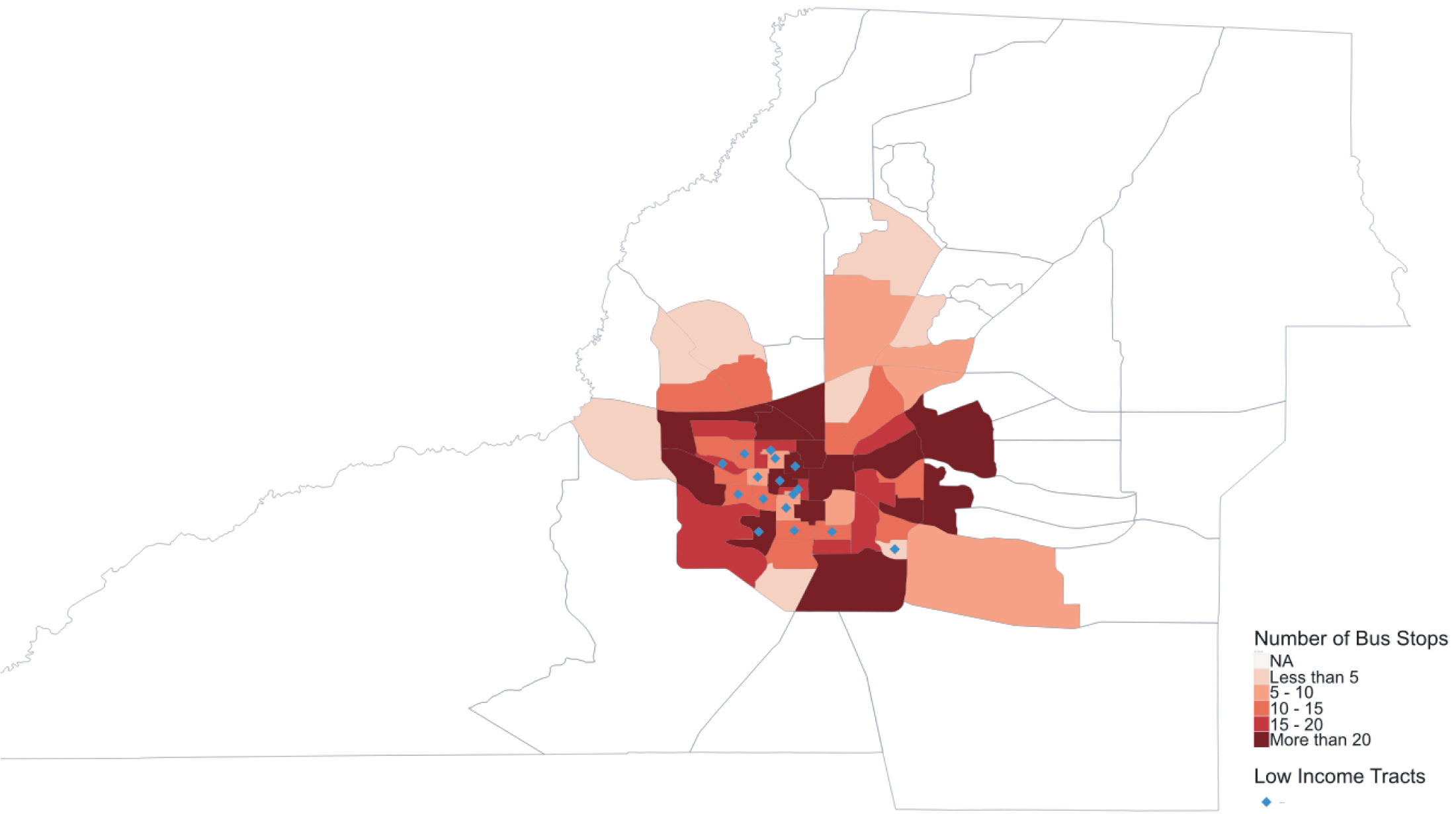
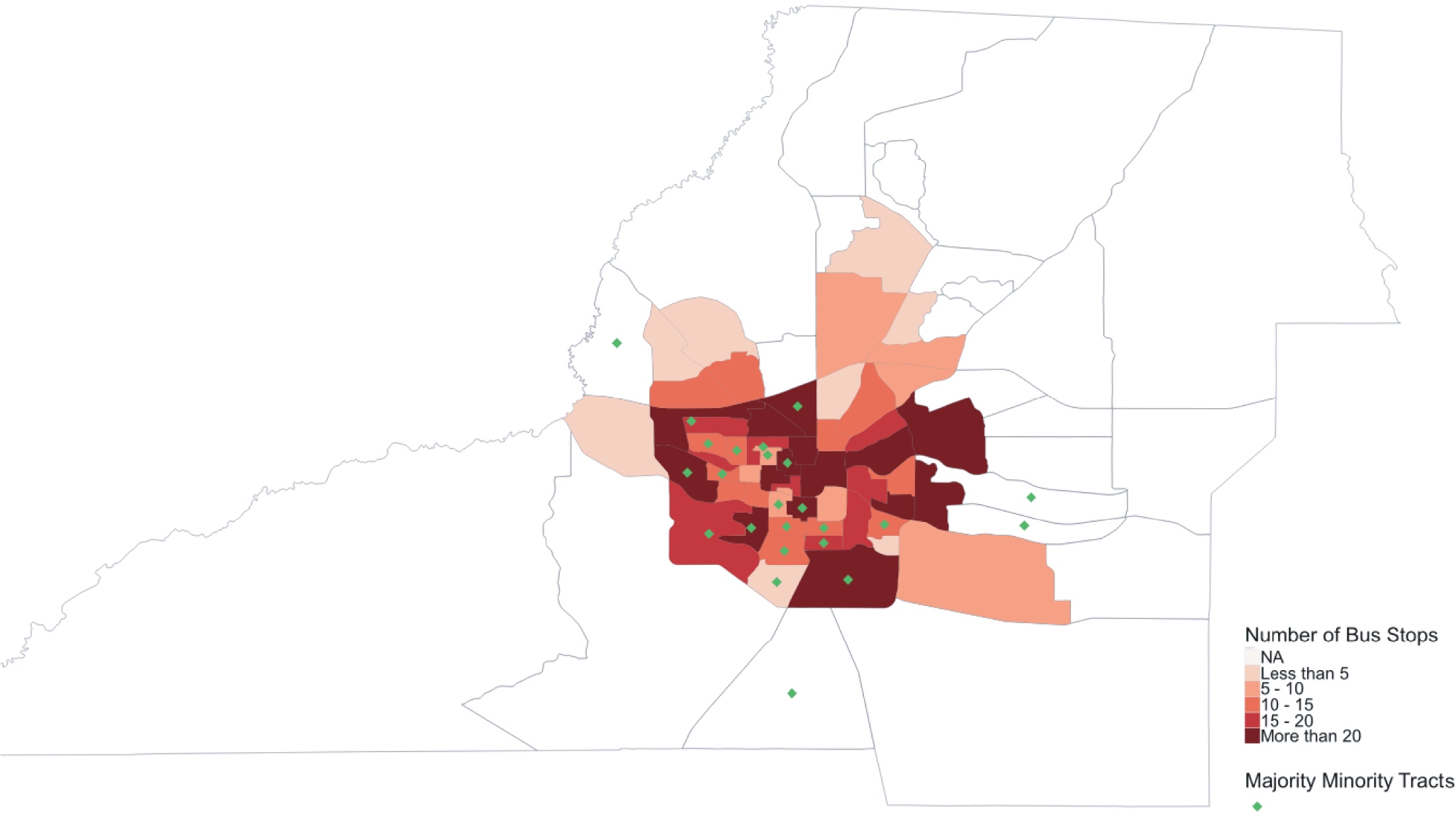
In the distribution of stops by census tract, Mycroft observed that most low-income tracts had the median number or more bus stops per tract (Figure 13.8), and he observed something similar with the majority-minority tracts. Some tracts had no bus service (Figure 13.9).
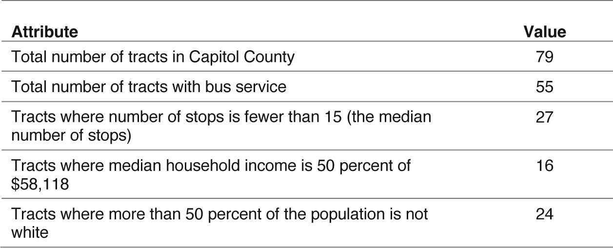
Source: U.S. Census Bureau and GTFS Data.
Long Description.
The table has two columns labeled Attribute and Value, listing five rows of statistics for Capitol County. The total number of tracts is 79, total number of tracts with bus service is 55, tracts where number of stops is fewer than 15 is 27, tracts where median household income is 50 percent of 58,118 is 16, and tracts where more than 50 percent of the population is not white is 24.
Long Description.
The map displays census tracts with shaded areas representing the number of bus stops categorized as NA, less than 5, 5 to 10, 10 to 15, 15 to 20, and more than 20; each tract is outlined and filled according to its bus stop count; diamond-shaped symbols are placed in several tracts to mark low income areas; tracts with higher numbers of bus stops appear concentrated near the center where most of the diamond symbols are located; the legend at the lower right explains the bus stop ranges and the symbol for low income tracts.
Long Description.
The map displays census tracts shaded by number of bus stops with categories labeled NA, less than 5, 5 to 10, 10 to 15, 15 to 20, and more than 20; each tract is outlined and filled according to the bus stop count; diamond symbols represent majority minority tracts and are placed across several tracts, mainly in central and southern areas; the legend in the bottom right corner defines the color ranges for bus stop numbers and the symbol used for majority minority tracts.


