can theoretically upload a wide range of telematic attributes, including braking/acceleration, occupancy, signal use, windshield wiper use, speed, and heading (i.e., direction of travel). Many of these features can directly serve safety research and very likely have never been made available at scale before. CVD data is almost always of higher quality because vehicle-based sensors are much more robust to disturbances that may confuse smartphones. CVD can identify the start and stop times of trips from the vehicleʼs ignition status, eliminating the need to infer the home and/or work location of the owners. These better preserve usersʼ privacy by reducing the collection of continuous location data. However, two issues with CVD include its bias towards newer vehicle models, which can create economic disparity, and its lack of coverage on VRU activities. On the other hand, CDR data is more suitable for tracking VRU activities because pedestrians and cyclists generally have a cell phone on their person.

Images from Mobile Sources

Images from mobile sources include satellite and aerial images as well as data collected by ground/street-level cameras.

Satellite images project objects onto a two-dimensional plane and offer a birdʼs-eye view of the Earthʼs surface. Satellite camera parameters are known, enabling direct distance measurements between points within the images. These capabilities make them particularly useful for understanding geometries. Satellite images can be collected by both commercial and public sources.

Aerial images are taken at much lower altitudes than satellite images. Raw aerial images inherently contain distortion caused by sensor orientation, systematic sensor and platform-related geometry errors, terrain relief, and curvature of the earth. Such distortions cause feature displacement and scaling errors, which can result in inaccurate direct measurement of distance, angles, areas, and positions, making raw images unsuitable for feature extraction and mapping purposes. Orthorectification removes these distortions and creates accurately georeferenced images with a uniform scale and consistent geometry. The orthoimagery tile system also makes it possible to convert between positional coordinates of tiles in x/y/z (where z represents the zoom level) and geographical coordinates.

Street-level images can be captured by dashcam or dedicated survey equipment. The latter group often includes street view images (SVIs) and panoramas, which are 360-degree surrounding images generated from multiple original images captured by a set of cameras and stitched together in sequences. Street-level images are widely used to understand urban scenes, particularly in infrastructure safety evaluation, because objects captured in these images reflect what drivers see while driving.

LiDAR

LiDAR scans allow distance to be directly calculated between any pair of points by producing point clouds in spherical coordinates (in the 3D space).

There are two kinds of ground-level mobile LiDAR datasets available for iRAP coding purposes. The first group of LiDAR datasets are vehicle-centered, where data are stored per timestamp/scene, similar to SVI/dashcam images. These LiDAR datasets are built to help train lighter and more accurate perception models that can be deployed on autonomous vehicles (AVs) to detect objects and understand driving environments. The second group of LiDAR datasets is infrastructure-centered, where data are stored per segment. This means moving objects are generally absent in the LiDAR point clouds unless they travel at identical or similar speeds with the survey vehicles. LiDAR sensors are also installed on roadway infrastructure to monitor critical

intersections/segments on the roadway network. They detect road users, i.e., vehicles, pedestrians, and bicyclists. Point clouds are collected by LiDAR in real time. They are usually processed by specialized software to generate categories, shapes, location, and speed information of the moving objects that are detected. LiDAR often works with video cameras to create reliable outputs. Local agencies are typically the point of contact to obtain LiDAR data.

Advanced Analysis Methods

With the rapid development of intelligent transportation systems (ITS), big data in the field of traffic are continuously collected from multiple sources over vast geographic scales. These big datasets are leveraged to conduct various research efforts in the field of traffic safety and provide new insights on safety analysis. With the capability of handling extremely large amounts of data, AI and ML approaches have the potential to provide a very high level of prediction accuracy for transportation safety analysis. Due to the nonlinear structures of AI/ML algorithms trained on relatively large datasets, AI and ML approaches have several apparent advantages, as shown in Figure 1. Since even very complex AI and ML algorithms can be implemented in real time with a minimal level of effort, these methods can greatly facilitate the identification of long-term traffic trends and short-term traffic patterns. Even with large amounts of data, especially high-dimensional data, AI and ML algorithms still have the capability to extract useful features and generate accurate prediction or classification results to support the safety-related decision-making of agencies. When an AI/ML model is well-designed and properly trained with enough data, the AI algorithm can be executed automatically without human intervention. Thus, AI-based analysis functions can be properly modularized to advance the implementation of safety analysis tools and platforms. Novel AI algorithms are even capable of transferring the learned knowledge from existing environments to new scenarios and can further help agencies take predictive actions to avoid possible crashes.

Mannering et al. (2020) and Lian et al. (2020) categorized AI and ML algorithms. These include instance-based algorithms, decision tree algorithms, Bayesian networks, dimensionality reduction

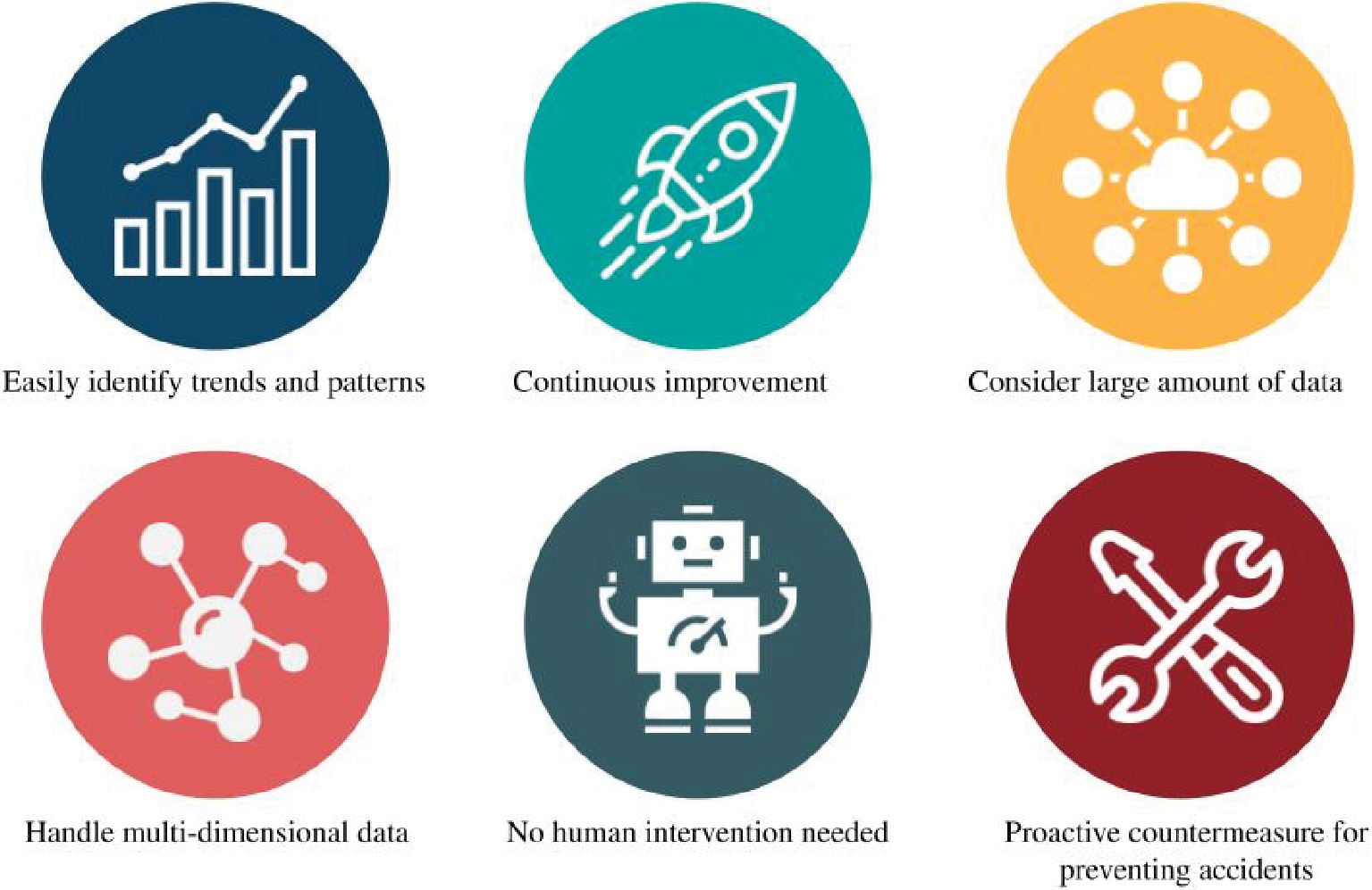
Long Description.

Each advantage of AI and ML is accompanied by text and illustration. The advantages of AI and ML approaches are listed as follows: 1, Easily identify trends and patterns. The illustration shows a set of bars with an increasing trend. 2, Continuous improvement. The illustration of a rocket is shown. 3, Consider large amount of data. The illustration shows a cloud with multiple branches. 4, Handle multi-dimensional data. The illustration shows a ball and stick model-like structure with multiple points. 5, No human intervention needed. The illustration of a robot is shown. 6, Proactive countermeasure for preventing accidents. The illustration shows a wrench and a screwdriver.

algorithms, and deep-learning-based algorithms, as shown in Table 2. There are also several existing systems for traffic safety analysis, such as “an artificial intelligence platform for network-wide congestion detection and prediction using multi-source data” (Wang et al. 2019). These AI-empowered, data-driven transportation platforms are capable of safety modeling, hot spot identification, incident-induced delay estimation, and traffic forecasting. Specifically, the safety performance module includes functions that can obtain traffic incident frequency, apply predictive models to estimate the safety performance of road segments, and visualize and compare observed incident counts and different predictive models.

Steps to Prepare Data for ML Analysis

When designing an ML system, seven key steps need to be considered. Most agency users apply the models but do not fine-tune/retrain their models, thus, they do not need to fully understand the technical steps. However, it is still advised to maintain a basic understanding of these technical steps while giving the planning steps full consideration to understand the modelʼs limitations and the gap between them and the agencyʼs desired use case. This may not be clear from the researcher/model developerʼs perspective, but the agency should pay attention to it. Traffic sign detection and recognition is one example of the seven steps, which is discussed here, with each data source described in greater detail.

Seven Key Steps to Designing an ML System

1. Clarify requirements. Define the problem, scope, data availability, and expected use case.
2. Frame the problem as an ML task. Specify system input and output and determine if research and development (R&D) is needed.
3. Data preparation. Acquire, store, and prepare data for training and testing.
4. Feature engineering. Apply techniques to enhance data for model training.

5. Model development. Design and develop the ML model architecture.
6. Model training. Train the model using appropriate software and hardware.
7. Evaluation. Set benchmarks, choose evaluation metrics, and analyze performance.

Example Application: Traffic Sign Detection and Recognition

• Clarify requirements: Agency X wants to update its traffic sign inventory to prepare for a safety project that will help them understand if there is a relationship between the density of speed limit signs and speeding behaviors.
  • Problem scoping: Collect locations (latitude/longitude coordinates) of all speed limit signs and the signsʼ speed limit readings on agency Xʼs roads, which could include streets, arterials, highways, and/or freeways of all functional classes.
  • Data availability and gaps: Image data are available for state highways and freeways. Similar to Washington State Department of Transportationʼs (WSDOT) SRweb application (state route web tool) and ODOTʼs Digital Video Log, these image data are recorded in sunny weather, at every 0.01- or 0.005-mile increment in both directions, and are of good visual quality. The agency has no data for local roads/streets/arterials and understands this is a gap they are currently facing.
  • Expected use case: The agency does not have specific requirements regarding the deployment of the model (e.g., on survey vehicles). Nor does it expect the model to run and produce the inventory in real time (e.g., autonomous driving signs are expected to be recognized in real time).
  • Decide if ML is needed: The agency wants to use ML models because they have been proven reliable and close to human performance in similar transportation tasks. They are less costly than human annotation in the long run. In this project, though, the agency decided to ask an engineer to double-check the results produced by ML models.
  • Existing models and products: The agency has performed a preliminary search into existing open-source ML models. They found that existing models are trained on several major open-source datasets, but most of them are not collected in the United States. The agency wants to follow the definition from the Manual on Uniform Traffic Control Devices (MUTCD) so that the model can be applied for other sign recognition and inventory collection purposes beyond this project.
• Frame the problem as an ML task.
  • Specify system input and output: The model is expected to detect traffic signs in the images fed to it and recognize their corresponding classes following MUTCD. In addition, their locations will be recorded in latitude/longitude coordinate formats.
  • R&D expectations at the agency: In previous steps, the agency has identified gaps between the expected use case (e.g., follow MUTCD categories) and existing open-source models. There might also be a lack of efforts specifically targeting the conditions or data of the state in which the agency operates, although this is of lesser importance. The agency expects R&D activities and outsources them to an academic research partner who will train and produce a model.
• Data preparation.
  • Data acquisition and storage: Data tends to be more accurate from a larger sample size and more recent sources. However, considering specific project needs, there are three ways to acquire image data. Ranking by quality and relevance, these include self-collected, acquired through application programming interfaces (APIs) of commercial mapping services, and via open-source datasets. Self-collected data are ranked first because the agency may already have a data collection campaign for other purposes with similar data that can be applied to the current project. Moreover, in this scenario, the agency has better control over the surveying activity and has access to the equipment configurations. Sometimes, downstream functions need these parameters of configuration to perform more

• calculations. The second way to acquire data is from APIs of commercial mapping services. This data source can provide geographical coverage (e.g., Google Maps, Mapillary, OpenStreetCam, Apple Look Around, and Bing Streetside), but quality could vary. The infrastructure assessment would typically require recent inventory data, but available SVIs may have been collected several years ago, and there is no control over the quality of such data. Therefore, data from third-party APIs can be used at large scale to identify trends and general patterns; however, caution needs to be taken when these data are used for microscopic analysis, such as in this project. Finally, public datasets are common sources used to train ML models. If the agency wants to conduct R&D (i.e., train ML models themselves), then these datasets are necessary. On the other hand, if the agency does not train a new model, then its efforts should focus on the first two sources. This is because public datasets used to train ML models typically have limited local coverage. In this narrative, because agency X wants to perform traffic sign inventory collection for its roads, it is advised to focus on self-collected or API-acquired data. Image data typically do not require special storage software or protocols. Saving them on disks and in properly named directories is appropriate.

• • Prepare for training: As will be discussed in the next major step, image data require certain feature engineering and augmentation. This preprocessing is typically performed during training (i.e., the code scripts will perform preprocessing in memory and will not save intermediate results). As the agency is delegating R&D to an academic partner, the agency itself need not worry about preprocessing for training. However, as data are fed to model training, they need to be properly labeled and annotated. The academic partner may reach back out to consult on data labeling. In this narrative, the traffic signs in the training data need to be localized in the images and properly categorized. Labeling the locations may require special tools so that the bounding boxes can be drawn correctly and tightly, while labeling corresponding classes for each captured traffic sign may be simpler. In summary, there is not usually much preprocessing work required for training data at the agency.
  • Prepare for testing: Similar to training of the model, model testing requires labeled data. In this narrative, the agency spoke with the academic partner and decided that the academic partner would label test road segments designated by the agency (much like what they would do for training data).

• Feature engineering.
  • Feature engineering is a required step during model R&D. As modern deep learning models can contain millions to billions of parameters, more training data of higher quality is always wanted. To create a meaningfully large training dataset, images are augmented (e.g., cropped, rotated, flipped, and/or mixed). Other feature engineering practices for ML applications can include necessary image resizing, color correction, and more. This step is typically programmed as functions in the code scripts.
• Model development.
  • The researchers need to investigate appropriate structures. Following previous discussions, the model is expected to detect traffic signs and identify their classes. Recording locations of speed limit signs can then be achieved through additional functions.
• Model training.
  • Software: Training an ML model involves updating its parameters in the order of forward propagation and backpropagation. During the forward propagation, the model is given the input image and estimates the value/label. Compared with the ground truth label, a loss is calculated. This loss signal is then propagated back to update all or selected parameters in the model. To reasonably train an ML model, researchers will need to specify appropriate loss functions and other hyperparameters.
  • Hardware: Choosing the right hardware is also critical to training modern ML models because they are becoming increasingly large. Graphics processing units (GPUs) are essential for these computation-heavy workloads. The size of the ML model should fit in

• • appropriate GPU memory. Two options are usually considered for computing hardware: Purchasing physical GPUs and training models locally or adopting cloud computing services and training models on the virtual GPUs. The trade-off is either fixed/overhead costs of physical GPUs or variable costs of cloud computing.
• Evaluation.
  • Set up the benchmark: One common strategy for evaluation involves asking the model to train and test on two different datasets. The agency may deliberately withhold a selection of particularly challenging scenarios—such as intersections with atypical layouts or images captured under extreme lighting or weather—from the training dataset. These challenging cases are then used exclusively for testing to evaluate the modelʼs ability to generalize to unseen data.
  • Choose metrics: For this particular task, the success of the model(s) will be evaluated based on the rate of detection (e.g., how many signs in the images are detected or missed) and the correctness of recognition (e.g., how many signs are categorized correctly). Setting up the evaluation metric can also help researchers design or choose their loss functions.
  • Examine negative examples: After the model is developed and tested on designated data, it is important to investigate negative examples in addition to producing the numeric metrics. While numeric metrics are sufficient for overall model performance, they may not be informative enough to reveal where the model fails. For example, a model that consistently fails on images collected with tree backgrounds and on cloudy days is worse than a model that fails without a specific pattern. The former may have huge implications for agencies that encounter that situation often.

After introducing the general concept of how to plan and scope an ML system, the next few paragraphs will discuss several major data sources, including both classical and emerging ones, and how they can contribute to iRAP roadway safety assessment and common processing procedures.

Examples of Data Sources to Be Used in iRAP Roadway Safety Assessment

Loop detector data are an accessible data source commonly used for traffic operations analysis. They contribute to the operating speeds in iRAP assessment framework. In addition, they can produce classified vehicle volumes that are critical for adjusting traffic flow parameters, given their distinct operating characteristics compared to passenger cars. This includes slower acceleration, inferior braking, and larger turning radii. Loop detector data can be accessed at data portals maintained by state departments of transportation (DOTs). At the WSDOT, for example, vehicles are classified into four bins or categories based on length, and the counts per bin are recorded at dual-loop detectors. These counts are the dependent variables, and the predictive features are provided by single-loop detectors. A general procedure is suggested for data quality control before feature extraction. This quality control step should check for and correct the following errors: segmentation, volume over range, stuck, not reporting, volume/occupancy ratio over threshold, and late-night zero volume/occupancy ratio. After the data quality is properly controlled, the dataset for classified vehicle volume estimation can be set up. Because traffic flow composition can vary by site, lane, and bin, it is advised to set the dependent variable as the number of observed counts for the selected bin and lane per time interval, and to set speed, volume, and occupancy from the corresponding single-loop detector in the last time window. The time granularity and length of the prediction window depend on the userʼs specific application and data availability. In this study, each time step is 20 seconds, and features are collected over the preceding 5 minutes (i.e., 15 consecutive 20-second intervals). Concretely, to predict the classified-vehicle volume for the current 20-second interval at time X, speed, total volume, and occupancy are aggregated and recorded by the corresponding single-loop detector during

the 15 intervals spanning X – 20 seconds to X – 300 seconds (or X – 1 to X – 15 time steps). This rolling 5-minute feature window captures recent traffic dynamics while remaining short enough for near real-time prediction.

Street-level images can contribute to the automated coding of multiple iRAP variables. Given that videos recorded by onboard survey cameras are the default data source for manual coding, it is important that street-level images contain most of the information needed for corresponding variables. The challenge is to acquire the right data and design effective ML methods that can extract the desired information. There are three typical sources of street-level images. First, highway systems could have been covered by existing data collection efforts at the agencies (e.g., WSDOTʼs SRweb application and ODOTʼs Digital Video Log). Images made available by these applications are extracted from recorded videos and are made available every 0.01 mile or even less. This spatial granularity is enough not only for iRAP purposes but also for specific tasks such as the one the research team performed in a pilot study. The greatest advantage of this source is the consistent quality of the collected data, while the challenge is the inability for batch download, typically limited by the agenciesʼ systems. The second way to acquire street-level images is via map service providers and APIs, e.g., Google Maps, Mapillary, OpenStreetCam, Apple Look Around, and Bing Streetsider. Images can be efficiently downloaded by a computer program, which passes several parameters to the API. For example, the research team followed the instructions given at Google Maps API Developer Guide and used a Python script to download an SVI on I-5 in Seattle, WA. While this method provides universal access to street view data, the user will have limited control over the time, exact location, and weather conditions of the returned image. This could be a problem if the user wants to analyze 2024 data, but the most recent data were collected in 2021, and the surroundings changed in that time due to a construction project. This method will also incur costs based on the number of images downloaded.

The third source is public datasets. As autonomous driving is pursued, companies and research institutions have collected open-source data covering different locations and scenarios. For example, CityScapeʼs dataset collected urban street scenes in 50 German cities; nuScenesʼs dataset collected LiDAR and images from Boston and Singapore. These data tend to focus more on road users, e.g., pedestrians and vehicles, rather than on infrastructure elements. This means the roadway infrastructure item captured may not be appropriately labeled/annotated. Secondly, these data may never be local to an interested user because the coverage of the data collection efforts is limited. As modern ML pipelines include feature engineering functions, there are no general data preprocessing procedures to follow. However, a key guiding principle is that the input data should be aligned with the specific requirements and characteristics of the intended use case. In other words, models trained in one setting, e.g., location and daytime/nighttime, may not transfer well to another. Task-specific quality controls are needed. To summarize, street-level images provide visual information of the roadway closest to the driving experience and can typically be acquired from three sources. It is advised that public autonomous driving datasets be used as training data because they can be accessed in large quantities, typically for free, and are well-annotated. Agency data or data acquired from map service providers can then be used in specific tasks, forming a smaller case-specific dataset for fine-tuning and testing models.

Geospatial mobility data contributes to iRAP assessments in multiple ways. Cell phone location data can be mapped to critical intersections and/or road segments to infer volumes, activities, and behaviors of active users. CVD are widely used for estimating roadway operating speeds; the extracted braking behavior (e.g., brake rate and hard brakes) and queueing at intersections could also be used as indicators of operational performance and signal timing plans, respectively. Several iRAP variables, such as the quality of the intersection, can adopt such extracted behavioral features as indicators. Large-scale GPS-based mobility data primarily come from commercial vendors. While regional organizations may collect household travel survey responses that include respondentsʼ trips, the quality of these data can be limited because they are designed to

serve planning goals rather than safety improvement goals. For example, the temporal granularity can be several minutes and even hours, while spatial granularity can be coarsened when exact latitude and longitude recordings are obscured for privacy concerns. Geographic boundaries (e.g., city limits or census tracts) and time windows are specified to estimate the number of observations, which are the basis of data purchase prices. CVD are almost always superior to cell phone data in terms of quality. Modern connected vehicle datasets can achieve 3 seconds temporal granularity, 10 ft spatial accuracy, and a 5% to 10% penetration rate (in most cases and after quality control). Due to this difference in quality, the preprocessing steps for cell phone location data vs. connected vehicle data are very different. Cell phone location data typically need data cleaning on three dimensions: consistency, accuracy, and completeness. According to Hu et al. (2021), the consistency dimension defines contextual semantic rules in order to keep only valid and deduplicated records. One record per second is kept at most. The accuracy dimension typically checks for noisy and extremely inaccurate observations based on geospatial knowledge of the application. Then, depending on the specific application, different steps are taken to finalize the preprocessing, e.g., home and work locations are inferred from multiday data for planning studies, and time intervals are checked to remove jump points for valid walking traces that cross streets. Smoothing is a universal quality control step for connected vehicle data, where raw GNSS coordinates are processed with a median filter, a Gaussian filter, or local regression. The vendor can complete this smoothing step before shipping the data products. Most applications then require the smoothed trajectories to be matched to maps. This is because features will be extracted and aggregated per road segment and/or intersection. Also, distances to objects need to be measured per record, for example, for a time-space diagram at an intersection. One scalable map-matching solution is the Open-Source Routing Machine (OSRM), which can match vehicle trajectories to the OpenStreetMap (OSM) road network.

LiDAR point cloud data can be used for iRAP assessment by extracting features of roadway infrastructure, including but not limited to the number of lanes, the width of each lane, median type and width, shoulder characteristics, overhead distance for bridges, intersection type, and roadside objects. LiDAR point cloud data need to be properly processed to extract these characteristics, taking into account the specific attributes of these points. Typically, LiDAR point cloud data are collected using sensors mounted on moving vehicles, which use lasers to measure distances. These lasers emit light pulses towards the ground and measure the time it takes for the light to bounce back. These mobile platforms capture detailed three-dimensional attributes of roadways and their surroundings. The high-resolution data generated provides a comprehensive view of the topography and visible surface features, including road infrastructure. The features of point clouds could vary based on the specific sensors used during data collection. For example, some LiDAR datasets include the color [i.e., red, green, and blue (RGB) values] of each pixel, while others do not. One major challenge with LiDAR data compared to other data sources, such as SVIs, is the high cost of collection, which limits access to large datasets for model training and extensive research. First, the raw LiDAR data needs to be preprocessed to remove noise and irrelevant information. Techniques such as segmentation and classification algorithms are employed to isolate the points that specifically represent the road surface and its features. Within the road surface, elements such as lanes and markings are identified based on reflectivity and geometric patterns. This segmentation is crucial as it helps isolate specific road features necessary for detailed analysis. By analyzing the density and arrangement of the point cloud over road surfaces, algorithms can detect variations that correspond to lane boundaries and markings. These algorithms can distinguish painted lines on the road, which often reflect lasers differently than asphalt. These data can then be used to calculate the number of lanes, the width of each lane, and the characteristics of shoulders and medians. Advanced computational techniques, such as ML models, can be applied to enhance the accuracy of feature detection and automate the extraction process. These models should be trained on vast amounts of LiDAR data to accurately

recognize and predict roadway features. In summary, LiDAR point cloud data has significant potential to assist in automating road safety enhancement practices. Models can be developed to extract detailed data regarding road characteristics with a high level of accuracy.

Introduction to Example AI/ML Methods and Applications

This user guide also demonstrates the methods and application of AI/ML algorithms and big data analysis with research examples. The research team applied these methodologies to eight different research topics.

The research team conducted two in-depth pilot studies, described in Chapter 4, each serving as a proof of concept for methods introduced during the research.

• Capturing new data with ML, ODOT. Applied the AI/ML models developed by the research team to detect and locate streetlight luminaires for the ODOT highway network in their Region 1, using ODOTʼs inventory and Mapillary imagery as the data source. This would help the streetlight luminaire inventory improve crash risk analysis in Oregon.
• Analyzing big data, City of Bellevue, WA. Examined how intersection video analytics can be used for a more in-depth analysis of road user behaviors, including turning vehicle speeds and trajectories. If these behaviors correlate to the geometries of these intersections, then designs can be modified to reduce vehicle speeds and change the angle of approach. This can improve safety for pedestrians and bicyclists in the intersectionʼs crosswalks.

The team conducted six follow-up research studies, described in Chapter 5, each of which builds upon the tools developed and methodologies studied as part of this research effort.

• Classified vehicle volume from loop detector data. Demonstrated how AI/ML can be used to model classified vehicle volume with single-loop detector data. Extending classification to the relatively high density of real-time traffic monitoring stations in urban areas could help traffic management systems better monitor freight traffic within metropolitan areas.
• Turning movement counts from CVD. Explored and validated principled pipelines applied to connected vehicle GPS data for TMC data at intersections.
• Lane markings and width from LiDAR data. Captured detailed topographical information, including the presence of road markings, curbs, barriers, and other vehicles, to gain a comprehensive view of lane boundaries, road width, and the orientation of the lanes in relation to the vehicle. Findings can help enhance the safety and reliability of autonomous driving technologies.
• Traffic sign detection and recognition from road log videos. Developed an automated tool for TSD and traffic sign recognition (TSR) using computer vision (CV) and deep learning techniques. An automated system would aid advanced driver-assistance systems (ADAS) and improve management and operational efficiencies.
• Pedestrian detection from mounted surveillance cameras. Processed surveillance camera videos of pedestrian crowds frame by frame via the scale-aware representation learning empowered sensing (SARLES) algorithm (Liu et al. 2024). This advanced tool can assist traffic agencies with sophisticated transportation management, safety issue monitoring, and traffic operations.
• Road surface condition from edge devices. Built AI/ML algorithms to identify complex patterns, improving the accuracy and efficiency of road surface condition detection. The research teamʼs AI/ML-based software also detects congestion, operating speeds, classified vehicle volume, and road user behaviors to support proactive crash prevention.