Implementation of A Guide to Computation and Use of System-Level Valuation of Transportation Assets (2026)
Chapter: Appendix B: Case Studies
B-1. Calculating Asset Value for Pavement Base and Surface in a Midwestern Agency
Summary
In this example, a state department of transportation in the Midwest, anonymized as the “Midwestern DOT,” calculated asset value for its pavements by separating the pavement into two components (the pavement base and the pavement surface) and calculating value for each component independently. This approach allowed the agency to develop a more nuanced asset valuation for pavement that accounts for the unique depreciation and lifecycles of both components.
Background
The Midwestern DOT’s primary driver for calculating and reporting asset value is to comply with the Federal Highway Administration’s (FHWA) requirement that State DOTs include a calculation of the value of National Highway System (NHS) pavement and bridge assets in their transportation asset management plans (TAMPs), and that they calculate the cost of maintaining asset value (23 CFR § 515.7(d)(4)).
For previous iterations of its TAMPs, the Midwestern DOT calculated pavement asset value using a replacement cost approach that did not account for age or condition data and therefore failed to reflect depreciation. The calculation also did not include a meaningful estimate of the cost to maintain asset value, since the cost to maintain replacement value remained $0. In addition, the approach did not delineate pavement components or recognize the different rates at which they degrade. To improve the usefulness and accuracy of its asset valuations as well as generate a cost to maintain current value, the Midwestern DOT developed an improved valuation approach that depreciated and valued the base and surface of the agency’s pavement separately.
Methodology
Data
The Midwestern DOT used a state performance measure based on pavement distress data to measure the condition of the pavement surface, and age based on the year constructed to measure the condition of the pavement base. Existing unit replacement costs were reused from asset valuation calculations to remain consistent with agency practices.
Pavement Layers
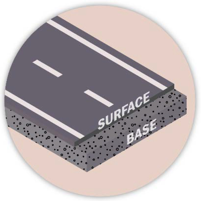
The pavement base and surface layers, shown in Figure B-1.1, were separated in this asset valuation process because they differ significantly in how they deteriorate and how they are managed. The base has a longer lifespan, is reconstructed infrequently, and is assessed using age, while the surface deteriorates faster, is replaced more frequently, and is evaluated based on distress data collected by the Midwestern DOT. These layers also have distinct costs and treatments, with the agency managing them separately in practice. By treating them as separate components, the valuation more accurately reflects their different roles in pavement performance.
Pavement Base Approach
The approach for valuing the pavement base layer assumed linear depreciation by year, where the end of life for a pavement base was defined as 60 years for Interstate pavements and 90 years for non-Interstate pavements. Pavement base age was defined by the year of initial construction. For a given pavement section, percent remaining value is calculated as the ratio of the current pavement base age to the end of life for that pavement.
Pavement Surface Approach
Valuation of the pavement surface used a condition-based methodology. The Midwestern DOT used existing deterioration models for the pavement surface to establish an effective asset life for each pavement family, as defined by the agency. The effective asset life was determined based on the time taken to deteriorate to the end-of-life threshold, at which point the asset was considered fully depreciated (valued at $0). The Midwestern DOT defined the pavement surface end of useful life as a condition rating of 4 for Interstate and a rating of 3.5 for non-Interstate pavement. The agency also calculated the current effective age of the pavement surface for each section and used that value to compute the percent remaining value for each pavement section (ratio of the current effective age to the effective asset life).
The Midwestern DOT used the approaches to calculate asset value for each layer and combined the results to get an overall asset value. In addition, the agency calculated a cost to maintain value and asset consumption ratio (ACR) for each approach. The valuations were performed in a spreadsheet tool where the agency could adjust parameters including the pavement base lifespan, the pavement surface condition end-of-life threshold, the rehabilitation cost per centerline mile, and the replacement cost per centerline mile. This tool allowed the Midwestern DOT to explore the impact of these parameters on the results.
Results
Table B-1.1 details the calculation of asset value for the Midwestern DOT’s pavements. The table shows replacement value, remaining asset value, ACR, and cost to maintain for the pavement surface, base, and total. The results are summarized by System (Interstate, Non-Interstate NHS, Non-NHS).
Table B-1.1 Asset Value Results
| System | Replacement Value by Method ($B) | Remaining Asset Value by Method ($B) | Cost to Maintain by Method ($M) | ACR by Method (%) | ||||||||
|---|---|---|---|---|---|---|---|---|---|---|---|---|
| Base | Surface | Total | Base | Surface | Total | Base | Surface | Total | Base | Surface | Total | |
| Interstate | 28.8 | 13.0 | 41.7 | 4.6 | 5.9 | 10.6 | 310 | 343 | 653 | 16 | 46 | 25 |
| Non-Interstate NHS | 35.5 | 8.0 | 43.5 | 6.4 | 5.0 | 11.4 | 196 | 320 | 515 | 18 | 62 | 26 |
| Non-NHS | 56.3 | 12.7 | 68.9 | 4.8 | 7.0 | 11.8 | 210 | 546 | 756 | 9 | 56 | 17 |
| Total | 120.6 | 33.5 | 154.1 | 15.9 | 17.9 | 33.8 | 715 | 1,209 | 1,924 | 13 | 53 | 22 |
Lessons Learned
Lessons learned from the Midwestern DOT’s exploration of an asset value approach for pavement base and surface include:
- Dividing an asset into components can yield improved asset valuation results when data are available, particularly when the components have very different useful lives.
- For example, while the value of the pavement base is nearly four times the value of the pavement surface, the cost to maintain value is lower for the pavement base than for the pavement surface. The lower cost to maintain value for the base compared to the pavement surface is to be expected given the pavement base has a useful effective life of 60 or 90 years, while the pavement surface has an effective useful life of 14-42 years.
- Calculating a separate remaining value for each component allows agencies like the Midwestern DOT to account for their unique characteristics, such as:
- Different deterioration rates and behaviors of the components.
- Different data sources available for components. For example, condition data was only available for the pavement surface, while the base layer was limited to the year of construction.
- The wide range of treatment and replacement costs associated with each component. For example, the Midwestern DOT’s replacement cost for pavement bases on non-interstate roads ($12.7M/centerline mile) is more than five times greater than the rehab cost for the pavement surface on equivalent roads ($1.42M/centerline mile).
- Using a mix of age- and condition-based deterioration is made possible by converting the surface condition values into effective age
- Converting surface condition to effective age allows the condition-based depreciation approach for the pavement surface to be integrated into a calculation framework that also uses an age-based approach for the pavement base. Both calculations then rely on an age or effective age relative to a useful life or effective useful life to determine percent remaining value, even though the “age” and “useful life” are derived differently for each component.
B-2. Comparing Pavement Valuation Based on Condition vs. Age in a Southwestern Agency
Summary
In this case study, a state department of transportation in the Southwest, labeled the “Southwestern DOT,” calculated asset value for its pavements using two depreciation approaches to determine remaining (current) value. By comparing the results from the condition-based and age-based depreciation approaches, the Southwestern DOT was able to analyze the differences and identify the desired calculation approach for the DOT’s needs.
Background
The Southwestern DOT’s primary driver for calculating and reporting asset value is to comply with the Federal Highway Administration’s (FHWA) requirement that State DOTs include a calculation of the value of National Highway System (NHS) pavement and bridge assets in their transportation asset management plans (TAMPs), and that they calculate the cost of maintaining asset value (23 CFR § 515.7(d)(4)).
In the Southwestern DOT’s previous TAMPs, asset value was calculated using a replacement cost approach that did not consider age or condition of the assets and thus did not reflect depreciation of the assets. Also, the calculation did not yield a meaningful estimate of the cost to maintain asset value, since the cost to maintain replacement value was $0. The Southwestern DOT decided to improve its calculation methodology by developing and testing two depreciation approaches for calculating remaining asset value and the cost to maintain asset value.
Methodology
Data
The Southwestern DOT used a state performance measure (PCR) based on pavement distress data to measure condition and manage its pavements, collected for each management section on the network. The agency also had age data for each management section of pavement. Pavement asset value was calculated for the pavement as a whole, rather than breaking down a pavement into components.
Condition-Based Approach
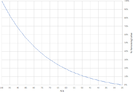
Asset value was assumed to depreciate linearly with respect to age, but given that PCR condition ratings decline in a non-linear manner, the overall relationship between condition and percent value remaining was non-linear as well. The Southwestern DOT used data from its pavement management system to establish a relationship between PCR and percent of life remaining, shown in the curve displayed in Figure B-2.1 below. The end of life based on condition was defined as a PCR value of 25.
Age-Based Approach
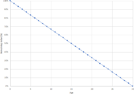
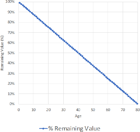
The age-based approach assumed linear depreciation by year, where the end of life for a pavement was defined as 30 years. Figure B-2.2 shows the curve representing the relationship between age and percent of value remaining for a given pavement section.
The Southwestern DOT used the curves to calculate remaining pavement value based on condition and age. In addition, the agency calculated a cost to maintain value and asset consumption ratio (ACR) for each approach. The calculations were performed in a spreadsheet tool where the agency could adjust parameters (e.g., cost, end-of-life criteria) to see the impacts on the results.
Results
Table B-2.1 details the calculation of asset value for the Southwestern DOT’s pavements. The table shows replacement value and remaining asset value based on two approaches for calculating depreciation: using the PCR rating; and using pavement age irrespective of condition. The results are summarized by whether or not the pavement is located on the National Highway System (On NHS, Off NHS).
Table B-2.1 Asset Value Results
| NHS | Replacement Value ($M) | Remaining Asset Value by Method ($M) | ACR by Method | Cost to Maintain by Method ($M) | |||
|---|---|---|---|---|---|---|---|
| Condition | Age-Based | Condition | Age-Based | Condition | Age-Based | ||
| On | 21,605 | 6,300 | 6,264 | 29.2% | 29.0% | 254 | 720 |
| Off | 36,369 | 6,814 | 6,532 | 18.7% | 18.0% | 427 | 1,212 |
| Total | 57,974 | 13,114 | 12,797 | 22.6% | 22.1% | 681 | 1,932 |
Lessons Learned
Lessons learned from the Southwestern DOT’s experience in comparing condition and age-based depreciation approaches for pavement asset valuation include:
- Using condition and age-based depreciation approaches for pavement can yield different remaining asset value results. An agency should carefully consider which approach is most appropriate to meet its needs.
- The basic differences between the approaches are easily understood. The age-based approach typically yields a lower remaining asset value. This approach does not account for
- In addition, the Southwestern DOT’s cost to maintain value was lower for the condition approach than for the age approach. The lower cost for the condition approach compared to the age approach is to be expected, given that the condition approach modeled an effective end of life at 81 years, while the age approach assumed an end of life at 30 years.
- Setting key parameters has a big impact on the results. Parameters should be set to reflect current management practices and adjusted as needed.
- For example, changing the pavement end of life for the Southwestern DOT from 30 years to 40 years would double the remaining value from $12.8 billion to $24 billion.
work performed on pavements to extend their life; if a pavement is near the end of its life, it has a relatively low value, regardless of its condition.
B-3. Calculating Asset Value for Assets with Varying Levels of Data Availability in a Western Agency
Summary
In this case study, a state department of transportation in the West, labeled the “Western DOT,” developed a tiered approach for calculating asset value for assets with varying levels of data availability. The agency, which includes numerous asset types beyond pavement and bridge in its asset valuation program, adjusted the calculation approach depending on the available data, allowing for a clearly defined and repeatable process.
Background
The Western DOT has two primary drivers for calculating and reporting asset value:. The first is to comply with the Federal Highway Administration’s (FHWA) requirement that State DOTs include a calculation of the value of National Highway System (NHS) pavement and bridge assets in their transportation asset management plans (TAMPs), and that they calculate the cost of maintaining asset value (23 CFR § 515.7(d)(4)). The second is to communicate asset value to the state legislature using an asset register (also included in the TAMP) containing an inventory and valuation for 14 asset types, ranging from bridge and pavement to lighting and signs.
In the Western DOT’s previous asset registers, asset value was typically calculated using a replacement cost approach that did not consider age or condition of the assets and thus did not reflect depreciation of the assets. In addition, the calculation approach was not defined nor documented across the asset types, making it difficult to reproduce the results. The Western DOT decided to improve its asset valuation approach by developing and implementing a consistent methodology that meets the agency’s needs and reflects best practices.
Methodology
Data
Ideally, the Western DOT could calculate both a replacement value and a depreciated current value for all assets. However, based on available data, it was difficult to generate meaningful depreciated values for some assets. In recognition of the challenges presented due to differences in available data, observed deterioration behavior of the asset, and management approaches, the agency defined three different approaches that can be followed to calculate asset value, depending on the available data. At minimum, the proposed approaches allow for a consistent and repeatable calculation of replacement value. If sufficient data are available, a depreciated current value may also be calculated.
Comprehensive Data Approach
The comprehensive approach was the most advanced approach but required sufficient data to calculate a condition or age-based depreciation to estimate current value. The Western DOT used this approach for assets with the most mature management process and the most available data. The necessary data to use the comprehensive approach include:
- Complete asset inventory (or random, representative sample of the data)
- Unit replacement cost
- Residual value (the value of an asset when it is fully depreciated)
And
- Age-based depreciation
- Useful life (the age at which an asset is fully depreciated)
- of assets exceeding useful life
- Average age of assets that have not exceeded the useful life
Or
- Condition-based depreciation
- Condition scale (the condition at which an asset is fully depreciated)
- of assets in each condition state
- life remaining at each condition state
Moderate Data Approach
For assets with some inventory data but no age or condition data, it was not feasible to calculate a depreciated current value. Instead, the Western DOT used a simplified approach to calculate replacement value. Assets with moderate data used available inventory and unit cost data to calculate replacement value. If complete inventory data were not available, a random and representative sample could be used instead.
Minimal Data Approach
For assets with minimal data, it was not feasible to calculate a depreciated current value and was a challenge to calculate replacement value. When inventory data were not available, the Western DOT performed an analysis of available construction cost data and calculated an estimate of replacement value based on the extent of the road network, measured in centerline miles. This was a general approach that could be modified depending on the particular asset. The agency considered environmental characteristics and roadway types when choosing the scope of the road network to evaluate.
Results
After defining the calculation approaches, the Western DOT assigned and implemented an approach to each asset type depending on available data. Table B-3.1 details the calculation of asset value for the Western DOT’s assets, organized by calculation approach. The table shows replacement value for all assets and remaining asset value where available.
Table B-3.1 Asset Value Results
| Calculation Approach | Depreciation Approach | Asset | Replacement Value ($M) | Remaining Value ($M) |
|---|---|---|---|---|
| Comprehensive Data Approach | Condition-based Non-linear | Bridge | 14,560 | 9,695 |
| Condition-based Linear | Pavement | 27,655 | 24,378 | |
| Signals | 482 | 321 |
| Culverts/Storm Drains | 2,503 | 7,217 | ||
| Barrier | 878 | 658 | ||
| Age-based Linear | Striping | 149 | 56 | |
| ITS | 829 | 603 | ||
| Signs | 975 | 435 | ||
| Lighting | 194 | 74 | ||
| Moderate Data Approach | None | Rumble Strip | 21 | Not calculated |
| Cattle Guard | 85 | |||
| Fence | 289 | |||
| Concrete Flatwork | 167 | |||
| Walls | 9,012 |
Lessons Learned
Lessons learned from the Western DOT’s experience in developing asset valuation approaches for varying levels of asset data include:
- Calculating asset value can be challenging for assets with less mature management processes and less available data
- Using simplified calculation approaches for different levels of data availability allows an agency to calculate asset value for a range of assets.
- The first step toward asset valuation is to evaluate the availability of data and select an approach: comprehensive data, moderate data, or minimal data. The minimal data approach may be the best approach for many assets that are trying to build maturity in asset valuation. This approach can help define a repeatable process for calculating replacement value on an annual basis. The approach can be updated for each asset if necessary as more data are made available.
- Having a defined, repeatable asset valuation process is important for building asset valuation maturity
- Repeating the calculation on a regular basis allows an agency to measure and compare progress over time. Without a consistent calculation approach, comparisons are less meaningful.
- While some assets may have data gaps, developing simple valuation approaches is possible. The initial effort of developing the valuation approach can help identify data gaps and make progress toward closing those gaps and improving the valuation approach.
B-4. Comparing Bridge Valuation Using Three Depreciation Approaches in a Northwestern Agency
Summary
In this case study, a state department of transportation (DOT) located in the Northwest, labeled the “Northwestern DOT,” calculated asset value for its bridges using three depreciation approaches to measure their remaining (current) value. In comparing the results from the composite condition rating, minimum condition rating, and age-based approaches, the Northwestern DOT was able to gain a more complete understanding of its bridge inventory and identify the desired calculation approach for the agency’s needs.
Background
The Northwestern DOT’s primary driver for calculating and reporting asset value is to comply with the Federal Highway Administration’s (FHWA) requirement that State DOTs include a calculation of the value of National Highway System (NHS) pavement and bridge assets in their transportation asset management plans (TAMPs), and that they calculate the cost of maintaining asset value (23 CFR § 515.7(d)(4)).
In past versions of its TAMP, the Northwestern DOT estimated asset value based on replacement cost alone, without accounting for the assets’ age or condition. As a result, depreciation was not reflected in the valuation. This method also did not provide a useful estimate for the cost required to maintain asset value, since preserving full replacement value was calculated at $0. To enhance the accuracy and relevance of its asset valuations, the Northwestern DOT explored three depreciation-based approaches aimed at determining both the remaining value of bridges, and the cost necessary to sustain that value.
Methodology
Data
The Northwestern DOT used age and condition data from the National Bridge Inventory (NBI) to calculate asset value. For the age-based approach, each bridge’s value was calculated as a whole, while the condition-based approaches split each bridge into their three major components (deck, superstructure, substructure).
Condition-Based Approaches
While the relationship between the age of a bridge and its percent value remaining is assumed to be linear, bridges typically exhibit a non-linear relationship between condition and percent value remaining. The Northwestern DOT used data from a “do-nothing” scenario in the FHWA Bridge Investment Program (BIP) tool to develop deterioration curves for bridges within their jurisdiction based on component condition. The agency developed deterioration curves for each bridge component, as well as a “minimum component” deterioration curve based on the minimum component rating of a bridge. The end of life was defined as a component rating of 3.
Composite Component Rating Approach
The first approach tested by the Northwestern DOT was the composite component rating approach, in which the agency calculated the percent remaining value for each bridge component using the modeled deterioration curves. Those percentages were combined in a weighted average based on defined parameters
(20% deck, 40% superstructure, and 40% substructure) to obtain a composite percent value remaining for the entire bridge.
Minimum Component Rating Approach
The second approach was the minimum component rating approach, which used the lowest component condition rating of a bridge to define the effective age of the bridge.
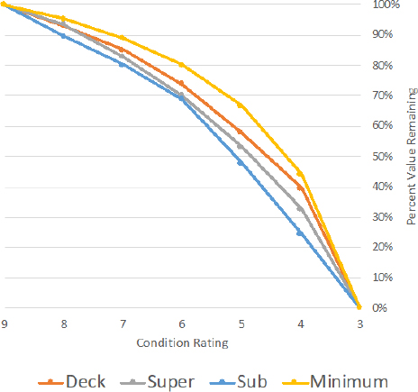
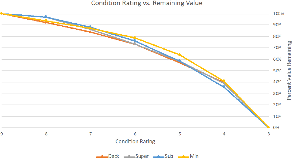
Figure B-4.1 shows the relationship between condition ratings and remaining value for each bridge component as well as for the minimum component. Note that the results shown for culverts are the same as that for substructure, as the agency found that culverts behaved similarly to substructures, but that there was not enough data for culverts to calculate a deterioration curve.
Age-Based Approach
The Northwestern DOT also used the typical bridge useful life to calculate an age-based valuation for each bridge. This method assumed linear depreciation by year, where the end of life for a bridge was set at 80 years and bridge age was defined by identifying the more recent of year built or year reconstructed. Figure B-4.2 shows the curve representing the relationship between age and percent of value remaining for a given bridge.
The Northwestern DOT used the curves to calculate remaining bridge value based on each approach. The agency also calculated a cost to maintain value and asset consumption ratio (ACR) for all three methods. The calculations were performed in a spreadsheet tool where the agency could adjust parameters including unit replacement cost, end-of-life criteria, component weightings and condition rating thresholds. This tool allowed the agency to explore the impact of these parameters on the results.
Results
Table B-4.1 summarizes the calculation of asset value for the Northwestern DOT’s bridges. The table includes replacement value as well as the remaining asset value based on the three approaches for calculating depreciation: using a weighted average of all three major components condition ratings, using the condition
data of each bridge’s most degraded component, and using bridge age irrespective of condition. While the detailed results are available by owner (State DOT, Other), the case study results summarize all NBI bridges in the state, organized by whether or not the bridge is located on the National Highway System (On NHS, Off NHS).
Table B-4.1 Asset Value Results
| NHS | Repl. Value ($B) | Remaining Asset Value by Method ($B) | ACR by Method (%) | Cost to Maintain by Method ($M) | ||||||
|---|---|---|---|---|---|---|---|---|---|---|
| Comp. Rating | Min. Rating | Age | Comp. Rating | Min. Rating | Age | Comp. Rating | Min. Rating | Age | ||
| State DOT | ||||||||||
| On | 45.3 | 34.1 | 29.6 | 22.5 | 75.3 | 65.3 | 49.6 | 871 | 1,118 | 552 |
| Off | 8.0 | 6.2 | 5.6 | 3.4 | 78.3 | 69.7 | 43.1 | 152 | 194 | 94 |
| Total | 53.3 | 40.3 | 35.1 | 25.9 | 75.8 | 66.0 | 48.6 | 1,023 | 1,313 | 646 |
| Other Owner | ||||||||||
| On | 5.6 | 4.1 | 3.5 | 2.9 | 73.4 | 64.0 | 53.0 | 107 | 138 | 61 |
| Off | 14.6 | 11.3 | 10.2 | 7.2 | 77.2 | 69.5 | 49.3 | 280 | 362 | 172 |
| Total | 20.2 | 15.4 | 13.7 | 10.2 | 76.2 | 68.0 | 50.3 | 387 | 500 | 233 |
| All | ||||||||||
| On | 50.8 | 38.2 | 33.1 | 25.4 | 75.1 | 65.2 | 50.0 | 978 | 1,256 | 613 |
| Off | 22.6 | 17.5 | 15.7 | 10.7 | 77.6 | 69.6 | 47.1 | 433 | 556 | 265 |
| Total | 73.4 | 55.7 | 48.9 | 36.1 | 75.9 | 66.5 | 49.1 | 1,410 | 1,812 | 878 |
Lessons Learned
Key takeaways from the Northwestern DOT’s comparison of age and condition-based depreciation approaches for bridge asset valuation are listed below:
- The approach chosen for calculating depreciation has a large impact on the end results. An agency should carefully consider which approach is most appropriate to meet its needs.
- The composite component condition approach typically yields a higher remaining value than the other approaches, as it considers the condition of each component of a bridge separately. This method accounts for the different characteristics of bridge components and allows the agency to adjust the weighting of each to match their standard practices.
- The minimum rating approach tends to yield lower valuations than the composite approach, as it uses the lowest component rating and assumes deterioration rates similar to that of the deck, typically the shortest-lived component. This approach also leads to a higher cost to
- Transportation agencies may select this approach to be conservative when calculating the value of their assets. Some bridge components are easier to repair or replace than others. For example, a bridge deck can be repaired or replaced relatively inexpensively, while a bridge substructure cannot be easily replaced without doing a full bridge construction.
- The age-based approach yields the lowest asset value, as it does not account for work performed on bridges to extend their life. A bridge that is beyond its useful life in age but has been well maintained and remains in good condition would have zero value remaining based purely on age.
- It is also essential that the parameters used in the calculations are consistent with the DOT’s real-world practices to get the most out of their calculation results.
- For example, the components in the composite approach should be weighted based on state-specific data and/or engineering judgment. Likewise, the definition of end of life should be aligned with current bridge management practices.
maintain value compared to the composite approach, due to shorter useful life calculated in the model.
B-5. Using FHWA BIP Tool Data to Develop Bridge Deterioration Curves
Summary
As part of NCHRP Project 20-44(46), the research team used data from the Federal Highway Administration’s (FHWA) Bridge Investment Program (BIP) tool to develop deterioration curves by component for bridges. The data includes all US states and offers a straightforward and repeatable approach to establishing a relationship between bridge condition and remaining value.
Background
Ideally calculations of bridge asset value should incorporate depreciation, or consumption of the value of a bridge asset. One approach for calculating depreciation is to observe a bridge’s current condition and then use a deterioration model to estimate the time until the bridge reaches its useful life. This analysis is typically performed by bridge component. Bridges typically have three components: the deck, superstructure and substructure, while bridge-length culverts have a single component, the culvert.
While all State DOTs have bridge management systems that can be used to estimate useful lives of bridge and culvert components, in practice the calculation can be cumbersome to perform. This case study provides an approach for making the depreciation calculation using state-specific data compiled by FHWA.
Data
The FHWA BIP is a competitive discretionary funding program for improving bridge condition as well as safety and reliability. The BIP includes data on expected deterioration for each bridge in the National Bridge Inventory (NBI). This was compiled by performing model runs in FHWA’s National Bridge Investment Analysis System (NBIAS). Data obtained from NBIAS to support the BIP includes predicted component ratings for each bridge and bridge-length culvert in the NBI over a fifty year time horizon, broken up into five year periods.
Methodology
The team defined the following process for using the data in the BIP to develop bridge component depreciation curves for a given state:
- The first step is to compile BIP data for the selected state. The BIP data detail the predicted time to deteriorate (in number of 5-year periods) from current conditions to each component condition and from the minimum component condition given no work is performed on the bridge.
- The next step is to calculate the average decline in component condition per period for each component for each bridge.
- Next it is necessary to calculate the average annual condition drop for each component by initial rating value (0-9). This is accomplished by weighting each bridge by deck area to account for size and dividing the first (five year) period drop by five to get an annual average.
- The next step is to use the average annual condition drop to determine the average time required to deteriorate to each rating value starting from new condition.
- Finally, the depreciation curve is calculated by establishing the percent of value remaining at each rating value for each component. This is calculated by subtracting from 100% the ratio of time to deteriorate to the rating value to the time to reach the end of life (e.g., a rating of 3).
- In conjunction with bridge inventory data and unit cost data, the resulting deterioration curves can be used to calculate a remaining asset value.
Results
Figure B-5.1 below provides an example calculation of the percentage of asset value remaining for each of the components of a bridge, as well as for the minimum component rating. As shown in the figure, a component is assumed to have reached the end of its useful life if its rating is 3 or less. The minimum component condition rating approach uses the lowest component condition rating to define the effective age of the bridge. Note this is an example set of curves: the process can be repeated to obtain state-specific curves.
Lessons Learned
Key takeaways from the development of an approach for developing bridge deterioration curves in support of asset valuation are listed below:
- When attempting to define the relationship between bridge condition and remaining value, observed deterioration curves can be developed using FHWA BIP data in the absence of readily available defined deterioration curves.
- State DOTs typically have existing bridge deterioration curves; however they may be embedded in management systems and difficult to extract, or a state may have many deterioration curves for families of bridges. The work described in the pilot offers a simplified approach to deriving deterioration curves for state bridges by component, and thus a path toward calculating a depreciated current asset value.
- The approach should be adjusted to meet an agency’s needs and/or data.
- For example, a state may find that culverts behave similarly to substructures, but that there is not enough data for culverts to calculate the time to deteriorate to each rating value. In this case, it is acceptable to use a substitute curve, such as the one for substructures, to represent the relationship between culvert condition and remaining value.
B-6. Valuing a Bridge Using the Economic Perspective in an Eastern Agency
Summary
In this case study, a state-wide transportation agency in an eastern state, labeled the “Eastern DOT,” calculated the value of an existing bridge by determining the remaining user and social benefits of the structure. By comparing the anticipated lifecycle benefits with and without the bridge, Eastern DOT was able to determine the transportation and social value of the bridge to the traveling public and justify ongoing investments to keep it in good condition.
Background
Eastern DOT’s primary driver for calculating and reporting asset value is to comply with the Federal Highway Administration’s (FHWA) requirement that State DOTs include a calculation of the value of National Highway System (NHS) pavement and bridge assets in its transportation asset management plans (TAMPs). In prior TAMPs, Eastern DOT employed a condition-based depreciation approach based on replacement costs to understand and report asset values. However, this approach does not evaluate or communicate the value these assets provided to the public or the potential transportation or social loss that could result from failure to upkeep the assets. Eastern DOT decided to supplement its calculation methodology by testing an economic value-based approach for calculating the economic value of a bridge to the public.
Methodology
Data
Eastern DOT first determined traffic routing impacts in the absence of the bridge and then estimated future volumes and travel distances and times both with and without the facility. Starting with current volumes on the current and alternative routes, Eastern DOT computed the loss of demand due to congestion and assembled an inventory of travel times “with” and “without” the bridge. This inventory included motor vehicle traffic (car and light, medium, and heavy truck) and active transportation trips. The transportation data was supplemented with economic valuation estimates based on US Department of Transportation (USDOT) and Environmental Protection Agency (EPA) guidance.
Economic Value Approach
Eastern DOT assumed that the economic value equals the lifecycle benefits to users of having the asset in place and in good working condition. To determine these benefits, Eastern DOT calculated the travel time loss associated with the alternative routing required without the facility, including the loss to existing users of the replacement route who would face added congestion with additional traffic, the additional costs of operating vehicles along longer, more congested routes, the change in crashes expected due to the net change in vehicle-miles traveled (VMT) caused by the longer, slower route, changes in emissions, loss of mobility for those current trip makers who could be expected to avoid trip-making due to the longer, slower routing, and loss of bicycle trip access. There may be further disruptions or changes in the economy. These were not considered in the economic value approach, which focused only on the direct impacts.
Eastern DOT valued these impacts using USDOT and EPA estimates of travel time and costs, mobility value, costs of crashes by type, and the value of active transportation options. The net value of travel and emissions was calculated for both the “with” and “without” bridge cases over a thirty-year forecast. The future benefits were discounted based on USDOT guidance for an appropriate discount rate and then summed for each case. The Eastern DOT compared the total benefits of each case to estimate a loss that occurs in the “without” bridge case to determine its net present user and social value.
Results
Table B-6.1 details the estimated user and social value by benefit category for both a current dollar and discounted dollar perspective. Consistent with USDOT guidance, the Eastern DOT applied a 3.1 percent discount rate, except for CO2 which was discounted at 2.0 percent (also per USDOT guidance). The discounted dollar estimate is the better economic value of the bridge.
Table B-6.1 Asset User and Social Value Results
| Impact Category | Over the Project Lifecycle | |
|---|---|---|
| Constant Dollars | Discounted Dollars | |
| Costs of Additional Travel Time | $9,670.0 | $5,914.7 |
| Additional Vehicle Operating Costs | $846.4 | $522.9 |
| Safety Costs | $331.7 | $205.3 |
| Total Emission Costs | $153.6 | $109.6 |
| Loss of Mobility Value | $119.3 | $73.0 |
| Lost Bicycle Route Benefits | $0.01 | $0.007 |
| Total Bridge Value | $11,121.1 | $6,825.7 |
Lessons Learned
Lessons learned from the Eastern DOT’s experience in developing an economic value-based approach for bridge asset valuation include:
- Consideration of the travel impacts of the “without” case is crucial to understanding the facility valuation.
- The valuation approach applied utilizes speed-flow and elasticity of demand estimates to calculate future travel behavior.
- An approach utilizing a travel demand model might result in more defendable estimates.
- Economic valuation of assets is not widely understood but travel benefits are easily grasped by policy makers who intuitively understand the public benefits associated with their assets.
- As a result, an economic valuation is useful for justifying investments to maintain assets over a life cycle.
- Future improvements to this case study could include using a travel demand model to estimate more precise rerouting travel impacts that may occur with and without the bridge.
- In addition, the estimated asset value reflects the operating conditions of the structure (e.g., traffic volumes and speeds experienced by users), but it does not consider asset deterioration. A variant of this approach could adjust the economic valuation using a measure of asset condition such as a bridge health index.
B-7. Valuing Pavement Based on Condition in a Metropolitan Agency
Summary
In this case study, a metropolitan transportation agency, labeled the “Metropolitan TA,” calculated asset value for its pavements using a condition-based depreciation approach to calculate value. The agency was able to use calculated asset value to help justify ongoing pavement maintenance investments.
Background
The Metropolitan TA’s primary driver for calculating and reporting asset value is to demonstrate the value of a targeted pavement investment program. The calculated asset value also is consistent with the Federal Highway Administration’s (FHWA) requirement for State DOTs to include a value of National Highway System (NHS) pavement and bridge assets in their transportation asset management plans (TAMPs), and that they calculate the cost of maintaining asset value (23 CFR § 515.7(d)(4)). The Metropolitan TA is interested in similar methodologies for its own TAMP.
In the Metropolitan TA’s previous TAMPs, asset value was calculated using a replacement cost approach that did not consider age or condition of the assets and thus did not reflect depreciation of the assets. Also, the calculation did not yield a meaningful estimate of the cost to maintain asset value, since the cost to maintain replacement value was $0. The Metropolitan TA decided to improve its calculation methodology by testing a condition-based depreciation approach for calculating remaining asset value and the cost to maintain asset value.
Methodology
Data
The Metropolitan TA used a pavement condition index (PCI) based on pavement distress observations to categorize the condition of, and to manage its pavements, collected for each management section on the network. Pavement asset value was calculated for the pavement both on and off the NHS and then aggregated. Data was collected for 2017, 2019, 2021, and 2023 to support value trend analysis.
Condition-Based Value Approach
Asset value was assumed to depreciate relative to an estimated perfect condition value computed from cost-to-replace estimates specific to on- and off-NHS treatment requirements. This baseline value was computed for all pavements inclusive of bike lanes and parking areas. The PCI captured in the Metropolitan TA’s pavement inventory system was then used to depreciate the value to a condition-based value. This exercise was repeated for each year of the analysis to assess trends in valuation. Then a cost to improve to full value was estimated to compare the valuation trend to the condition-based valuation.
The Metropolitan TA used valuation estimates to assess the impact of its pavement condition investment program. In addition, the agency calculated a cost to improve value across the whole of the network. The calculations were performed in a spreadsheet tool where the agency could adjust parameters (e.g., cost to improve and maintain) to see the impact on the results.
Results
Table B-7.1 details the calculation of the current condition-based asset value for the Metropolitan TA’s pavements. The table shows replacement value and remaining asset value based on the PCI estimate as well as the cost to maintain based on PCI-specific treatment costs for on- and off-NHS pavements. The results are summarized by pavement location relative to the National Highway System (On NHS, Off NHS).
Table B-7.1 Asset Value Results
| NHS | Replacement Value ($M) | Remaining Asset Value by PCI Method ($M) | Cost to Maintain ($M) |
|---|---|---|---|
| On | $707.3 | $624.4 | $26.2 |
| Off | $2,536.9 | $1,951.3 | $219.6 |
| Total | $3,244.2 | $2,575.8 | $245.8 |
Lessons Learned
Lessons learned from the Metropolitan TA’s experience in developing a condition-based depreciation approach to pavement asset valuation include:
- Using condition-based depreciation approach is useful for justifying an investment in condition improvement and for assessing valuation over time.
- The valuation approach sets alternatives for asset maintenance on a common valuation system and is useful for communicating the scale of both value and potential loss when determining an investment strategy.
- A time-based comparison of valuations mixes deterioration and improvement in a way that can be challenging to communicate unless carefully delineated.
- The cost-to-maintain parameter has a significant impact on the results. Costs change over time and retrospective analysis should consider the impact of both practice and inflation over time. Future valuation should be adjusted as needed.
- Future enhancements could include comparisons of the change in asset valuations to the investments in the pavement program, while considering the yearly deterioration in pavement condition.
B-8. Calculating Vehicle Asset Value Using the Market Perspective
Summary
In this case study, the research team calculated developed a depreciation curve for cutaway buses using the market perspective to estimate current asset value. In comparing the results obtained using market value with those obtained by applying a linear, age-based depreciation curve to replacement value, the research team found the market value provides a different, and potentially more accurate calculation of asset value.
Background
Calculations of asset value should ideally incorporate depreciation, or consumption of the value of an asset. Where a market exists for resale of an asset the effect of depreciation is directly measurable: it is the difference between the purchase price of a new asset and the resale value of a used one. Where no such market exists, it is necessary to calculate depreciation through other means. The most straightforward approach for doing so it to establish the useful life of an asset and then assume straight-line depreciation as a function of age.
This case study provides an example of how the market value can be used to help establish asset value. In this example the research team established market values for used assets for a particular asset class, cutaway buses, and then derived a depreciation curve from the market data.
Methodology
Data
In its National Transit Database (NTD) the Federal Transit Administration (FTA) defines a “cutaway bus” as “A vehicle in which a bus body is mounted on the chassis of a van or light-duty truck. The original van or light-duty truck chassis may be reinforced or extended. Cutaways typically seat 15 or more passengers, and typically may accommodate some standing passengers…”1 In the United States thousands of transit agencies rely on cutaways for transit and paratransit service. As shown in Table B-8.1, FTA estimates that the useful life of a cutaway is approximately 10 years.2
___________________
1 Federal Transit Administration (FTA). National Transit Database Glossary. FTA, 2025. Accessed at the following URL on July 24, 2025: www.transit.gov/ntd/national-transit-database-ntd-glossary#C
2 FTA. Default Useful Life Benchmark (ULB) Cheat Sheet. FTA, 2021.
Table B-8.1 Default Useful Life Benchmarks for Transit Vehicles
| Vehicle Type | Default ULB (years) | Vehicle Type | Default ULB (years) |
|---|---|---|---|
| Articulated bus | 14 | Minivan | 8 |
| Automated guideway vehicle | 31 | Commuter rail locomotive | 39 |
| Automobile | 8 | Commuter rail passenger coach | 39 |
| Over-the-road bus | 14 | Commuter rail self-propelled passenger car | 39 |
| Bus | 14 | School bus | 14 |
| Cable car | 112 | Steel wheel vehicles | 25 |
| Cutaway bus | 10 | Streetcar | 31 |
| Double decked bus | 14 | Sport utility vehicle | 8 |
| Ferryboat | 42 | Trolleybus | 13 |
| Heavy rail passenger car | 31 | Trucks and other rubber tire vehicles | 14 |
| Inclined plane vehicle | 56 | Aerial tramway | 12 |
| Light rail vehicle | 31 | Van | 8 |
| Monorail vehicle | 31 | Vintage trolley | 58 |
Given the large inventory of cutaway vehicles, and the fact that a vehicle may be readily transferred from one owner to another, a well-defined market exists for resale of cutaway buses. Thus, the research team selected the cutaway bus as an example asset to use to illustrate calculation of asset value using a market perspective.
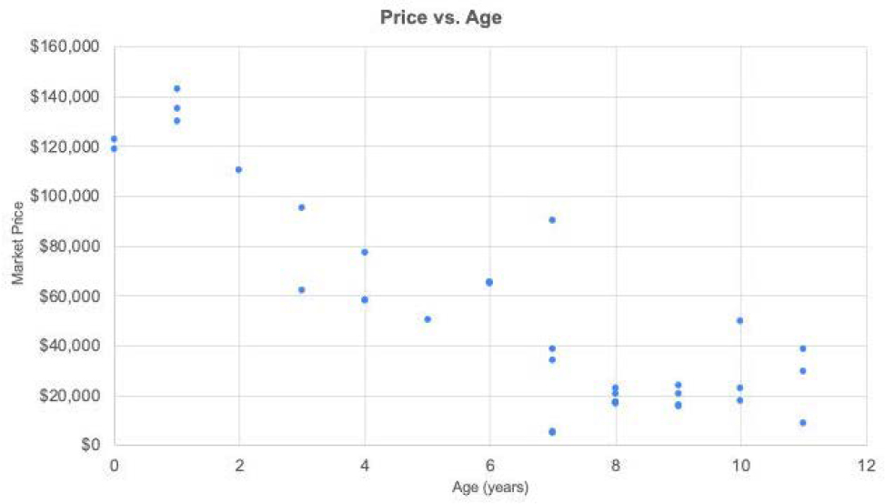
To establish market value for cutaways the team first selected a common cutaway configuration, specifically cutaways configured for passenger service using a Ford E450 chassis. The research team then queried six different publicly available systems for resale of vehicles. Four of the six systems list prices for vehicles, and two offer vehicles for auction. For the auction-based systems the team relied on completed sales rather than requested prices. Figure B-8.1 is a scatter plot showing prices as a function of vehicle age established in this step. As illustrated in the figure, data were collected for 34 vehicles that range in age from 0 to 11 years. Prices were found to vary from $4,650 to $142,725. The team tested the correlation between price and both age and mileage but found a stronger correlation between price and age than between price and mileage.
Depreciation Curve Development
The team next calculated a depreciation curve for cutaway vehicles by fitting an exponential curve to the data. The equation of the curve showing the relationship between age and price is as follows:
Where P is the price of a vehicle with age t and a and b are parameters fit from the data. The best-fit curve has an R-squared value of 0.81, which indicates a reasonable correlation between the age and price.
The resulting curve predicts market value as a function of age. The curve may be restated to predict value as a percent of new vehicle cost by dividing all values by the parameter a (calculated as $132,701 for this dataset). The equation of the best-fit curve recast in this fashion is:
Where V is the remaining value as a percent of a new vehicle cost at age t.
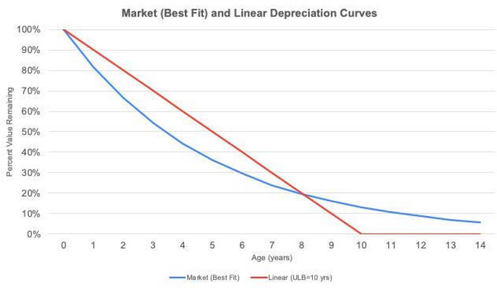
The research team also calculated a simplified depreciation curve assuming straight-line depreciation from 0 to 10 years. Figure B-8.2 shows the two alternative depreciation curves. Compared to the straight-line depreciation approach, the best-fit curve fit based on market values shows accelerated depreciation for ages less than eight years. This behavior is consistent with typical vehicle pricing on the open market experienced by consumers: a new vehicle loses value quickly after its purchase but holds some value for a number of years.
Illustrative Example
As an illustration of the approach, assume there is a transit agency with a fleet of cutaways evenly distributed in age from 0 to 10 years. In this fleet, the average age of a cutaway would be 5 years. Using the linear depreciation approach, the average remaining value of a vehicle would be 50% of the value of a new vehicle based on the assumption of straight-line depreciation. By contrast, based on market value the average remaining value would be 44% of the value of a new vehicle. This result may be obtained by calculating value for each age from 0 to 10 years and averaging the result. Thus, in this case using market value results in value that is approximately 12% lower than that estimated using straight-line depreciation.
However, if the fleet of cutaways had an even age distribution between 6 and 14 years, the average remaining value of a vehicle would be calculated as approximately 11% of new vehicle cost using straight-line depreciation and 15% using market value. In this case, the market value depreciation curve yields a higher remaining value for the vehicles. A summary of example scenarios is included in Table B-8.2.
Table B-8.2 Example Applications of Market Value and Linear Depreciation Approaches
| Fleet Age Distribution (years) | Vehicle Unit Repl. Value ($) | Market Value Approach | Linear Depreciation Approach | ||
|---|---|---|---|---|---|
| Avg. Remaining Value by Vehicle ($) | Avg. Remaining Value by Vehicle (%) | Avg. Remaining Value by Vehicle (%) | Avg. Remaining Value by Vehicle (%) | ||
| 0 to 10 | 132,701 | $58,441 | 44% | $66,351 | 50% |
| 6 to 14 | $19,748 | 15% | $14,745 | 11% | |
Lessons Learned
Conclusions drawn from this case study include the following:
- For an asset for which a market exists, it is possible to calculate depreciation using the market perspective.
- Calculating asset value using the market perspective can be a challenge for many transportation assets because a market for resale of culverts, overhead signs, bridges, and guardrail hardly exists. However, in the case where a market does exist, such as for vehicles, asset price data from sales on the open market can be used to develop a depreciation curve for a given asset.
- The depreciation curve resulting from the market perspective may differ significantly from a simple linear depreciation approach.
- A vehicle’s price on the market theoretically represents all the available information about the asset, such as any treatments performed on the asset and the condition of the asset. Thus, the vehicle’s price may better represent the remaining value than its age, particularly as a vehicle approaches its typical useful life. A depreciation curve based on market values may yield higher remaining value for older vehicles relative to a straight-line depreciation approach, while the opposite may be true for newer vehicles.
B-9. Valuing Highway Assets Using the Economic Perspective in a Western Agency
Summary
In this case study, the state department of transportation in a Western state, labeled “Western DOT,” calculated the value of an existing highway by determining the remaining user and social benefits of the facility. By comparing the anticipated life-cycle benefits with and without the highway, Western DOT was able to determine the transportation and social value the highway provides to the traveling public and businesses, helping to justify ongoing investments to keep it in good condition.
Background
Western DOT’s primary driver for calculating and reporting asset value was to comply with the Federal Highway Administration’s (FHWA’s) requirement that State DOTs include a calculation of the value of National Highway System (NHS) pavement and bridge assets in its transportation asset management plan (TAMP). In prior TAMPs, Western DOT employed a straight-line depreciation approach based on investment costs to understand and report asset values. However, this approach does not evaluate or communicate the value these assets provide to the public or the potential transportation or social loss that could result from failure to upkeep their assets. The highway selected for evaluation is a significant freight corridor and failure to upkeep would likely carry economic consequences beyond the vehicles and drivers on the road. The value to the economy is not captured under their traditional approach to asset valuation. Western DOT decided to supplement its calculation methodology by testing an economic value-based approach to estimate the highway’s economic value to the public.
Methodology
Data
Western DOT first determined freight and passenger traffic routing impacts in the absence of the highway and then estimated future volumes, travel time and distances both with and without the facility. Starting with current volumes derived from weigh station counts on both the existing and alternative routes and modes, Western DOT computed mode shifts and loss of demand due to changes in travel time and costs and assembled a comparative inventory of travel times “with” and “without” the highway. This inventory included freight motor vehicle traffic, personal vehicle traffic, and freight movements associated with non-highway modes. The transportation data was supplemented with economic valuation estimates based on US Department of Transportation (USDOT), Western DOT studies, public data on freight movement costs and times, and US Department of Energy (US DOE) guidance.
Economic Value Approach
Western DOT assumed that the highway’s economic value corresponds to the life-cycle benefits it provides to users and freight shippers when the asset is in place and maintained in good working condition. To determine these benefits, Western DOT calculated the travel time loss and additional costs associated with the alternative routing required without the facility. Additionally, Western DOT considered increased costs to shippers associated with quicker but more costly shipping times, changes in crash rates due to the net change in vehicle-miles traveled (VMT) as a result of the anticipated freight mode shifts and personal travel trip-
making reductions, changes in emissions, loss of mobility for current trip makers who could be expected to avoid trip-making due to the loss of access. There may be further disruptions or changes in the economy. These were not considered in the economic value approach, which focused only on the direct impacts.
Western DOT valued these impacts using USDOT and EPA estimates of travel time and costs, data on the economic cost of delay in freight movements from the academic literature, costs of crashes by type, and the value of GHG emissions. The net value of travel and emissions was calculated for both the “with” and “without” highway scenarios over a thirty-year forecast. The future benefits were discounted based on USDOT guidance for an appropriate discount rate and then summed for each case. The Western DOT compared the total benefits of each case to estimate a loss that occurs in the “without” highway case to determine its net present user and social value.
Results
Table B-9.1 details the estimated user and social value by benefit category for both a current dollar and discounted dollar perspective. Consistent with USDOT’s 2024 guidance, the Western DOT applied a 3.1 percent discount rate, except for CO2 which was discounted at 2.0 percent (also per USDOT guidance). The discounted dollar estimate is the better economic value of the highway.
Table B-9.1 Asset User and Social Value Results, in millions
| Impact Category | Over a 30-Year Project Life cycle | |
|---|---|---|
| Constant Dollars | Discounted at 3.1% | |
| Costs of Additional Travel Time | $2,768.6 | $1,729.1 |
| Additional Vehicle Operating Costs | $23,732.7 | $14,821.7 |
| Commodity Delay Cost | -$10,370.9 | -$6,479.9 |
| Total Emission (GHG) Costs3 | $16,009.1 | $11,454.5 |
| Safety Costs | -$342.8 | -$214.5 |
| Total Benefits | $31,789.5 | $21,306.5 |
Lessons Learned
Lessons learned from the Western DOT’s experience in developing an economic value-based approach for highway asset valuation include:
- For freight corridors, it is essential to consider not only alternative routes, but also alternative modes of transport, assuming that shippers will find a way to move freight regardless of cost.
- For alternative freight modes, there can be a trade-off between time and cost, and both need consideration in order to accurately quantify the net value of the facility.
- Shippers’ behavior in the absence of the highway was estimated for this case study based on data from before the opening of the highway, but also from data covering a prior closure due to flooding.
- Prior event data can be useful for estimating behavior in an alternative scenario.
___________________
3 The environmental discount rate for CO2 within the Emission calculations is 2.0%. as per the USDOT BCA Guidance.
- Future improvements to this case study could include using a multi-modal travel demand model to estimate more precisely the rerouting travel impacts that may occur with and without the highway.
- This might also include a consideration of emerging freight delivery technologies (such as drones and pilotless aircraft) and their impact on the decision-making for rerouting.
- Economic valuation of assets is not widely understood but travel benefits are easily grasped by policy makers who intuitively understand the public benefits associated with their assets.
- As a result, an economic valuation is useful for justifying investments to maintain assets over a life cycle.
- In addition, the estimated asset value reflects the operating conditions of the structure (e.g., traffic volumes and speeds experienced by users), but it does not consider asset deterioration. A variant of this approach could adjust the economic valuation using a measure of asset condition such as a pavement condition index.


