Developing a Guide for Rural Highways: Reliability and Quality of Service Evaluation Methods (2024)
Chapter: Appendix C: Arterial Signal Spacing for Coordination
Appendix C: Arterial Signal Spacing for Coordination
If it has been determined that a stretch of roadway should be analyzed as an arterial (i.e., urban street), and that stretch of roadway includes two or more signalized intersections, a key question is whether signal coordination should be considered in the analysis of that arterial.
For background, the current guidance provided in the HCM7 regarding when to apply the Urban Streets analysis methodology (Chapter 16) is as follows:
The methodologies described in this chapter are typically used to evaluate an entire facility; however, for some specific conditions it may not be necessary to evaluate the entire facility. For these conditions, the appropriate segment or intersection chapter methodology may be used alone to evaluate selected segments or intersections. In general, it is up to the analyst to determine the spatial scope of each analysis (i.e., one intersection, one segment, two segments, or all segments on the facility) on the basis of analysis objectives and agency directives.
One condition for which it may be acceptable to evaluate an individual segment or intersection occurs when the segment or intersection is considered to operate in isolation from upstream signalized intersections. A segment or intersection that is effectively isolated experiences negligible influence from upstream signalized intersections. Flow on an isolated segment or at an isolated intersection is effectively random over the cycle and without a discernible platoon pattern evident in the cyclic profile of arrivals. These characteristics are more likely to be found when (a) the nearest upstream signalized intersection is sufficiently distant from the subject segment or intersection and (b) the subject segment or intersection, if signalized, is not coordinated with the upstream signal.
A segment or intersection is sufficiently distant from the nearest upstream signal if an intermediate intersection uses stop or yield control to regulate through traffic on the facility. If there is no intermediate STOP- or YIELD-controlled intersection, then Exhibit 16-2 can be used to obtain an indication of whether a segment or intersection is sufficiently distant from an upstream signal. If the distance between signals is above the trend line, then the subject intersection or segment is likely to operate as effectively isolated (provided that it is not coordinated with the upstream signal).
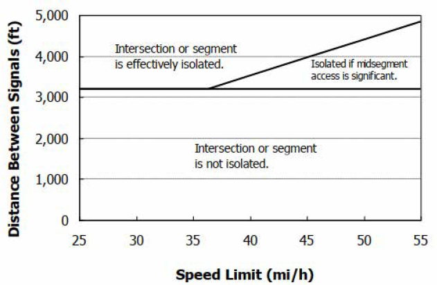
Source: HCM, Exhibit 16-2
If the roadway consists of a series of signalized intersections and coordination is employed and other traffic and roadway characteristics are conducive to maintaining favorable signal progression, the urban streets analysis methodology should be employed. Favorable signal progression implies that the proportion of vehicles arriving on the green signal indication (PVG) is higher than the effective green-to-cycle length (g/C) ratio. A proportion of vehicles arriving on green (PVG) value approximately equal to the g/C ratio is expected for random vehicle arrivals. This concept is illustrated in Figure C-2, with the g/C ratio for the example urban street configuration set to 0.5 (horizontal line).
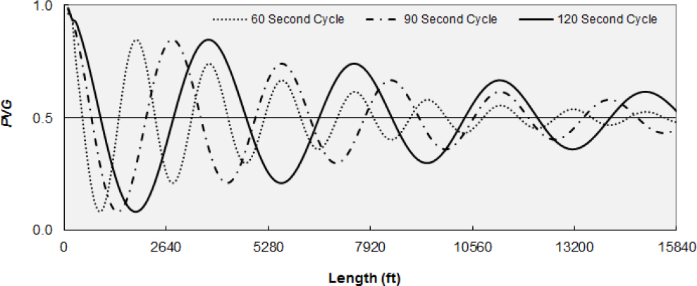
Source: Principles of Highway Engineering and Traffic Analysis, 7th Edition, Mannering and Washburn, Wiley & Sons, 2019.
Signal coordination and platoon dispersion are the primary factors affecting the difference between the g/C ratio and the PVG. Of course, even optimal signal coordination settings will offer no benefit when upstream platoons become highly dispersed before arriving at a downstream signal. The distance between the signals is generally the most influential factor on platoon dispersion, but other factors such as a high truck percentage and intermediate driveways may also be influential.
An experimental design was developed to investigate the question “At what point does platoon dispersion result in the PVG being equal to the g/C ratio?” This experimental design consisted of running the HCM urban streets methodology on arterial configurations with combinations of the variable values shown in Table C-1. Although some combinations may be not realistic (e.g., short intersection spacing and high posted speed limit), they are not problematic for analysis purposes, and thus were not filtered from the data set.
Table C-1. Urban Street Determination Experimental Design
| Variable | Levels |
|---|---|
| Traffic volume-to-capacity ratio | 0.40, 0.52, 0.64, 0.76 |
| Intersection Spacing (ft) | 660, 1320, 1980, 2640, 3300, 3960, 4620, 5280 |
| Heavy Vehicle % | 6, 12, 18 |
| Posted Speed (mph) | 30, 35, 40, 45, 50 |
| Total combinations: 4 × 8 × 3 × 5 = 480 | |
Arterial configuration
- The test arterial was composed of five intersections and four segments.
- All scenarios level terrain
- Driveway density is a function of intersection spacing, 1 per 660 ft (8 per mile)
- Demand volume proportions.
- Minor Street Volume Ratio (total minor street volume relative to major street volume) = 0.40
- Major Street Directional Split = 0.50
- Mid-Segment Analysis Volume Ratio (total access point volume relative to peak direction of major street) = 0.125
- Proportion Left Turns at Major Intersection = 0.10
- Proportion Right Turns at Major Intersection = 0.10
- Proportion Left Turns at Access Point = 0.05
- Proportion Right Turns at Access Point = 0.05
The traffic v/c levels were achieved under the following intersection configuration and signal timing plan assumptions:
Intersection configuration
- Major street approaches: 1 exclusive left-turn lane, 1 through-only lane, 1 shared through/right-turn lane
- Minor street approaches: exclusive left-turn lane, 1 shared through/right-turn lane
Signal timing plan
- Protected left-turn phasing
- Four timing stages: (1) major street opposing left turns, (2) major street through/right-turn movements, (3) minor street opposing left turns, (4) minor street through/right-turn movements.
- Cycle length: 90, 100, 110, 120 seconds for low to high v/c ratios, respectively.
- Coordination offset = distance from first intersection (ft) / posted speed (ft/s) – 3 seconds
A regression analysis was performed for the dependent variable, difference between PVG and g/C ratio. A linear, exponential, and 3rd degree polynomial form were calculated. In all three cases, the only statistically significant variable was the intersection spacing, which was highly significant. Segment running time, a function of posted speed limit, is one factor in the platoon dispersion model, but if offset values are set accordingly, as was done in this experiment, it is expected that posted speed limit will not be a significant contributor to the dispersion of platoons. Although a revised heavy vehicle-grade adjustment factor (fHVg) for signalized intersection saturation flow rate was included in the HCM 6th edition, it still falls short of being sensitive enough to the impacts of higher percentages of commercial trucks in the traffic stream, as discussed in Ozkul and Washburn (2019). Additionally, the calculations for link running speed do not consider truck percentage or grade. As expected, intersection spacing was highly significant. There is a natural spreading of vehicles that occur, from their originally bunched state when departing from an upstream signal. Additionally, there are generally more access driveways, or minor intersections, for longer
distances between major intersections. In this experiment, the number of driveways was fixed at one every 660 ft.
The exponential and polynomial forms both provided a slightly better fit than the linear form, but with the exponential form, there is a sharp increase in delta value for very low segment lengths, which is somewhat unrealistic, and the polynomial form is less intuitive. Thus, just the linear form is presented here.
| [C-1] |
Where:
∆PVG_gC = Difference between PVG and g/C ratio
SegmentLength = distance between major intersections, in feet
The linear model fit, R2, is 0.45. This is a relatively weak fit. Including independent variables for driveway spacing and turning percentages would likely improve the model fit. However, this potentially increased level of model precision may not be justified for the increased data collection requirements, particularly for driveway turning volumes. Nonetheless, a follow-on experiment will be conducted to examine the sensitivity of these two additional variables.
Setting ∆PVG_gC equal to zero and then solving for SegmentLength yields a value of 3927 ft. This value is approximately ¾ of a mile in length (3960 ft). Thus, if the signalized intersections along the roadway are spaced at ¾ of a mile or greater, they should be considered isolated, in which case random arrivals can be assumed. Otherwise, signal progression should be considered.


