Methods for Assigning Short-Duration Traffic Volume Counts to Adjustment Factor Groups to Estimate AADT (2024)
Chapter: 2 Literature Review
CHAPTER 2. LITERATURE REVIEW
INTRODUCTION
This chapter provides a review of various AADT estimation methods available in the literature and presents relevant findings, strengths, and weaknesses, as well as an assessment of the methods based on several key elements. At the beginning of the project, the research team gathered foreign and domestic documentation from national, federal, state, local, and private agencies. To collect these documents, the research team used various information resources including the Transportation Research Information Database, the TRB publication catalog, Texas A&M University’s library services, and general online searches. Initially, more than 300 documents were gathered. Upon an initial screening of these documents, the research team selected over 100 documents to review.
For completeness, the review did not focus only on traditional methods of assigning SDCs to factor groups but also covered nontraditional AADT estimation methods such as statistical and machine learning (ML) methods that use alternative types of data (e.g., census and probe data). This holistic approach was necessary for two reasons: (a) to identify differences between traditional and nontraditional methods with respect to key elements such as AADT accuracy, interpretability of factor groups, data requirements, complexity, and applicability to lower functional classes; and (b) to identify potential influential factors and surrogates for AADT that could potentially be used as inputs to improve the assignment process. A categorization of the various AADT estimation methods is provided in the next section.
AADT ESTIMATION METHOD
The literature and the survey conducted in this project revealed that many transportation agencies have been estimating AADT using variations of a traditional method that Drusch introduced in 1966 (Drusch 1966). An improved version of this method is recommended by the Federal Highway Administration’s (FHWA) Traffic Monitoring Guide (TMG) (FHWA 2022). The traditional method includes four general steps:
- Step 1—Computation of adjustment factors for each CCS. This step involves calculating adjustment factors (e.g., 12 monthly factors [MFs], 84 monthly day-of-week factors [MDWFs], etc.) separately for each CCS.
- Step 2—Establishment of adjustment factor groups. This step is known as the grouping process and involves creating groups of CCSs that exhibit similar traffic patterns. The goal is to produce internally homogeneous and well-defined groups with easily identifiable characteristics that allow direct assignment of every SDC to a group. After the groups are developed, group adjustment factors are computed for each group.
- Step 3—Assignment of SDCs to factor groups. This step involves assigning each SDC to one of the factor groups created in the previous step (or alternatively assigning the appropriate group adjustment factors to each count).
- Step 4—Annualization of SDCs. The annualization, or factoring, step involves applying one or more temporal group adjustment factors to each SDC. Further, growth factors need to be applied if a count was taken in a year other than the year for which AADT is being estimated. Axle-correction factors are needed if the count is not a volume or a classification count but instead measures the number of axles (e.g., a single pneumatic tube measures the number of axles, not the number of vehicles).
The assignment process is the most critical part of the traditional AADT estimation method because the accuracy of the AADT estimates largely depends on whether the adjustment factor(s) applied to each SDC adequately capture the traffic variability at the location of the count (Gulati 1995). Potential ineffective assignment of group factors to SDCs may triple the AADT prediction error (Davis 1996). Sharma et al. (1996) found that the assignment step can affect the AADT accuracy to a larger degree than the duration of SDCs (Sharma et al. 1996). Despite its importance, the assignment process is largely affected by human bias.
Many studies aimed to improve the grouping and the assignment steps described above, while others examined nontraditional methods that directly estimate AADT without creating factor groups. The AADT estimation methods that are available in the literature vary in terms of inputs, complexity, development effort, data and software requirements, runtime, geographic information system (GIS) use, application area, AADT accuracy, and algorithms and statistics used. For clarity, the research team divided the various AADT estimation methods into three major groups, as shown in Figure 1.
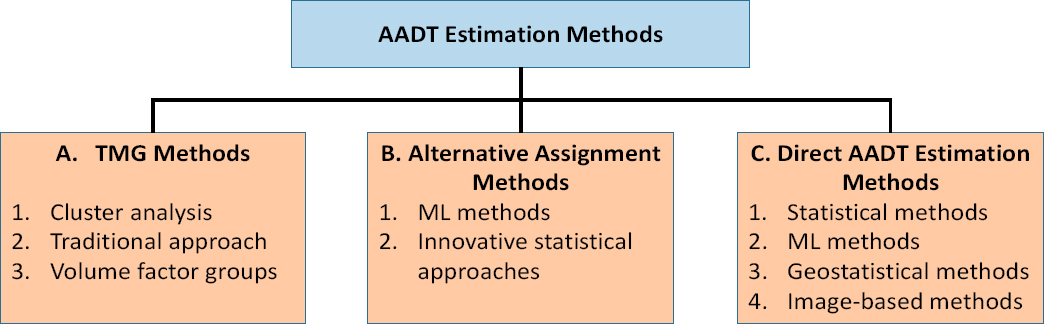
The three groups of methods are:
- Group A—TMG methods. The 2022 TMG describes three methods for creating factor groups (FHWA 2022):
- Cluster analysis.
- Traditional approach that requires local knowledge of the network.
- Volume factor groups.
- Group B—Alternative assignment methods. These methods are not described in the TMG and involve assigning SDCs to factor groups, particularly to clusters that may not be well-defined. The methods complement (as opposed to replace) cluster analysis and include:
- ML methods that are available in many statistical software programs.
- Other innovative data-driven approaches that employ statistical measures to determine similarities between an SDC and each factor group.
- Group C—Direct AADT estimation methods. These methods, also known as direct demand methods, directly estimate AADT from SDC, probe, and/or non-traffic data by avoiding the grouping and the assignment steps described above. The direct demand methods include statistical, ML, geostatistical, and image-based methods.
Each group of methods is presented below in a separate section.
Group A—TMG Methods
A brief description of each TMG method is provided Table 1. The main strengths and weaknesses of the three TMG methods are summarized in Table 2. All three TMG methods require traffic volume data from both CCSs and portable traffic recorders. The next three subsections provide more information about each method.
Table 1. Description of TMG Methods.
| Method | Description |
|---|---|
| Cluster Analysis | Cluster analysis, or clustering, is a classification method that aims to group the most similar CCSs together based on one or more common characteristics (e.g., 12 monthly adjustment factors) in order to minimize the within-cluster variability and maximize the between-cluster variability. |
| Traditional Approach | The traditional approach involves grouping CCSs based on general knowledge of the network and a review of monthly patterns. |
| Volume Factor Groups | This method involves creating traffic volume groups, with each group having a unique volume range. CCSs are assigned to the volume groups based on their AADT. |
Table 2. Main Strengths and Weaknesses of TMG Methods.
| Method | Strengths | Weaknesses |
|---|---|---|
| Cluster Analysis |
|
|
| Traditional Approach |
|
|
| Volume Factor Groups |
|
|
Cluster Analysis
Cluster analysis can be used to develop clusters or groups of CCSs that have similar traffic patterns. It uses statistical concepts for data exploration and analysis and employs algorithmic approaches for machine learning (ML) tasks (for more information about ML methods, see those described in Group B). The TMG recommends grouping CCSs based on their traffic patterns that are represented by the 12 MFs or the 84 MDWFs of each site (FHWA 2022). Overall, clustering produces more homogeneous factor groups (Schneider and Tsapakis 2009, FHWA 2022) and more accurate AADT estimates compared to the other two TMG methods (Krile et al. 2015).
Though there is a plethora of different types of clustering algorithms that have been used in various fields (Xu and Tian 2015), the most commonly used in the development of factor groups fall into two broad groups: (1) nonparametric methods that include agglomerative hierarchical clustering and partitioning clustering, and (2) parametric model-based clustering methods. The methods differ in (a) the types of data (e.g., quantitative or qualitative variables) that each algorithm is designed for, (b) whether similarities or dissimilarities between objects are calculated, (c) the metrics used to capture similarities or dissimilarities, and (c) how the objects are initially grouped. The nonparametric hierarchical methods initially assign each object to a group. At each step of the clustering process, the two most similar groups are merged into a new group. This process is repeated until all objects are grouped into a single cluster. The Euclidean distance is the most commonly used measure that quantifies the similarity between two objects.
In nonparametric partitioning clustering, users have to specify a priori the final number of clusters. The partitioning algorithm initially assigns each object to one of the predefined groups, and then at each step of the process, each object is moved to the most similar cluster based on a similarity measure/distance. The k-means method is the most popular partitioning algorithm. Because the optimal number of clusters is unknown, clustering is often performed multiple times—each time a different number of clusters is specified—and then the optimal number of clusters is selected based on one or more criteria, including engineering judgment, as explained later in this section. For example, Zhao et al. (2004) developed eight hierarchical clustering models using data from 129 sites in Florida. The authors used a statistic, called pseudo-F statistic, to determine the optimal number of clusters.
Where:
T = sum of squared Euclidean distances from each observation to the overall mean.
Pg = Euclidean distance measured from the observation in a given cluster to its cluster mean.
G = number of clusters at a given level of the hierarchy.
n = number of observations (i.e., sites).
The pseudo-F statistic was also used by Hasan and Oh (2020). Schneider and Tsapakis (2009) developed an innovative method for determining the optimal number of clusters by incorporating relevant American Association of State Highway and Transportation Officials (AASHTO) and FHWA recommendations (AASHTO 1992, FHWA 2001). The method was based on a weighted
coefficient of variation that was calculated every time cluster analysis was performed to develop a different number of clusters that ranged between 1 and n/5 clusters (n=total number of permanent sites) (Schneider and Tsapakis 2009).
Gecchele et al. (2011) and Rossi et al. (2014) developed hierarchical and partitioning models using CCS data from the Province of Venice, Italy. The authors determined the optimal number of clusters using the following criteria:
- Pseudo-F statistic.
- Analysis of the variance of the clusters.
- Davies-Bouldin Index.
- Practical considerations such as the need to have a reasonable number of CCSs per cluster.
The study found that all clustering methods resulted in seven optimal groups except for one partitioning method (X-means) that produced four clusters; however, the authors did not discuss nor provide the optimal number of clusters produced by each of the aforementioned criteria.
Regehr et al. (2015) applied cluster analysis and plotted the partial R-squared (R2) calculated for different number of clusters (1 through 1,152) obtained at each step of the clustering procedure (Figure 2).

Source: Regehr et al. (2015).
The optimal number of clusters was subjectively selected based on the rate of loss of homogeneity within the cluster analysis. The authors noted that the change in the semi-partial R2 was small until the number of clusters was eight (Regehr et al. 2015).
Sfyridis and Agnolucci (2020) applied the elbow method that involved calculating the total within-cluster sum of squares for different number of clusters and then selecting a critical point (five clusters in this study) beyond which the creation of more clusters resulted in a small decrease in the within-cluster variability (Sfyridis and Agnolucci 2020). Despite the usefulness of quantifying the within-cluster homogeneity and understanding how it varies with respect to the number of clusters, it is more important to know how the AADT accuracy changes as the number of clusters increases; this is one of the topics that this research investigates.
Many studies employed hierarchical clustering (Sharma and Allipuram 1993, Sharma and Leng 1994, Sharma et al. 2000) and partitioning clustering methods (Garber and Bayat-Mokhtari 1986, Flaherty 1993, Tsapakis 2009, Tsapakis et al. 2011a, Tsapakis et al. 2011b, Krile et al. 2015, Sfyridis and Agnolucci 2020) to develop factor groups. Most of the studies used the 12 monthly adjustment factors of CCSs as inputs to clustering. Wu and Zhang (2009) developed a co-clustering collaborative filtering method, which reduced the mean absolute percent error (MAPE) over the traditional approach by 33 percent. Tsapakis (2009) compared four traditional approaches against four enhanced cluster-based methods (Figure 3) using CCS data from Ohio. The author found that cluster analysis produced more homogeneous factor groups compared to the traditional approaches by up to 300 percent; however, the AADT accuracy of these methods was not determined.

Note: FC: Functional Classification, GC: Geographical Classification.
Source: Tsapakis (2009).
Figure 3 shows the average coefficient of variation of each method by year. The coefficient of variation was used to quantify the overall within-group variability associated with each method. Sfyridis and Agnolucci (2020) employed a K-prototype algorithm to cluster mixed type data from England and Wales that included over 40 independent variables. This algorithm integrated the k-means and k-modes algorithms that are suitable for numeric and categorical
variables, respectively. The variables were transformed using a min-max normalization to establish the same range (from 0 to 1) for all variables. The authors reported that transforming the data and performing clustering was key to improving the AADT accuracy. Krile et al. (2015) compared the three TMG methods (cluster analysis, traditional functional classification, and volume factor groups). Among several findings, the study concluded that clustering resulted in lower errors compared to the other two TMG methods; however, the study assumed that the group membership of the sample counts extracted from CCSs was known, which does not happen in practice with real SDCs.
Model-based clustering aims to determine the probabilistic density function for each cluster by estimating a vector of attributes. A maximum-likelihood criterion is used to merge groups (Zhao et al. 2004). Each cluster has three geometric characteristics: volume, shape, and orientation. These characteristics are used as independent parameters based on which various models can be built generating clusters with different characteristics. A three-letter code (E = equal, V = variable, I = identity) is used to represent the volume, shape, and orientation of the clusters created by a model. For example, the VEI model has variable volumes, equal shapes, and orientation on coordinate axes. Unlike the nonparametric clustering, model-based clustering can determine the optimal number of clusters by employing measures such as the Bayesian information criterion (BIC):
BIC = 2L − rlog(n)
Where:
L = log-likelihood of the model.
r = total number of parameters to be estimates in the model.
n = number of CCSs (Zhao et al. 2004).
Several studies have applied model-based clustering (Zhao et al. 2004, Li et al. 2006, Gecchele et al. 2011, Rossi et al. 2014). For example, Zhao et al. (2004) developed 10 parametric model-based clustering methods and found that incorporating both the 12 monthly adjustment factors and the geographic coordinates of the sites can assist in grouping sites that have similar patterns and are also located close to each other. The study also reported that functional class was not an important factor in developing factor groups and the latter were not stable over time. Gecchele et al. (2011) and Rossi et al. (2014) conducted a comparative analysis of hierarchical, partitioning, and model-based clustering methods and concluded that (a) no single method performed consistently better than the rest and the observed differences were attributed to a small number of sites, (b) all methods resulted in higher AADT accuracy than using a single factor group that contained all CCSs, and (c) model-based methods have a more robust mathematical structure compared to other clustering methods.
Advantages.
Cluster analysis is effective in identifying similar traffic patterns that may or may not be intuitively obvious (FHWA 2022). The clusters tend to be internally homogeneous because they are developed using a statistically valid and nationally accepted data-driven unbiased process, which uses similarity/dissimilarity measures. Therefore, the group adjustment factors are typically more precise than those produced from the traditional approach. The AADT estimates derived from annualized counts can also be more accurate than those produced by the traditional approach (Krile et al. 2015). In addition, clusters can be created efficiently using statistical programs.
Disadvantages.
The main disadvantage of cluster analysis is that the produced clusters may not have distinct characteristics that can be used to easily assign SDCs to factor groups. Because of this limitation, some clusters may be difficult to define and explain to others. Only a few studies have attempted to address this limitation. Regehr et al. (2015) developed a hybrid clustering approach by considering various assignment attributes including 24 hourly factors (HFs) calculated as ratios of hourly volumes to the average weekday volume. The authors stated that “roadway functional class, traffic volume, and land use characteristics are variables that can help explain the hourly traffic distributions evident from the cluster procedure—though a definitive causal link may not always be present” (Regehr et al. 2015). Hasan and Oh (2020) applied spatial k-nearest neighbors (KNN) clustering by incorporating four spatial and 11 temporal variables. The spatial variables included three binary variables (rural/urban, freeway, and arterial) and a continuous variable (population around a CCS). The temporal variables included four seasonal factors (winter, spring, summer, fall), three day-of-week factors (Monday through Thursday, weekend, and Friday), and four time-of-day adjustment factors (morning peak, morning off-peak, afternoon peak, and night off-peak). The optimal number of clusters (12) was estimated using the pseudo-F statistic. The results showed that the clusters from the proposed approach were more homogeneous (i.e., lower coefficients of variation) and produced on average more accurate AADT estimates than six clusters developed by the Michigan Department of Transportation.
Another major limitation of clustering is the lack of guidelines for determining the optimal number of clusters, particularly for nonparametric clustering methods. While mathematically this is feasible by employing optimization criteria (e.g., the BIC), the latter do not take into consideration practical limitations and guidelines. For example, with a few exceptions, the 2022 TMG recommends on average six CCSs per factor group (FHWA 2022); however, current optimization criteria may produce groups with a very small or very high number of CCSs. For instance, Zhao et al. (2004) used the BIC, which indicated that the optimal number of (model-based) clusters for 129 sites was two (2.0). Further, existing optimization criteria do not provide the flexibility to incorporate guidelines or other user preferences and constraints. As a result, engineering judgment is necessary to select a rational number of clusters and then make additional modifications, if needed. Another limitation is that the clusters tend to be unstable from one year to the next, complicating the development of factor groups (Faghri et al. 1996, Zhao et al. 2004). Also, cluster analysis may not be applicable to lower functional classes where only a few CCSs may exist in each state; the average number of CCSs on the three lowest roadway functional classes (rural minor collectors [6R], rural local roads [7R], and urban local roads [7U]) is 1.6 sites per state (Tsapakis et al. 2020a, Tsapakis et al. 2021a).
Traditional Approach
The traditional approach involves grouping sites based on general knowledge of the network and a review of monthly patterns. Roadway functional classification, rural/urban designation, and geographical stratification are commonly used approaches for developing an initial set of factor groups that analysts may need to refine further after reviewing the traffic patterns within each group. A typical modification of these groups includes identifying and moving recreational sites into one or more separate groups.
Many studies have examined the traditional approach (Drusch 1966, Hartgen and Lemmerman 1983, Erhunmwunsee 1991, Faghri et al. 1996, Stamatiadis and Allen 1997, Wright et al. 1997, Liu et al. 1998, Granato 1998, Sharma et al. 1999, McCord et al. 2003, Jiang et al.
2007, Jin and Fricker 2008, Jin et al. 2008, Schneider and Tsapakis 2009, Wu and Zhang 2009, Tsapakis et al. 2011a, Tsapakis et al. 2011b, Zhong et al. 2012, Desai et al. 2014, Figliozzi et al. 2014, Ha and Oh 2014, Tsapakis et al. 2014, Tsapakis and Schneider 2015, Krile et al. 2015, Islam 2016, Khan et al. 2018, Ahamed et al. 2019, Monney et al. 2020). In general, the most common attributes used in the traditional approach are the roadway functional class combined with the area type (i.e., rural/urban designation). Functional classification is often used alone in the case of lower volume roads that contain a small number of CCSs, as previously explained. Some states factor the counts taken on non–Federal aid system (NFAS) roads (i.e., functional classes 6R, 7R, 7U) using group adjustment factors from higher functional classes (Tsapakis et al. 2020a).
Many studies used the traditional approach as a baseline to quantify potential gains from other improved methods. For example, Drusch (1966) compared a traditional approach against another method that involved grouping CCSs based on similarities in their monthly adjustment factors over four consecutive years, as opposed to a single year, and then assigned seasonal counts to these groups. The author reported that the proposed method resulted in a smaller number of groups and required fewer seasonal counts per location, yielding significant cost savings over the traditional approach (Drusch 1966). Milligan et al. (2016) developed eight traditional factor groups and then assigned sample counts (extracted from permanent sites) to the closest permanent site within the same factor group. The study reported that the overall MAPE was 6.7 percent, but the errors marginally increased as the distance between an SDC and the expansion control site increased.
Advantages.
The main advantage of the traditional approach is the ability to create well-defined groups based on one or more characteristics that are readily available and easily accessible for a large portion of state transportation networks. These characteristics are also used to assign SDCs to one of the factor groups. The approach can be applied to all functional classes. In addition, it is simple and easy to understand and communicate to others (FHWA 2022). Because of these strengths, the approach has been widely used by many agencies for several decades.
Disadvantages.
The main disadvantage of the approach is that it tends to produce internally heterogeneous groups that may contain sites with highly variable patterns (Schneider and Tsapakis 2009). The group adjustment factors may not be representative of all different patterns within a group, potentially resulting in low accuracy of AADT estimates derived from SDCs (Tsapakis 2009). Further, the group adjustment factors may not meet the precision level (±10 percent) recommended by TMG at 95 percent confidence for nonrecreational roads (FHWA 2022). The approach relies on engineering judgment, which may be biased. Further, it may be challenging to maintain factor groups due to frequent changes made in the functional classification of some roads.
Volume Factor Groups
The volume factor group method involves creating a set of traffic volume groups, with each group having a specific AADT range. CCSs are assigned to the volume groups based on their AADT. The TMG recommends creating at a minimum five separate sets of volume factor groups: rural interstates, urban interstates, rural other roads, urban other roads, and recreational roads (FHWA 2022). Like the other traditional approaches, recreational sites need to be identified by reviewing seasonal and time-of-day patterns and then assign them to one or more recreational groups, if needed.
Though several agencies use volume factor groups, most previous research efforts focused on other traditional and nontraditional assignment methods. One of the studies that examined the performance of volume factor groups was conducted by Krile et al. in 2015. This is one of the most comprehensive studies in the literature that used CCS data from 32 states and compared the AADT accuracy and precision of the three TMG methods. The authors developed four volume factor groups using the following AADT ranges: AADT<1,000; 1,000≤AADT<10,000; 10,000≤AADT<100,000; and AADT≥100,000.
The results showed that the volume factor group method had the lowest performance compared to cluster analysis and the traditional functional classification approach (Krile et al. 2015); however, each method was developed using a different number of sites, making it difficult to conduct a direct comparison among methods. Further, the study considered only four volume groups, whereas in the case of the traditional approach, nine functional class groups were developed. That is, each volume factor group contained on average more sites than the functional class groups, potentially yielding more (internally) variable volume groups. In addition, the range of the third volume group (10,000≤AADT<100,000) was very wide, potentially contributing to the high variability of traffic patterns with this group. Additional research is needed to investigate the AADT accuracy and precision of more volume factor groups disaggregated into tighter volume ranges.
Advantages.
Similar to the traditional approach, the groups are well-defined based on one or more characteristics that are typically readily available at most agencies. Also, it is easy to explain the factor groups to others and assign counts to groups.
Disadvantages.
The main disadvantage of the approach is that it may produce heterogeneous groups that contain sites with different seasonal and time-of-day patterns. As a result, the group adjustment factors may not meet the precision level (±10 percent) recommended by TMG for nonrecreational roads (FHWA 2022). Likewise, the group adjustment factors may not be representative of all different roads within a group, potentially resulting in low accuracy of AADT estimates derived from annualized SDCs (FHWA 2022). The approach is subject to engineering judgment because analysts have to select the total number of volume factor groups and the volume range of each group. Further, the counts may be assigned to the wrong group because the true AADT at each SDC location is not known.
Group B—Alternative Assignment Methods
Several research studies have applied various methods that are not described in the TMG to assign SDCs to factor groups or individual CCSs. With a few exceptions, most of these studies focused on assigning counts to clusters, which were developed using some of the clustering methods described in the previous section. The alternative assignment methods include (a) known ML techniques that are available in many statistical software programs and languages, and (b) other innovative data-driven approaches that employ various statistical procedures and measures.
In general, statistics and ML have similarities in terms of methods, but their mechanisms are slightly different. Statistics rely on assumptions and draw population inferences from a sample. Any distortion from the assumptions can generate biased results. On the other hand, ML algorithms build a model based on training data to find generalizable patterns and then make predictions or decisions (Bzdok et al. 2018).
ML methods are traditionally divided into supervised and unsupervised learning methods. In supervised learning, users provide a training dataset that contains both inputs and their desired
outputs. The goal is to learn from the data and determine a function that can be used to predict the output associated with new inputs. Examples of supervised learning methods include neural networks, classification methods, decision trees, random forests, support vector machines, and others.
In unsupervised learning, users provide only inputs, so the goal of the algorithm is to find structure in the data (e.g., groups of objects). Examples of unsupervised learning methods include agglomerative hierarchical clustering, partitioning clustering, principal component analysis, and others. Other types of learning methods also exist, such as reinforcement learning; for more information, see Bishop (2006).
The subsections that follow describe various ML and innovative statistical assignment methods, respectively, that are available in the literature.
Machine Learning Methods
Several types of ML methods have been used in various fields for classification and prediction purposes. Table 3 briefly describes ML methods that have been used to estimate AADT, and Table 4 summarizes their main strengths and weaknesses (Murphy 2012, Shalev-Shwartz 2014).
Table 3. ML Methods Used to Assign SDCs to Factor Groups.
| Method | Description |
|---|---|
| Artificial neural networks (ANNs) | A collection of input, hidden, and output layers of interconnected neurons. Each neuron produces an output, which then becomes the input to the next layer. This continues until the terminal neurons produce an output. |
| Decision tree (DT) | A tree-shaped model that continuously splits the dataset into subsets based on one attribute at each split. The splitting process terminates when certain criteria are met. |
| Discriminant analysis (DA) | A model that finds linear combinations of common assignment characteristics between SDCs and factor groups and calculates the probability of group membership for each SDC. |
| Random forest (RF) | RF constructs multiple DTs from randomly selected subsets of the entire dataset. It can be used for classification and prediction. In the case of classification, the SDC is assigned to the CCS selected by most trees. In the case of prediction, the output is the average of all values predicted by the trees. |
| Gradient boosting (GB) | Unlike RF that builds several independent trees at once, GB starts by building a collection or ensemble of “weaker” trees and then iteratively and sequentially learns from each weak tree to build a stronger model. It can be used for prediction, classification, and ranking. |
| K-nearest neighbors | A method that can be used for classification and regression. It identifies the k most similar CCSs that are closer to an SDC. In the case of classification, the SDC is classified by a plurality vote of its neighboring CCSs and is assigned to its most similar CCS based on certain characteristics. The output is a class membership. In the case of regression, the output is a property value, which is the average of the values of the KNN. |
| Support vector machine (SVM) and support vector regression (SVR) | A method that uses a kernel function to transform non-linearly separated data from an input space to a feature space where data are linearly separated and then are transformed back to the input space, where they again become nonlinear. SVM is used for classification, and SVR is used for prediction. |
Table 4. Strengths and Weaknesses of ML Methods.
| Method | Strengths | Weaknesses |
|---|---|---|
| Artificial neural networks |
|
|
| Decision trees |
|
|
| Discriminant analysis |
|
|
| Gradient boosting |
|
|
| Method | Strengths | Weaknesses |
|---|---|---|
| K-nearest neighbors |
|
|
| Random forest |
|
|
| Support vector machines and support vector regression |
|
|
Among all these methods, four of them have been used to assign SDCs to factor groups: artificial neural networks, decision trees, discriminant analysis, and support vector machines. Table 5 summarizes previous studies that used ML methods in the assignment step. The other ML methods listed in Table 3 and Table 4 have been used for direct AADT estimation (Group C), as explained later in this chapter.
Table 5. Studies That Used Alternative Assignment ML Methods
| Author/Year | State/Year | Sample Size | Method | Attributes | Accuracy |
|---|---|---|---|---|---|
| Zhao et al. 2004 | FL 1997–2000 | 21 CCSs | Nonparametric and parametric clustering methods (grouping) and fuzzy decision tree (assignment) | 12 monthly adjustment factors and CCS coordinates for grouping & hotel visitors, ratio of seasonal households to permanent households, ratio of retail employment to retail employment, percentage of retired households with high income for assignment | Pool variance = 4.02–7.4 BIC = −4,149–40,194 |
| Li et al. 2006 | FL 2002 | 26 CCSs | Fuzzy decision tree | Hotel visitors, ratio of seasonal households to permanent households, ratio of retail employment to retail employment, percentage of retired households with high income | Information gain = 0.503 |
| Tsapakis et al. 2011a | OH 2005–2006 | 51 CCSs, 35,100 SDCs | Discriminant analysis | HFs, average daily traffic (ADT) | Mean absolute error (MAE) = 4.3–8.3 |
| Traditional approach | MAE = 12.1 | ||||
| Rossi et al. 2012 | Venice, Italy 2005 | 50 CCSs, 1,525 SDCs | Fuzzy C-mean (grouping) & ANN (assignment) | 84 MDWFs for grouping & HFs for assignment | MAPE = 9.5%–30.0% Standard dev. abs. percent error (SDAPE) = 7.5–46.6 |
| Gecchele et al. 2012 | Venice, Italy 2005 | 50 CCSs, 1,525 SDCs | Fuzzy C-mean (grouping) & ANN (assignment) | 84 MDWFs for grouping & HFs for assignment | MAPE = 4.2%–20.2% SDAPE = 4.0–22.3 |
| Tsapakis and Schneider 2015 | OH 2007–2008 | 49 CCSs, 24,900 SDCs | Discriminant analysis | ADT, HFs | MAPE = 5.50% SDAPE = 6.40 |
| Support vector machines | MAPE = 4.4% SDAPE = 5.2 | ||||
| Functional classification | MAPE = 13.1% SDAPE = 18.7 |
The studies listed in Table 5 are briefly described next, along with relevant considerations. Zhao et al. (2004) and Li et al. (2006) proposed a supervised fuzzy decision tree to assign SDCs to five seasonal factor groups, which were developed using model-based clustering. Prior to developing the DT, the authors performed regression analysis and found that the most influential factors for urban areas were the ratio of seasonal households to permanent households, hotel population or visitors, ratio of retail employment to retail employment plus population, and percentage of retired households with high income. The authors used these variables to develop a DT for urban roads. The tree calculated the probability of an SDC belonging to one of the factor groups; however, the study did not validate the performance of the tree and the accuracy of the AADT estimates derived from factored sample counts.
Tsapakis et al. (2011a) developed a series of DA models to assign counts to factor groups. DA is a supervised classification method that can be used to assign individual objects (i.e., SDCs) to groups of objects (i.e., factor groups) based on a set of common attributes. The principle of DA is the creation of discriminant functions that are linear combinations of a set of independent variables. The functions are used to classify objects into groups. A discriminant score was estimated for each discriminant functions as follows:
Dc = dc,0+ dc,1z1 + dc,2z2 + … + dc,pzp
Where:
Dc = standardized score of discriminant function c.
z = assignment variables that included 24 HFs and ADT.
p = number of assignment variables.
dc = discriminant function coefficient.
The study used several algorithms (the Wilks’ Lambda, Rao’s V, Mahalanobis distance, between-groups F, and the sum of unexplained variance) to systematically choose the most influential variables. The authors developed 12 DA models. Half of the models included both the ADT and the 24 HFs of each count, and the other models included only the 24 HFs. The results revealed that (a) the variable selection algorithm that produced the lowest MAPE (4.2 percent) is Rao’s V criterion followed by the Mahalanobis distance algorithm, (b) the 24 HFs were slightly more significant variables in the assignment process over the ADT, and (c) the DA models performed significantly better than a traditional functional classification approach that was used for comparison purposes.
Rossi et al. (2012) assigned counts to clusters using a multilayered, feed-forward, back-propagation neural network model. The HFs of each count were used as the assignment variables in the input layer of the neural network. The authors calculated the uncertainty associated with the assignment of a count to each factor group. The uncertainty was captured by two measures, non-specificity and discord. The AADT was estimated as a weighted average of SDC volumes adjusted by applying the adjustment factors of the assigned group(s), as follows:
AADT = w(1) × SPTC × fij1 + w(2) × SPTC × fij2
Where:
w(1), w(2) = weights calculated from the third step. The two weights capture the degree to which a count belongs to the first and the second group, respectively.
SPTC = daily volume of seasonal portable traffic count.
fij1 = adjustment factor for day-of-week i, month j, and group 1.
fij1 = adjustment factor for day-of-week i, month j, and group 2.
The proposed method resulted in MAPEs between 9.5 percent and 30 percent. The lowest errors were obtained for 72-hour sample counts (24- and 48-hour counts produced less accurate AADT estimates). Gecchele et al. (2012) applied the same method as that of Rossi et al. (2012) to estimate passenger car AADT using 2005 data from 50 CCSs in the Province of Venice, Italy. The reported MAPEs ranged between 4.2 percent (72-hour counts) to 20.2 percent (24-hour counts). The study concluded that discord and non-specificity were found to be useful measures of assignment uncertainty.
Tsapakis and Schneider (2015) compared three assignment methods: a traditional functional classification approach, discriminant analysis, and support vector machines. The SVM method uses a kernel function to transform data from an input space into a high-dimensional feature space F via a nonlinear mapping and then performs linear regression in this space. After a solution is found, it is transformed back to the input space, where it again becomes nonlinear. Four kernel functions were considered when developing the SVM models: linear, polynomial, Gaussian, and Laplace. The authors used two inputs to develop the DA and the SVM models: the ADT and the 24 HFs of each sample count extracted from 49 CCSs in Ohio.
The validation results showed that the Gaussian-based SVM model performed better than the other two methods by improving the MAPEs over the traditional approach by 65 percent. The study found that using both the ADT and HFs in SVM is more effective than using HFs alone. The opposite trend was observed in the case of DA. A possible reason is that the SVM transfers data from an input to a feature space, providing the ability to effectively assign counts using different types of data within the same SVM model. This is not feasible in discriminant analysis; however, the SVM methodology is more complicated than that of the DA. The next subsection describes previous studies that developed innovative statistical approaches.
Innovative Statistical Approaches
Table 6 lists studies that employed various statistical procedures and measures to assign counts to factor groups or individual CCSs.
Table 6. Studies That Used Innovative Statistical Approaches.
| Author/Year | State/Year | Sample Size | Method | Attributes | Accuracy |
|---|---|---|---|---|---|
| Sharma and Allipuram 1993 | WI | 24 CCSs | Index of assignment effectiveness (IAE) | SDC volumes from different months | Coefficient of variation of clusters = 0.13–0.38 |
| Davis and Guan 1996 | MN | 52 CCSs | Bayesian method | Daily counts | Estimation error = 5%–20% |
| Zhong et al. 2012 | Alberta, CA 2002–2009 | 357 CCSs | Coefficient of variation method using a Bayesian algorithm | Day of week, month of year | 95th percentile error = 13% |
| Traditional approach | 95th percentile error = 21.7% | ||||
| Lu et al. 2013 | FL 2000 | 116 CCSs | Assignment similarity score | Land use, roadway characteristics, demographic and socioeconomic variables | MAPE = 3.6%–4.2%, 75% of factors had error of 6% or less, 95% of factors had error of 10% or less |
| Tsapakis et al. 2014 | OH 2002–2006 | 250 CCSs, 142,177 SDCs | Discriminant analysis | Directional volumes | MAPE = 12.5%–14%, SDAPE = 14–15 |
| Weighted coefficient of variation | MAPE = 13%–15%, SDAPE = 14–15.5 | ||||
| Functional classification | MAPE = 16%–18%, SDAPE = 26–34 | ||||
| Milligan et al. 2016 | Manitoba, CA 5 years | 69 CCSs, around 2 million SDCs | Individual permanent counter expansion method | 24-hour and 48-hour counts, day of week, geographical information, proximity to urban centers, and dominant trip purpose | MAPE = 5%–10.5% |
The studies in Table 6 are briefly described next, along with their results and relevant considerations. Sharma and Allipuram (1993) proposed an assignment procedure that was based on an IAE, which measured the accuracy of assigning a count to a cluster. The assignment procedure included the following steps:
- Calculated mean squared errors (MSEs) as squared differences between the 12 MFs of every site and the corresponding 12 MFs of each group of permanent sites.
- Normalized the effectiveness of each assignment as follows:
Where:
AEi = effectiveness of each assignment for group i.
- Calculated the IAE as follows:
Where:
ni = number of times a sample site is assigned to group i.
AEi = the AE value for group i.
I = the total number of groups.
N = the total number of counts taken at a sample site during a year.
The authors proposed that establishing desired IAE target values (e.g., IAE > 95 percent and absolute percent error < 2 percent) might be beneficial in ensuring accurate assignments of counts to groups. The main limitation of this approach is that it requires multiple and long seasonal counts (e.g., seven-day counts) to be conducted within a year at the same site; however, this is not a common practice nowadays—many agencies prefer to take shorter and fewer counts at each site.
Davis and Guan (1996) developed a Bayesian method to assign an SDC to the factor group with the highest posterior probability, which was calculated as follows:
Where:
f(z1, … , zN|Gk) = a set of likelihood functions measuring the probability of obtaining the count sample if the site belonged to factor group Gk, for each k=1, …, n.
z1, … , zN = a sequence of N daily counts at an SDC site.
ak = prior classification probability that the given site belongs to Gk.
The prior classification probability was assumed to be 1/n (i.e., equal probability of a count belonging to any given factor group). A linear regression model was used as the likelihood function in the posterior classification probability. The model accounted for the month and day of week of each count. The validation results showed that the mean daily traffic estimation errors were around ±20 percent based on 14 sampling days selected from particular months and days of the week. In general, the method did not significantly improve the precision of the estimates compared to those obtained when adjustment factors are known. The method is complicated and time-consuming to develop and implement. It also requires long and frequent counts at each SDC site.
Zhong et al. (2012) introduced a novel pattern matching method, called the coefficient of variation ratio method. The authors first converted 48-hour counts to monthly ADT by using a growth factor and a day-of-month factor derived from a nearby site located on the same functional class. Then, the seasonal variation of the nearby CCS was compared to that of the SDC site using the coefficient of variation method as follows:
Where:
i = month of year (1, 2, …, 12).
MADT = monthly average daily traffic.
σ = standard deviation.
u = mean.
The CCS yielding the smallest coefficient of variation was selected as the best match, and its data were used to expand the SDCs. Furthermore, a Bayesian analysis was conducted to show the probability of each SDC belonging to each CCS. The results revealed that the coefficient of variation ratio method significantly improved the accuracy of AADT estimates (95th percentile error was around 12 percent) compared to the traditional roadway functional classification method, which produced a 95th percentile error of approximately 22 percent. A similar methodology and results were presented by Bagheri et al. (2015). This approach requires frequent SDCs (e.g., every month) to be taken at the same site throughout the year; however, this practice is not common in the United States.
Lu et al. (2013) identified influential factors that contribute to variations in monthly adjustment factors in rural areas in Florida and then developed and validated a method to assign factors to SDCs. The authors initially determined whether the hourly traffic patterns of sample SDCs extracted from 116 CCSs exhibited a single peak or a double peak. Then two sets of regression models were separately developed for single-peak and double-peak patterns, respectively. The 12 monthly adjustment factors of the permanent sites were used as dependent variables. The influential variables included a series of census and topological data. The authors used the influential variables as inputs to calculate an assignment similarity score that measured weighted normalized differences between two sites. The differences were weighted by the sum of partial R2 of each independent variable. The average MAPEs were between 3.6 percent and 4.2 percent. The results showed that 95 percent of the AADT estimates had an error of 10 percent or less, which is within the acceptable error range recommended by the Florida Department of Transportation (Lu et al. 2013). The proposed assignment method avoids the factor grouping process but requires a significant amount of census and other variables that may not be readily available and may be difficult and expensive to gather, process, and integrate into existing systems.
In 2014, Tsapakis et al. developed an assignment approach that involved calculating a weighted coefficient of variation (wCoV) between a count and each factor group. The wCoV was the weighted average of two coefficients of variation. The first coefficient of variation was calculated between the ADT of a count and the corresponding ADT of each factor group. The second coefficient of variation was calculated as the average coefficient of variation of every pair of time-of-day factors (those of the count and the corresponding factors of each group). The authors assigned different weights to each coefficient of variation to determine the optimal weights that produced the most accurate AADT. The results showed that (a) the 24 HFs were more important in the assignment process than the ADT, (b) the wCoV-based approach performed better than DA models, (c) the wCoV approach reduced the MAPE by approximately 8 percent over a traditional functional classification approach, and (d) DA improved the MAPE by 31 percent over the traditional method.
Milligan et al. (2016) aimed to determine the uncertainty associated with annualized AADT estimates from SDCs. The authors created eight factor groups based on geography, proximity to urban centers, and dominant trip purpose. Then, each sample SDC was annualized by applying appropriate adjustment factors from the closest permanent site within the same factor group. The method resulted in an overall MAPE of 6.7 percent. The study also found that the AADT estimation errors marginally increased as the distance between an SDC and the expansion control site increased.
The following general findings can be drawn about the alternative assignment methods in Group B in relation to the following key elements:
- Accuracy—Overall, the alternative methods produced more accurate results than the traditional approach. Many studies reported significant improvements in AADT accuracy over functional classification approaches. No study compared alternative assignment methods against volume factor groups. The alternative assignment methods complement cluster analysis; therefore, the two methods cannot be compared.
- Interpretability of factor groups—The majority of the alternative assignment methods assigned SDCs to factor groups, which were developed using clustering and/or engineering judgment. Therefore, the interpretability of the clusters was subject to the limitations associated with these two grouping methods (see previous section).
- Complexity—The alternative assignment methods are more complex than the traditional approach and the volume factor groups. With the exception of DTs, many ML methods are considered “black boxes,” and as such, their assignments cannot be easily interpreted. Most statistical approaches are more intuitive than the ML methods; however, they are not readily available in existing statistical software programs.
- Data requirements—The alternative assignment methods have higher data requirements than the TMG methods. Some alternative methods require (a) long and frequent counts to be taken at the same site throughout a year, though this is not a common practice nowadays; (b) census data to be downloaded, processed, analyzed, and integrated into existing data management systems; (c) time-of-day adjustment factors to be computed from CCS and SDC data, though they may not be currently available in existing systems; and (d) other topological variables (e.g., distance from SDC site to nearest CCS or major road) to be developed using GIS tools.
- Applicability to lower functional classes—The alternative assignment methods can be applied to both higher and lower functional classes. If the number of CCSs on NFAS roads is small and clusters cannot be developed, the alternative methods can potentially be used to assign SDCs to individual CCSs, as opposed to factor groups.
- Potential for integration into existing systems—ML methods that are available in statistical packages and languages could potentially be applied or integrated more easily into existing data management systems than innovative statistical approaches that need to be hard coded. The implementation cost will also be higher for methods that require many new data variables, as explained above.
Group C—Direct AADT Estimation Methods
These methods directly estimate AADT using various types of data by avoiding the grouping and assignment steps of the traditional approach. The methods can be broadly grouped
into four categories: statistical, ML, geostatistical, and image-based methods. Previous research studies that developed such methods used one or multiple data types that mainly include:
- CCS data—Permanent site data such as AADT and adjustment factors are mainly used as dependent variables to develop and calibrate AADT prediction models.
- SDC data—SDC data (e.g., ADT) may be used as the (a) dependent variable when there are limited or no CCS data available, particularly on lower functional classes; and (b) independent variables to train a model. In this document, the methods that use SDC data as independent variables are called count-based methods, whereas those that do not use SDCs as predictors are called non-count-based methods. This distinction is necessary because the data requirements and the anticipated accuracy of these two types of methods are considerably different.
- Probe data—Probe data include timestamped location data collected from phones, other mobile devices and tablets, global positioning system (GPS) devices embedded in vehicles, smartphone applications, and connected and autonomous vehicles. In this document, the methods that use probe data (including number of probe-based trips or trajectories) as independent variables are called probe-based methods, whereas those that do not use probe data as predictors are called non-probe-based methods. Likewise, this distinction is necessary because the data requirements and the anticipated accuracy of probe-based methods are different from those of non-probe-based methods.
- Non-traffic data—The non-traffic data include roadway (e.g., number of lanes), census (e.g., population and employment), topological (e.g., distance between a station and the nearest major road), temporal (e.g., day of week and month of year), vehicle (e.g., number of registered cars), and other types of data (e.g., satellite images, photos, weather data). The majority of the studies described in this section used non-traffic data either alone or in combination with some of the aforementioned data types. Some of the studies that used only non-traffic data produced disaggregated segment-specific AADT estimates, while others generated estimates aggregated by county, region, functional class, or other attributes (Shen et al. 1999, Seaver et al. 2000, Barrett et al. 2001, Zhao et al. 2004, Eom et al. 2006, Sun and Das 2015, Staats 2016, Morley and Gulliver 2016, Unnikrishnan et al. 2018, Chen et al. 2019). This project focused only on disaggregated segment-specific AADT estimates.
The next four subsections describe non-probe-based statistical, ML, geostatistical, and image-based methods, respectively. The last subsection presents studies that either used probe and other types of data to develop AADT estimates or evaluated probe-based AADT estimates developed by third-party data providers.
Statistical Methods
Regression is the most commonly used statistical method for directly predicting AADT. Regression quantifies the relationship between a dependent variable (i.e., AADT) and one or more independent variables. Regression is based on the following general assumptions (Chowdhury et al. 2019):
- A linear relationship exists between dependent and independent variables.
- The errors are normally distributed.
- The independent variables are not highly correlated.
- The variance of errors is similar across all independent variables.
In general, regression has been very well-documented in the literature (Chowdhury et al. 2019). Regression is intuitive and easy to implement, and the parameter coefficients are easy to interpret. If the relationship between the independent and dependent variables is linear, regression is often preferred over other, more complicated methods because of its simplicity. Regression is susceptible to overfitting, but it can be avoided using dimensionality reduction and regularization techniques. On the other hand, the parameter coefficients are estimated globally. Regression is not appropriate when the relationship between variables is nonlinear, and the predictors are not independent. It is sensitive to outliers and can also generate negative predictions (i.e., AADT values). For more information about linear regression, see Montgomery et al. (2012). Table 7 lists past studies that developed various regression models.
Table 7. Studies That Used Non-Probe-Based Statistical Methods to Directly Estimate AADT.
| Author/Year | Area/Period | Sample Size | Method | Attributes | Accuracy |
|---|---|---|---|---|---|
| Ritchie 1986 | WA 1980–1984 | Not reported | Regression | Vehicle classification | Not reported |
| Erhunmwunsee 1991 | WI | 24 CCSs | Multiple linear regression | SDCs | R2 = 0.99 |
| Simple linear regression | R2 = 0.95 | ||||
| Mohamad et al. 1998 | IN 1996 | Not reported | Regression | County demographic and socioeconomic variables | Mean squared prediction error = 0.051, R2 = 0.77 |
| Xia et al. 1999 | Broward County, FL 1997 | 450 SDCs | Regression | Roadway characteristics, functional classification, socioeconomic attributes, and accessibility | Percent difference = 1.31%–57% Avg. difference = 22.7%, R2 = 0.63 |
| Zhao and Chung 2001 | Broward County, FL 1998 | 816 SDCs | Regression | Functional classification, number of lanes, direct access to expressway, accessibility of a count station to regional employment, employment around a count station, population concentration in the service area of a road, and employment concentration in the service area of a road | R2 = 0.66–0.81 MSE = 50–80.17 Total error = −2.37–1.95 |
| Li et al. 2004 | FL 2000 | 27 CCSs | Regression | Demographic and socioeconomic data, roadway characteristics, and geographic location | Adjusted R2 = 0.20–0.90 |
| McCord et al. 2006 | OH | 12 CCSs | Regression | SDCs | Average absolute relative error = 0.025–0.090 |
| Author/Year | Area/Period | Sample Size | Method | Attributes | Accuracy |
|---|---|---|---|---|---|
| Simple average | Average absolute relative error = 0.03–0.095 | ||||
| Pan 2008 | FL | 6,000 SDCs | Regression | Roadway characteristics and socioeconomic attributes | MAPE = 32.0%–159.5% Adjusted R2 = 0.16–0.42 |
| Jin et al. 2008 | IN 2004 | 73 CCSs | Regression | SDCs, day of week, and month of year | MAPE = 8.8% SDAPE = 0.0814 |
| ANN | MAPE = 9.9% SDAPE = 0.0795 | ||||
| Fuzzy basis function network | MAPE = 9.9% SDAPE = 0.0817 | ||||
| Traditional approach (24 factors) | MAPE = 14.8% SDAPE = 0.0978 | ||||
| Traditional approach (60 factors) | MAPE = 9.3% SDAPE = 0.0836 | ||||
| Traditional approach (84 factors) | MAPE = 9.2% SDAPE = 0.0835 | ||||
| Yang et al. 2011 | Mecklenburg, SC 2007 | 243 road segments | Regression & smoothly clipped absolute deviation penalty (SCAD) | Satellite information, roadway characteristics, socioeconomic variables, and driving behavior | R2 = 0.659 90th percentile error = 2.50 |
| Regression | R2 = 0.50–0.659 90th percentile error = 2.74 | ||||
| Apronti et al. 2015 | WY 2012–2014 | 476 SDCs | Regression | Pavement type, access to | R2 = 0.64 Root mean squared error (RMSE) = 73.4 |
| Travel demand modeling | highways, predominant land use types, and | R2 = 0.74 RMSE = 50.3 | |||
| Logistic regression | population | 79%–88% of sites were correctly classified | |||
| Raja et al. 2018 | AL | 205 CCSs | Regression | Nearby population, number of households in the area, employment in the area, population-to-job ratio, and accessibility | Nash-Sutcliffe = 0.75 |
In general, most studies used different types of non-traffic data as independent variables. Socioeconomic, demographic, and roadway characteristics are the most frequently used data types. Many studies found that roadway variables such as number of lanes are more important
predictors than land use and sociodemographic variables (Xia et al. 1999, Zhao and Chung 2001, Eom et al. 2006, Pan 2008, Selby and Kockelman 2011, Lowry 2014, Keehan et al. 2017). Functional classification was used by Xia et al. (1999), Zhao and Chung (2001), Eom et al. (2006), Wang and Kockelman (2009), Lowry (2014), and Keehan et al. (2017). Roadway variables are typically more accessible within a transportation agency than land use and census variables (Unnikrishnan et al. 2018). Overall, non-count-based methods have lower predictive power compared to those that use SDC volume data as predictors. Although demographics, employment, and land use features affect AADT, the latter changes longitudinally, and their relationship cannot be simply described with a formula (Zhang et al. 2018).
Ritchie (1986) initially grouped CCSs by functional class, rural/urban designation, and region, and then performed regression analysis for each factor group and month of year. The AADT was used as the response and the 24-hour SDC volumes as independent variables. The volumes were estimated using 72-hour sample counts (Tuesday through Thursday) in each month. The regression coefficient was used as the adjustment factor for that month and factor group. The study did not report the accuracy of this method. One caveat of this approach is that it requires 72-hour counts, but nowadays many agencies conduct shorter counts on different days of the week.
Erhunmwunsee (1991) developed a multiple linear regression model to examine the effect of count duration on AADT accuracy. The author used SDCs conducted in different months at the same site as independent variables. The results showed that the longer the count duration, the better the AADT estimates, but the eight-hour count showed a fairly similar level of accuracy compared to longer counts. Including two SDCs from different months resulted in higher R2 than using simple linear regression.
Mohamad et al. (1998) developed the following non-count-based regression model for county roads in Indiana:
log10(AADT) = 4.82 + 0.82 ∗ location type + 0.84 ∗ easy access to highway + 0.24 ∗ county population − 0.46 x log10(total arterial mileage of a county)
The model resulted in R2 = 0.77. The authors validated the model using data from eight randomly selected counties that were not used in the model development process. The mean squared prediction error was 0.051, and the mean absolute percent error was 16.8 percent. The study also found that traffic volumes on local roads did not substantially vary within a day or a week. This finding suggests that factoring SDCs on these roads does not provide significant benefits, which is contradictory to previous findings by Stamatiadis and Allen (1997) and Wright et al. (1997).
Xia et al. (1999) also developed a non-count-based model to estimate AADT on non-state roads in Florida:
AADT = −10759 + 4737.44 ∗ number of lanes + 5071.13 ∗ functional class + 1274.17 ∗ area type + 0.15 ∗ automobile ownership − 816.21 ∗ accessibility to county roads − 0.15 ∗ service employment
The results showed that 85 percent of the test dataset resulted in errors lower than 40 percent. The final model explained 63 percent of the AADT variability.
Zhao and Chung (2001) developed four multiple linear regression models using several independent variables: functional classification, number of lanes, direct access to expressway, accessibility of a count station to regional employment, employment around a count station,
population concentration in the service area of a road, and employment concentration in the service area of a road. AADT was the dependent variable and was calculated as a simple average of AADT estimates derived from factored quarterly counts. The study found strong correlations between AADT and all eight independent variables. Functional classification and number of lanes were found to be the most significant variables. The R2 values of the models ranged from 0.66 to 0.82 and the mean square errors from 50.0 to 80.2.
Li et al. (2004) applied regression analysis to identify factors that affect seasonal variation in traffic. The authors used monthly adjustment factors as the dependent variable. The independent variables included roadway features, demographic and socioeconomic characteristics, and geographic spatial location dummy variables. The results showed that seasonal movements, retired people with high income, and retail employment were significant variables, indicating that seasonal factors are associated with fundamental causes that produce traffic rather than traffic information itself.
McCord et al. (2006) developed a linear regression model that included annualized coverage counts taken on multiple days. The AADT estimates were more accurate (average absolute relative error = 0.025–0.90) than those produced from the traditional approach (average absolute relative error = 0.030–0.095) where the coverage counts were simply averaged rather than being used in a regression model. One of the limitations of the methodology is that it requires long and frequent coverage counts that are not usually conducted in practice.
Pan (2008) developed six non-count-based linear regression models for state, county, and local roads in Florida using roadway, socioeconomic, and land use data. The results showed that the regression models resulted in MAPE values between 32 percent and 160 percent. The adjusted R2 values of the models varied from 0.166 to 0.418.
Jin et al. (2008) compared traditional 24-, 60-, and 84-factor approaches; an analysis of variance (ANOVA) model; ANN models; and fuzzy basis function network models. The ANOVA model included four independent variables: day-of-week effect, month-of-year effect, interaction term between day-of-week and month-of-year effects, and logarithm of the daily traffic volume from a count taken on a specific day of week and month. The logarithm of AADT was the dependent variable of the model. The authors applied these methods using 2004 data from nine permanent sites located on urban interstates in Indiana. Their findings showed that (a) the traditional 60- and 84-factor approaches had lower errors compared to the ANN, the fuzzy basis function network models, and the 24-factor approach; (b) ANOVA had the best performance among all methods; and (c) all the other approaches except for the traditional 24-factor approach produced MAPEs that were lower than 10 percent.
Yang et al. (2011) proposed a novel variable selection procedure that involved calculating SCAD. The procedure selected significant variables and estimated regression coefficients. Using 2007 traffic volume data from local roads in Mecklenburg County, North Carolina, the study developed three AADT estimation models: a SCAD-based model and two additional regression models developed by employing the backward and forward stepwise variable selection procedures. The non-count-based models included six variables: cars, lanes, housing units, income, below poverty line, and car intensity. Three of these variables (lanes, housing units, and income) were found to be important in all models, but they were not statistically significant when they were used alone in simple regression models. According to the results, the SCAD model resulted in an R2 of 0.659 and produced the lowest AADT estimation errors among all three models.
Apronti et al. (2015, 2016) developed non-count-based linear regression and logistic regression models to estimate ADT for low-volume roads in Wyoming. The linear regression model included four predictors: pavement type, access to highways, land use, and population by block group. The dependent variable was the log transformation of the ADT. The model resulted in an R2 of 0.64 and an RMSE of 73.4 percent. The correlation between the actual and the estimated log(ADT) values was 0.61. Logistic regression models were developed to predict the probability of each road segment belonging to one of five ADT thresholds: ADTs less than 50, 100, 150, 175, and 200. One model was developed for each threshold. The independent variables included land use, pavement type, total household, employment, employment density, per cap income density, house density, and population density. The logistic regression results showed that 79–88 percent of the road segments were correctly classified. In general, the study reported that the two regression models are recommended when quick estimates of traffic volumes are required, but not when a high level of AADT accuracy is needed.
Raja et al. (2018) developed non-count-based linear, quadratic, and logarithmic models to estimate AADT for low-volume roads in 12 counties in Alabama. The independent variables included nearby population, number of households in the area, employment in the area, population-to-job ratio, and accessibility. The linear and quadratic models performed similarly (Nash-Sutcliffe statistic = 0.75) and outperformed the logarithmic model (Nash-Sutcliffe statistic = 0.44).
Machine Learning Methods
Among all ML methods presented in Table 4 and Table 5 (Group B), three of them have been used in the past to directly estimate AADT: K-nearest neighbors, random forest, and support vector regression. Table 8 summarizes previous studies that used ML methods in the assignment step. These studies are also described after the table.
Table 8. Studies That Used Non-Probe-Based ML Methods to Directly Estimate AADT.
| Author/Year | State/Year | Sample Size | Method | Attributes | Accuracy |
|---|---|---|---|---|---|
| Sharma et al. 1999 | MN 1993 | 63 CCSs | ANN | 48-hour counts | 95th percent error (PE) = 14.1–16.7 MAPE = 6.9%–10.6% |
| Traditional approach | 95th PE = 15.3 MAPE = 4.4%–8.7% | ||||
| Sharma et al. 2000 | Alberta, Canada | 55 CCSs | ANN | 48-hour counts | 95th PE = 21.8–63.6 MAPE = 8.9%–16.6% |
| Unfactored sample average | 95th PE = 47.6–103.1 MAPE = 10.6%–14.1% | ||||
| Sharma et al. 2001 | Alberta, Canada 1996 | 55 CCSs | ANN | 48-hour counts | 95th PE = 21.8–37.7 MAPE = 8.9%–21.7% |
| Unfactored sample average | 95th PE = 27.6–40.1 MAPE = 19.9%–27.8% | ||||
| IN 2004 | 56 CCSs | KNN | Geographical spatial location index, roadway | MAPE = 7.3% SDAPE = 0.0865 |
| Author/Year | State/Year | Sample Size | Method | Attributes | Accuracy |
|---|---|---|---|---|---|
| Jin and Fricker 2008 | Traditional approach (24 factors) | characteristics, land use attributes, socioeconomic data | MAPE = 11.4% SDAPE = 0.1025 | ||
| Traditional approach (84 factors) | MAPE = 7.8% SDAPE = 0.0906 | ||||
| Castro-Neto et al. 2009 | TN 1985–2004 | 11,000 SDCs | SVR | 24-hour and 48-hour counts | MAPE = 2.1%–2.3% RMSE = 0.0141–0.0344 |
| Regression | MAPE = 3.7%–3.9% RMSE = 0.021–0.056 | ||||
| Holt exponential smoothing | MAPE = 2.6%–2.7% RMSE = 0.018–0.050 | ||||
| Islam 2016 | SC 2011 | 117 CCSs | ANN | Hourly traffic volumes, roadway attributes and socioeconomic characteristics including income, employment, percent of population below poverty, number of vehicles, number of housing units, day of week, month of year, and number of lanes | RMSE (Urban Arterial) = 0.3–1.1 |
| SVR | RMSE (Urban Arterial) = 0.2–0.6 R2 = 0.84 MAPE = 6.8%–16.3% | ||||
| Regression | MAPE = 45.3% | ||||
| Traditional approach | R2 = 0.80 MAPE = 21.22% | ||||
| Khan et al. 2018 | SC 2016 | 112 CCSs | ANN | Socioeconomic information, functional classification, day of week, month of year | RMSE = 0.31 MAPE = 14.8% |
| SVR | RMSE = 0.33 MAPE = 13.6% | ||||
| Regression | MAPE = 23.5% | ||||
| Traditional approach | MAPE = 16.4% | ||||
| Nasri et al. 2019 | MD & NM 2015 | ANN | Demographics, socioeconomic, and built environment characteristics, raw GPS data | MSE = 0.019 (MD) MSE = 0.008 (NM) RMSE = 0.14 (MD) RMSE = 0.086 (MN) R2 = 0.71 (MD) R2 = 0.95 (MN) | |
| Spatial autoregressive model | MSE = 0.026 (MD) MSE = 0.014 (NM) RMSE = 0.16 (MD) RMSE = 0.12 (MN) R2 = 0.63 (MD) R2 = 0.93 (MN) | ||||
| Regression | R2 = 0.50 (MD) R2 = 0.87 (MN) |
| Author/Year | State/Year | Sample Size | Method | Attributes | Accuracy |
|---|---|---|---|---|---|
| GPS method | Not reported | ||||
| Chowdhury et al. 2019 | SC 2011–2016 | 112 CCSs | SVM | Socioeconomic data, roadway characteristics | RMSE = 0.22–0.46 MAPE = 11.3%–19.8% |
| ANN | RMSE = 0.25–2.15 MAPE = 11.9%–124.4% | ||||
| Regression | R2 = 0.74 MAPE = 15.1%–31.9% | ||||
| Origin-destination centrality model | Not reported | ||||
| Tawfeek and El-Basyouny 2019 | Alberta, Canada | 1,350 four-legged intersections | ANN | Road geometry, network and accessibility | R2 = 0.89 |
| Regression | R2 = 0.66 | ||||
| Sfyridis and Agnolucci 2020 | England & Wales 2016 | 19,000 SDCs | SVR | Vehicle type, socioeconomic, land use, roadway features, accessibility | Weighted MAPE = 14.5% RMSE = 2,336 |
| RF | Weighted MAPE = 14.5% RMSE = 2,119 | ||||
| Regression | Weighted MAPE = 15.7% RMSE = 2,413 | ||||
| Das and Tsapakis 2020 | Vermont | 2,369 SDCs | SVR | Population density, work area characteristics, demographic, socioeconomic, geometric characteristics | RMSE = 423–1,066 R2 = 0.09–0.24 |
| RF | RMSE = 396–992 R2 = 0.19–0.36 | ||||
| KNN | RMSE = 410–1,066 R2 = 0.09–0.26 | ||||
| Regression | RMSE = 448–1,064 R2 = 0.08–0.27 | ||||
| Generalized linear model | RMSE = 423–1,066 R2 = 0.08–0.27 |
Sharma et al. (1999) developed multilayered feed-forward back-propagation ANN models using data from 63 CCSs in Minnesota. One model (ANN1) was developed for all study sites without considering the day or month of counting, and a second set of models (ANN2) was separately constructed for each group of sites by accounting for day-of-week and monthly variation in traffic. Forty-eight hourly adjustment factors from sample counts were used as inputs to train the models. The number of neurons in the hidden layer was equal to half of that in the input layer (24=48/2). There was one neuron in the output layer of each model. The 95th percentile errors for ANN1, ANN2, and a traditional method were approximately 23 percent, 20 percent, and 15 percent, respectively. A likely reason behind the high errors of the ANN models was that the permanent sites were grouped using only 21 (day-of-week monthly) adjustment factors for the counting period April through October—not 48-hour volume patterns. In other words, the sites within a group can have similar day-of-week monthly factors but different hourly volume patterns over any 48-hour period.
Similar to the 1999 study, Sharma et al. (2000) developed and compared neural networks against three traditional AADT estimation approaches by focusing on low-volume roads (AADT<1000 vehicles per day [vpd]) in Alberta, Canada. The three traditional approaches resulted in (a) a single group of all 55 study sites, (b) four groups (agriculture/resource, resource, tourist/resource, and tourist), and (c) five groups that were based on a hierarchical grouping approach. ANN models were separately developed using one and two 48-hour counts taken at different times. The results showed that the hierarchical grouping approach produced the lowest MAPE (10.6 percent) among the three traditional methods. It also performed better than the ANN, which considered a single 48-hour count in a year; however, the ANN models with two 48-hour counts outperformed all methods. The authors also concluded that dividing low-volume roads (0–1,000 vpd) into smaller volume groups (e.g., 0–500, 501–750, and 751–1,000 vpd) did not have any impact on the results.
In 2001, Sharma et al. developed ANN models to predict AADT on low-volume roads in Alberta, Canada. The authors divided 55 CCSs into three volume groups (AADT≤500, 500<AADT≤750, and 750<AADT≤1000) and created one ANN model for each group. The study concluded that a single 48-hour count resulted in the highest average 95th percentile error. However, conducting two 48-hour counts within a year can reduce the 95th percentile errors to about 25 percent in most cases. The results of a similar analysis using three 48-hour counts indicated that the accuracy of AADT estimates did not improve significantly.
Jin and Fricker (2008) developed KNN models using the following inputs: geographical spatial location index (i.e., northwest, northeast, central, metropolitan, southwest, and southeast), functional classification, number of lanes, posted speed limit, and population and employment density within a 10-mile buffer around each site. The authors used 2004 data from 55 permanent sites in Indiana to develop 12 models: 24-hour traditional factor approach, 84-hour traditional factor approach, five unweighted KNN models that were based on different values of k ranging from 5 to 9, and the corresponding five KNN models that were weighted based on the distance between a count and a site. The results revealed that the traditional 24-hour factor approach resulted in the highest errors in most cases. The unweighted KNN with k = 9 produced the lowest errors.
Castro-Neto et al. (2009) developed an SVR model with data-dependent parameters using traffic counts from 25 counties in Tennessee. Two other models, namely Holt’s exponential smoothing and ordinary least square (OLS) regression model, were also developed for comparison purposes. The results revealed that the proposed SVR model performed better in the case of urban and rural roadways (MAPE = 2.3 percent, RMSE = 0.0344).
Islam (2016) compared the traditional factor approach against count-based SVR, ANN, and OLS models developed from sample counts generated from 117 CCSs in South Carolina. The training dataset contained hourly traffic volumes, roadway, socioeconomic, and other characteristics such as number of registered vehicles, day of week, and month of year. The authors employed a sequential feature selection procedure to select the most significant variables. Various models were developed separately for each functional class. Daily adjustment factors were used as the dependent variable in all models. The study concluded that the SVR model outperformed the other approaches for the majority of roadway functional classes.
Similar to the four methods presented by Islam (2016), Khan et al. (2018) conducted a comparative analysis of two ML methods (ANN and SVM), an OLS regression model, and a traditional functional classification approach. Hourly factors, socioeconomic data, and temporal information were used as independent variables. The authors considered nine different subsets of
these variables to construct various models. Similar to the conclusions drawn by Islam (2016), the authors found that the SVM model outperformed the other methods. Among all SVM models, the one that included hourly factors, day of week, and month of year resulted in the lowest prediction errors.
Zhang et al. (2018) and Nasri et al. (2019) aimed to improve the accuracy of vehicle miles traveled estimates for NFAS roads by applying several OLS regression, ANN, and spatial autoregressive models. Separate models were built for Maryland and New Mexico. The independent variables included the number of through lanes, population, number of workers earning $3,333/month or more at home, number of workers earning $3,333/month or more at work, jobs within 45 minutes from home, retail jobs within a five-tier employment classification scheme, median household income, entropy of employment, AADT of nearest local road or minor collector, and AADT of nearest major collector. The results of all models in both states showed that the ANN model performed better than the SAM and the OLS models in terms of R2 (0.71–0.95), MSE (0.019–0.008), and RMSE (0.14–0.086).
Chowdhury et al. (2019) compared various SVM, ANN, origin-destination (OD) centrality, and OLS regression models. The 365 daily adjustment factors were used as the dependent variable. The most significant variables were determined by employing a sequential feature selection procedure. Different models were separately developed for various functional classes. The authors used nine different subsets of independent variables to identify the most effective combination of predictors. The most effective SVM model included temporal categorical variables and 24 HFs (i.e., it did not include socioeconomic features). The SVM model outperformed all other models for all roadway functional classes.
Tawfeek and El-Basyouny (2019) applied a count-based neural network to estimate AADT for minor roads at 1,350 rural four-legged stop-controlled intersections in Alberta, Canada. The dataset used in this study contained traffic volumes for both major and minor roads, geometric characteristics (e.g., right/left turn lanes on major road, number of lanes, presence of median, etc.), and network characteristics (e.g., service class, closeness to urban centers, type of the closest urban center). The authors concluded that the neural network model improved the R2 by 35 percent over a linear regression model that was developed for comparison purposes.
Sfyridis and Agnolucci (2020) first created clusters of different types of roads in England and Wales and then developed SVR, RF, and linear regression models for each cluster separately. The results showed that SVM had the best overall performance (weighted MAPE = 14.47 percent) followed by the RFs (weighted MAPE = 14.48 percent). The study concluded that the small sample size in some clusters affected the performance of the regression models.
Das and Tsapakis (2020) developed three types of non-count-based ML models (RF, SVM, and KNN) and two statistical models (linear regression and generalized linear models) to estimate AADT for uncounted low-volume roads in Vermont. Models were separately developed for the three lowest functional classes, rural minor collectors, and both rural and urban local roads. The training dataset included roadway, demographic, socioeconomic, and work area characteristics. Among all models, the RF models yielded the highest R2 and lowest RMSEs for all functional classes. Population density and work area characteristics were the most influential predictors.
Geostatistical Methods
Geostatistical methods use data at certain locations where a specific variable (e.g., traffic volume counts) is measured to predict values at uncounted locations. Geostatistical approaches
are based on spatial interpolation. The basis of these methods is that some variables are autocorrelated over space and the level of autocorrelation decreases with distance. Geographical weighted regression (GWR), kriging, and incorporation of topological variables in statistical models are the most commonly used geostatistical methods. Table 9 provides a brief description of each method, and Table 10 summarizes their main strengths and weaknesses.
Table 9. Geostatistical Methods Used to Directly Estimate AADT.
| Method | Description |
|---|---|
| Geographical weighted regression | A spatial interpolation method that allows model parameters to be estimated in space locally, as opposed to globally. GWR allows different relationships to exist between the dependent and independent variables at different locations. |
| Kriging | Predicts the value of a variable at a specific location by using other known values in the vicinity of that location. Kriging uses the spatial correlation between sampled points to interpolate the values in space. It generates estimates of the uncertainty surrounding each interpolated value. Variogram is an important input in kriging interpolation. It is a measure of spatial correlation between two points. |
| Topological variables in statistical models | Involves developing and incorporating topological variables in statistical models such as regression. The topological variables aim to determine the relative importance or cost of specific roadway network elements such as links. The importance can be captured by how many times a link is used by roadway users. |
Table 10. Strengths and Weaknesses of Geostatistical Methods.
| Method | Strengths | Weaknesses |
|---|---|---|
| Geographical weighted regression |
|
|
| Kriging |
|
|
| Topological variables in statistical models |
|
|
Table 11 provides a summary of studies that used geostatistical methods. The methods and the studies are described after the table.
Table 11. Studies That Used Non-Probe-Based Geostatistical Methods to Directly Estimate AADT.
| Author/Year | State/Year | Sample Size | Method | Attributes | Accuracy |
|---|---|---|---|---|---|
| Zhao and Park 2004 | FL 1998 | 775 SDCs | GWR (bi-square weighting) | Number of lanes, accessibility, population, employment, and direct access to expressways | MSE = 35.6 Akaike Information Criterion (AIC) = 5,160 R2 = 0.87 |
| GWR (Gaussian weighting) | MSE = 37 AIC = 5,181 R2 = 0.87 | ||||
| Regression | MSE = 55.8 AIC = 5,323 R2 = 0.76 | ||||
| Wang and Kockelman 2009 | TX 1999–2005 | 200 CCSs | Kriging | Functional class | Median error = 0.31 |
| Selby and Kockelman 2011 | TX 2005 | 28,000 SDCs | Universal kriging | Roadway characteristics, socioeconomic variables | MAPE = 16%–79% |
| Lowry and Dixon 2012 | ID 2005 | Regression | Connectivity importance index, betweenness | Not reported | |
| Lowry 2014 | ID 2005 | 341 road segments | Regression | Notion of centrality (e.g., internal-external, OD centrality) | Median APE (MdAPE) = 22% R2 = 0.95 |
| Morley and Gulliver 2016 | UK 2013 | 4,462 SDCs | Poisson generalized linear model (route-based) | Known minor road AADT, road class, urban/rural location, nearest major road AADT, index of connectivity | R2 = 0.62 RMSE = 4.36 |
| Fixed AADT | R2 = 0.38 RMSE = 5.6 | ||||
| Fixed AADT (classified) | R2 = 0.59 RMSE = 4.6 | ||||
| Keehan et al. 2017 | Greenville, SC 2015 | 6 CCSs, 109 SDCs | Regression (centrality-based) | Roadway characteristics, functional class, link significance index | R2 = 0.66 RMSE = 7,352 |
| Travel demand model | R2 = 0.61 RMSE = 14,073 |
Unlike regression that estimates model parameters globally, GWR estimates model parameters locally. GWR allows different relationships to exist between the dependent and independent variables at different locations. Zhao and Park (2004) developed GWR models using factored SDCs collected in Broward County, Florida, as the dependent variable. Five independent variables were used in the models: number of lanes, accessibility, population, employment, and direct access to expressways. The GWR models performed better than an ordinary linear regression model that was developed for comparison purposes. The R2 values of the linear regression model and the best performing GWR model were 0.764 and 0.876,
respectively. In general, GWR can more effectively capture the relationship between AADT and the independent variables spatially, which cannot be captured in linear regression.
Another geostatistical method is kriging. The goal of kriging is to predict the value of a variable at a specific location by using other known values in the vicinity of that location. The target variable is predicted as follows:
Zi(s) = μi(s) + εi(s)
Where:
Zi(s) = target variable (i.e., traffic volume) at location s of site i.
μi(s) = deterministic trend estimate.
εi(s) = random errors that are spatially correlated.
There are three main types of kriging: (a) ordinary kriging, where μ(s) is constant; (b) universal kriging, where μ(s) depends on other independent variables; and (c) simple kriging, where μ(s) is known. Wang and Kockelman (2009) developed an ordinary kriging model for uncounted segments in Texas. The Euclidean distance was used to spatially interpolate AADT values at roadway locations that belonged to the same functional class. The results showed that (a) traffic volumes in different functional classes exhibited different patterns of spatial autocorrelation, (b) GWR outperformed the methods that are based on spatial extrapolation (i.e., assigning AADT values from the nearest sampling site), and (c) the performance of the GWR model was significantly better when estimating AADT for segments with traffic volume higher than 1,000 vpd.
Selby and Kockelman (2011) applied universal kriging to predict AADT for uncounted segments in Texas. Box-Cox transformed traffic counts were used as the response variable. A structured error term was defined as a function of the distance between two locations calculated using (a) the shortest-path network distance and (b) the Euclidean distance. The authors developed non-count-based kriging models using roadway characteristics (e.g., number of lanes, speed limit, and functional class) and population and employment density variables as predictors. Universal kriging provided more accurate (16–79 percent reduction in mean absolute error) and reliable results (48 percent increase in adjusted R2) than non-spatial regression models. The authors also found that network-based kriging models did not offer any improvement over those that used the Euclidean distance.
In addition to GWR and kriging, some studies incorporated topological centrality variables in statistical models to determine the importance of specific roadway network elements such as links. For example, Lowry and Dixon (2012) developed five GIS-based tools to process data and estimate AADT. The authors calculated a connectivity importance index for every street in the network. The index was used as an independent variable in linear regression models; however, the accuracy of the models was not reported.
In 2014, Lowry developed an OLS count-based model that included a network analysis metric, called stress centrality, which quantified the topological importance of a link in a network. The metric was calculated as follows:
Where:
V = the set of all nodes in a network.
σi,j = the shortest path from node i to node j. σi,j
σi,j(e)
Stress centrality captures the number of times a link would be used if someone travels from every node to every other node in the network via the shortest path. The R2 values of the model were close to 1.0, and the MAPE was 22 percent. However, the method is suited for small and medium-sized networks. Gathering data for all roads within a state’s network would require extensive time and resources.
Morley and Gulliver (2016) compared three methods to estimate AADT for minor roads in the UK: (1) a fixed approach that assumed a constant flow of 500 vpd on all minor roads; (2) a classified approach that assigned the national median AADT on four types of minor roads (residential, unclassified, tertiary, secondary) that were further divided by rural and urban area; and (3) a Poisson generalized linear model that used a route importance indicator, which was calculated by assigning a cost to each segment. The assigned cost values were input to a Dijkstra routing algorithm to determine how many times a minor road was traversed. The general form of the generalized linear model was:
AADT = log(Route Importance) + (OSM Road Type) + log(AADT on nearest major road) + Urban or Rural
The routing method was found to moderately underpredict the observed AADT for both major and minor roads. The validation results showed that the routing approach (R2 = 0.62) outperformed the fixed approach (R2 = 0.38) and the classified approach (R2 = 0.59).
Keehan et al. (2017) used stress centrality and OD centrality variables along with the roadway functional class, number of lanes, and speed limit to develop multiple linear regression models. The OD centrality measure was calculated as follows:
Where:
N = the number of lanes on link e.
V = the set of all nodes in a network.
σi,j = the shortest path from node i to node j.
σi,j(e)
Wi = the relative weight of origin i.
Wj = the relative weight of destination j.
The results showed that the centrality-based model outperformed an existing traditional travel demand model used by the City of Greenville in terms of R2 (0.77 vs. 0.61) and RMSE (7,352 vs. 14,073).
Image-Based Methods
Some studies estimated AADT using satellite images, air photos, and other data (Table 12). For example, McCord et al. (2003) estimated AADT using satellite imagery and air photos of interstate highway segments equipped with CCSs. Their approach included the following steps: (1) determine vehicle density from each image, (2) convert the density to an SDC volume, (3) expand the SDC volume to an hourly volume, (4) expand the hourly volume to a daily volume, and (5) annualize the daily volume. The results showed that the relative AADT estimation errors ranged between −29 percent and 31 percent.
Table 12. Studies That Used Non-Probe Image-Based Methods to Directly Estimate AADT.
| Author/Year | State/Year | Sample Size | Method | Attributes | Accuracy |
|---|---|---|---|---|---|
| McCord et al. 2003 | OH | 14 satellite images | Adjusted traditional approach (using image data) | Satellite imagery and air photos | Relative error = −29%–31%, Mean error = 0.02 |
| Traditional approach | |||||
| Goel et al. 2006 | OH | 386 road segments | Bayesian approach (using imagery data and coverage counts) | Imagery data, ground counts | Relative error = 0.70%–0.90% |
| Jiang et al. 2007 | OH 2005 | 5 CCSs | Traditional approach (using air photos and coverage counts) | Space mean speed and air photos | Mean absolute relative error = 0.04 |
| Traditional approach (using coverage counts) | Mean absolute relative error = 0.05 | ||||
| McCord and Goel 2011 | OH 2003–2004 | 12 satellite images | Traditional approach (using air photos and coverage counts) | Satellite imagery and air photos | Mean absolute relative error = 0.24–0.14 |
Goel et al. (2006) developed a Bayesian framework to estimate statewide annual average OD flows using link-level AADT estimates from imagery and satellite data as well as ground-based counts. The Bayesian inferences considered different sources of uncertainty in the data. An estimate of OD flows was also calculated using portable traffic recorders and was compared against the estimates produced by the images. The results showed that the estimates calculated from six independent images of the same link produced similar estimates to those calculated from two-day counts. The authors concluded that having at least two images for each segment could reduce the estimation errors as well as the number of SDCs taken in the field.
Jiang et al. (2007) also used 12 images for six CCS-equipped locations. A dataset containing SDCs, air photos, and segment length was used to empirically apply and validate the proposed method, which included the following steps: (1) divide the number of vehicles shown in an image by the length of the corresponding segment to determine vehicle density; (2) multiply the density by the estimated space mean speed of the segment to estimate an hourly volume; (3) convert the hourly volume to an estimated daily volume by multiplying by 24 (hours) and an hourly factor that captures the temporal variation of the flow in a given hour of a specific day; and (4) adjust the daily volume by a day-of-week and monthly adjustment factor. The results showed that incorporating image-based information (image and coverage-based estimates) decreased the average estimation errors compared to the AADT estimates derived from coverage counts. The method requires a significant number of aerial images and manually counting the vehicles shown in the images. These activities can be time-consuming and
expensive. In addition, the method was applied using data from only six sites; a larger sample size is needed to examine the validity of the method under different traffic and weather conditions.
As a continuation of a previous research effort (McCord and Goel 2009), McCord and Goel (2011) conducted additional empirical studies using 12 images of highway segments where CCSs were located. The authors calculated the standard deviation of the ratio of an AADT estimate derived from images to an AADT calculated from CCS data. The study found that the estimates of the standard deviation parameter were more accurate that those produced when the default value of this parameter was used. The mean absolute relative errors were between 0.0283 and 0.1359; however, the method was not compared against other AADT estimation methods, making it difficult to understand its effectiveness. The report did not state the level of effort and costs required to fully implement this method statewide.
Probe-Based Methods
Probe data obtained from cell phones and GPS devices can characterize and quantify traffic volumes along a segment, provided that a sufficient number of probe devices passed along that segment. The ability to scale to the entire network without having to conduct a high number of SDCs creates a value proposition, which departments of transportation (DOTs) have started to explore (Pack and Ivanov 2021). Big data analytics’ capabilities are growing but are mainly supported by the private sector. Transportation agencies are interested in developing a better understanding of the capabilities and limitations associated with the use of probe data in AADT estimation.
The next two subsections present studies that (a) used probe, CCS, and other types of data to develop AADT estimates; and (b) evaluated probe-based AADT estimates developed by third-party data providers. The term “probe-based AADT estimates,” or simply “probe AADT estimates,” refers to AADT values estimated using a combination of different data types (e.g., CCS, SDC, probe, and/or other non-traffic data)—not just probe data.
Development of Probe AADT Estimates. Considering the recent introduction and use of probe data in traffic monitoring applications, only a few studies (Table 13) have presented probe-based AADT estimation methods that include statistical, ML, and geostatistical methods.
Table 13. Studies That Developed Probe-Based AADT Estimates.
| Author/Year | State/Year | Sample Size | Method | Attributes | Accuracy |
|---|---|---|---|---|---|
| Chang and Cheon 2019 | Ulsan City, S. Korea | K survey sites weighted power curve | AADT, annual average daily probe (AADP) traffic, functional class | MAPE = 7.2% | |
| Regression | MAPE = 9.5% | ||||
| Geographically weighted regression | MAPE = 10.6% | ||||
| Kriging | MAPE = 42.2% | ||||
| Iio et al. 2019 | TX 2017, 2019 | 949 short count stations | Cardinality | Probe point data from different road functional classifications and different volume level | Mean abs. differ. (MAD) = 3,261 Mean signed differ. (MSD) = 1,186 MAPE = 57.1% RMSE = 2,095 |
| Zhang and Chen 2020 | KY 2015–2017 | 13,575 SDCs | RF | Functional classification, area type, number of lanes, and probe vehicle data | R2 = 0.91 MAPE = 36.0% MdAPE = 25.8% Median Absolute Error (MdAE) = 411.75 MAE = 1293.75 |
| Regression | R2 = 0.88 MAPE = 41.0% MdAPE = 30.0% MdAE = 431.9 MAE = 2019.5 | ||||
| ANN | R2 = 0.90 MAPE = 37.5% MdAPE = 28.1% MdAE = 440.0 MAE = 1530.3 | ||||
| FHWA 2021 | 48 states 2019 | 4,255 CCSs | Regression | CCS, probe, and other non-traffic data that were not specified | MAPE = 36.3% Normalized RMSE = 24.05 |
| Elastic net regression | MAPE = 23.4% NRMSE = 25.1 | ||||
| SVR | MAPE = 12.8% NRMSE = 18.6 | ||||
| RF | MAPE = 11.0% NRMSE = 19.5 | ||||
| GB | MAPE = 10.9% NRMSE = 15.3 | ||||
| Extreme gradient boosting (XGB) | MAPE = 11.0% NRMSE = 15.7 |
Chang and Cheon (2019) developed a method to estimate AADT of uncounted segments in South Korea from vehicle GPS probe data. The first step of the approach was to select k survey sites that included both actual AADT data and probe counts that were near uncounted segments. In the second step, the method used a locally weighted power curve model to estimate AADT based on the nonlinear relationship between the actual AADT and probe volumes. Using probe data for various road types, the authors compared the proposed method against OLR, GWR, and kriging models. The results showed that the proposed method outperformed the other models in terms of accuracy, reliability, and data requirements. The study concluded that probe counts can be used as a powerful independent variable to predict AADT on uncounted segments. The authors also determined that the average penetration rate on motorways was approximately 1.1 percent and on non-motorway roads was less than 1.0 percent.
Iio et al. (2019) proposed a methodology to estimate AADT using mobile point data as opposed to trip or trajectory data. The method was based on a “cardinality” measure, which captured the relative likelihood of vehicles passing through a location during a given period. The authors applied the proposed method using 2017 raw point data provided by a data vendor for two locations in Texas. The study found that the AADT estimates derived from granular point data were as accurate as those from vehicle trajectory data. One limitation of probe point data is that they may overlap at locations where two or more roads overlap (e.g., at overpasses, underpasses, intersecting roads, etc.). Another limitation is the difficulty to calculate cardinality for roads where the penetration rate of probe data is low, particularly in rural areas.
Zhang and Chen (2020) developed various models to estimate AADT using 2015–2017 probe vehicle counts provided by a data vendor. The authors used probe travel times to enhance a betweenness-centrality (BC) measure, which captured the number of shortest paths that passed through a segment. The enhanced BC had a higher correlation coefficient (0.7) with AADT compared to a non-enhanced BC (correlation coefficient = 0.43) that was based on distances—not probe travel times. The authors used hourly probe counts to calculate the AADP traffic by functional class and area type along with the corresponding penetration rates. The average penetration rate across all functional classes was 1.7 percent, and the standard deviation was 1.4 percent. The correlation coefficient between AADT and daily probe traffic was 0.83.
The authors also built ANN, RF, and linear regression models. A Box-Cox transformed AADT was used as the dependent variable in all models. The independent variables were AADP, functional classification, area type, number of lanes, daytime population density, median household income, and enhanced BC. The results showed that (a) the RF model was the best performing model in terms of R2 (0.92) and MAPE (36 percent); (b) incorporating probe vehicle data in the model resulted in a 25–30 percent improvement in AADT accuracy as opposed to using only socioeconomic and roadway information; (c) incorporating AADP and BC variables resulted in a 30–37 percent improvement for all roads and 23–43 percent improvement for lower functional classes; and (d) AADP, BC, FC, and daytime population density were the most important independent variables.
In pooled-fund study TPF-5(384), StreetLight Data Inc. (StL) conducted a comprehensive analysis that among several objectives involved developing 2019 probe-based AADT estimates and temporal adjustment factors (FHWA 2021). StL initially compared the performance of regression, SVR, RF, GB, and XGB models. The tree-based models (RF, GB, and XGB) produced similar errors and outperformed the other models. The study attributed this finding to the fact that the fluctuating penetration rates and the high variability in the data across different road types negatively affected the performance of regression models. Unlike RF, GB fitted errors
as the model was built, which boosted model performance. XGB had faster runtime but similar performance to the GB and thus was selected to develop adjustment factors.
The study reported that at least three months of data are needed to accurately estimate AADT on higher roadway functional classes, but data from all 12 months should be used for low-volume roads. The latter had higher prediction errors than higher functional classes, potentially because both the penetration rates and the number of the available CCSs decrease on low-volume roads. Probe-based monthly, day-of-week, and time-of-day adjustment factors (developed from the XGB model) had a strong relationship with those computed from CCS data—the corresponding R2 values were 0.91, 0.95, and 0.98, respectively; however, the factors were not developed from raw probe count data, and the accuracy of AADT estimates derived from annualized SDCs was not reported.
The I-95 Corridor Coalition (2021) has also funded relevant projects to raise awareness and shed light into how alternative data sources can support transportation planning and operations.
Validation of Probe AADT Estimates. Over the last few years, several studies (Table 14) have validated the accuracy of probe AADT estimates developed by third-party data providers.
Table 14. Studies That Evaluated Probe-Based AADT Estimates.
| Author/Year | State/Year | Sample Size | Method | Attributes | Accuracy |
|---|---|---|---|---|---|
| Turner and Koeneman 2017 | MN 2017 | Evaluation of StreetLight’s AADT estimates | AADT developed by StL using probe, CCS, and non-traffic data | MAPE = 61.0% MAD = 3,782 MSD = 3,056 | |
| Codjoe et al. 2018 | LA 2015 | 5 CCSs | Evaluation of Streetlytics’ AADT estimates | AADT developed by Streetlytics using probe, CCS, SDC, and non-traffic data | R2 = 0.73–0.90 |
| Roll 2019 | OR 2017 | 173 CCSs | Evaluation of StreetLight’s AADT estimates against CCSs | AADT developed by StL using probe, CCS, and non-traffic data | MAPE = 26.0% MdAPE = 18.0% |
| Evaluation of StreetLight’s AADT estimates against SDCs | MAPE = 68.0% MdAPE = 32.0% | ||||
| Tsapakis et al. 2020b | TX 2017 | 35 CCSs, 4,608 SDCs | Evaluation of StreetLight’s AADT estimates | AADT developed by StL using probe, CCS, and non-traffic data | MAPE = 33–50% MSD = −2,528–−68 MAD = 2,345–2,806 |
| Turner et al. 2020 | MN | 442 CCSs | Evaluation of StreetLight’s AADT estimates | AADT developed by StL using probe, CCS, and non-traffic data | MAE = 8.0–10.0 (AADT>10,000) MAE = 42% (AADT<1,000) |
| Tsapakis et al. 2020c | TX, VA 2017 | 9,485 CCSs and SDCs | Evaluation of StreetLight’s AADT estimates | AADT developed by StL using probe, CCS, and non-traffic data | MdAPE = 77.0% (all roads) MdAPE = 25.0% (AADT>2,000) |
| Tsapakis et al. 2021b | CA, ME, MN, NJ, OR, TX 2019 | 215 CCSs | Evaluation of StreetLight’s AADT estimates | AADT developed by StL using probe, CCS, and non-traffic data | MdAPE = 6.6% MAPE = 15.0% NRMSE = 0.25 R2 = 0.97 |
A general finding from the literature is that the accuracy of probe estimates has improved over time, primarily due to the increasing number of probe devices in the traffic stream and analytical enhancements made by data providers (Tsapakis et al. 2020b, FHWA 2021). In 2017, Turner and Koeneman evaluated 2015 probe AADT estimates developed by StL. The estimates were validated against actual AADT values from 69 CCSs in Minnesota. The study found that the average MAPE was 61 percent, ranging from 29 percent (for high-volume sites) to 68 percent (for low-volume sites). The median APE ranged from 20 percent at high-volume sites to 34 percent at low-volume sites. The R2 between the observed AADT values and StL’s unscaled and uncalibrated data was 0.79. The corresponding R2 between the observed AADT values and StL’s scaled and calibrated data was 0.85.
Codjoe et al. (2018) evaluated the accuracy of AADT estimates provided by Streetlytics Inc. for state and non-state roads in Louisiana. Streetlytics developed these estimates using mobile phone carrier, GPS device, mobile phone GPS, traffic count, census, connected vehicle, navigation system, employment tax record, building permit, postal delivery volume, and other types of data. Three types of analyses were performed using (a) SDC and CCS data in one group, (b) SDC data (48-hour counts) versus CCS data, and (c) “observed” locations versus “unobserved” locations (Streetlytics had access to data from observed locations but did not have data from unobserved locations). In the case of the unobserved data, a high positive correlation (0.85) was reported between the two datasets. The average percentage differences reported for unobserved SDC and CCS data were approximately 54 percent and 43 percent, respectively. These high differences were attributed to the fact that Streetlytics count data had a minimum AADT of 300 vpd, which negatively skewed the percentage differences estimated for unobserved locations, many of which were in rural areas. Further, linear regression models revealed a strong relationship (R2 = 0.73) between Streetlytics estimates and unobserved SDCs.
Roll (2019) compared 2017 AADT estimates developed by StL against CCS and SDC data from the Oregon Department of Transportation. The author found that the median APE between the StL estimates and the AADT values from the CCSs was 18 percent. The corresponding error associated with the SDCs was 32 percent. Tsapakis et al. (2020b) evaluated 2017 StL AADT estimates for Texas-Mexico border crossings and other counted roadway locations on U.S. roads that are in proximity to the Mexican border. The authors determined that the average penetration rate at the crossings was 1.1 percent and at the counted location was 0.9 percent. The MAPEs at the crossings and the counted locations were 33.0 percent and 50.0 percent, respectively. The study concluded that the AADT accuracy improved from low to high-traffic-volume roads. The AADT estimates for urban roads were more accurate (MAPE = 47.0 percent) than those for rural roads (MAPE = 63.0 percent).
In 2020, Turner et al. conducted a follow-up evaluation of StL’s 2019 AADT estimates using data from 442 sites in Minnesota. The study found that the accuracy of the estimates had improved significantly since 2017 (see Turner and Koeneman 2017). The average MAPE was 39 percent—ranging from 8 percent to 10 percent for roads with an AADT greater than 10,000 vpd but gradually increasing to 42 percent for lower volume roads (AADT < 1,000 vpd). The study also reported that the StL estimates were significantly overestimated for low-volume roads. Tsapakis et al. (2020c) compared StL AADT estimates against CCS and SDC data from Virginia and Texas. The comparison revealed that the median APE for roads with AADT > 2,000 vpd is around 25 percent. The estimates were overestimated within the volume range 0–10,000 vpd but were underestimated for higher-volume roads (AADT > 10,000 vpd).
In pooled-fund study TPF-5(384), Tsapakis et al. (2021b) performed an independent evaluation of 2019 probe AADT estimates developed by StL for six states. The study determined that the grand average MAPE and median APE were 15.0 percent and 6.6 percent, respectively. The errors gradually increased from high- to low-volume roads. The R2 between StL AADT and actual AADT computed from CCS data was approximately 0.97. The study concluded that StL’s estimates for roads with AADT greater than 5,000 vpd were accurate enough to be used in traffic monitoring applications.
The following general findings can be drawn about the direct AADT estimation methods in Group C in relation to the following key elements:
- Accuracy—The accuracy of these methods depends to a larger degree on the types of input data and to a lesser degree on the methodology being used.
- SDC and probe data are more strongly correlated with AADT than are non-traffic data; however, based on the studies reviewed in Task 1, it is unknown whether SDCs contribute more to a prediction model than probe-based variables. Zhang and Chen (2020) found that incorporating probe data in a model improved the AADT accuracy by 25–30 percent as opposed to using only non-traffic data and incorporating both probe and centrality variables resulted in a 30–37 percent improvement for all roads; however, the importance of SDCs was not examined in this study. More research is needed to compare the statistical contribution of SDCs versus that of probe-based counts.
- A comparison among probe-based methods shows that advanced ML methods such as RFs and GB have superior performance over simpler methods such as regression and DTs, primarily because ML can learn from the data and more effectively capture hidden nonlinear relationships among variables.
- Count-based methods that use SDCs and non-traffic data produce similar levels of accuracy as many probe-based methods. Likewise, among all count-based methods, ML performs better than statistical methods.
- Geostatistical methods are slightly different from other count-based methods because they estimate AADT at uncounted locations using counts and other types of data from nearby locations.
- Non-count-based methods are the least accurate methods because they rely only on non-traffic data that cannot typically capture a high percent of the AADT variability. Incorporating information from images or topological centrality variables in non-count-based methods can improve AADT accuracy.
- Overall, many probe-based and count-based methods outperformed the traditional approach. No study compared direct AADT estimation methods against volume factor groups.
- Interpretability of factor groups—One of the advantages of the direct AADT estimation methods is that they avoid the grouping and the assignment steps, so no effort is needed to develop, modify, and maintain factor groups.
- Complexity—The direct demand methods are more complex than the traditional approach and the volume factor groups. Among all direct demand methods, it is more difficult to understand the structure of ML models and determine the contribution of each independent variable. Statistical methods, on the other hand, are more intuitive and can be used for both diagnostic and prediction purposes; however, they require knowledge of statistics to build models and interpret the results.
- Data requirements—The direct AADT estimation methods have higher data requirements than the TMG methods. Most methods require non-traffic data (e.g., census variables) that may not be readily available in existing data management systems. Some count-based methods require multiple counts to be taken within a year at the same site. Probe data can be difficult to process given their size. Likewise, it may be difficult to obtain and process satellite images and air photos or develop topological variables that require GIS tools.
- Applicability to lower functional classes—The direct AADT estimation methods can be applied to lower functional classes; however, their performance depends on the availability, quality, and completeness of CCS, SDC, and probe data that are used to develop and calibrate these models. For example, as previously explained, the penetration rates of probe devices and the number of CCSs on NFAS roads are smaller than those on higher functional classes. As a result, the prediction errors tend to be higher on low-volume roads (FHWA 2021, Tsapakis et al. 2021b).
- Potential for integration into existing systems—Many statistical and ML methods are available in commercial statistical packages and could be integrated into existing data management systems. The implementation of geostatistical methods may require additional effort considering that they require GIS tools. Probe-based methods are more difficult to implement due to the size of the raw probe data that cannot be easily processed and analyzed using traditional data analysis tools and management systems. According to a National Cooperative Highway Research Program (NCHRP) survey conducted by Pack and Ivanov in 2021, approximately 39 states access, analyze, and work with probe-based data through a third-party analytics platform. Many of these states also hire consultants to process and analyze the probe data on their behalf.


