Methods for Assigning Short-Duration Traffic Volume Counts to Adjustment Factor Groups to Estimate AADT (2024)
Chapter: 4 Methodology
CHAPTER 4. METHODOLOGY
INTRODUCTION
This chapter presents the grouping and assignment methods examined in this research as well as the performance metrics and the process used to validate all methods. For clarity, the methods are divided into three broad groups:
- Existing methods. These include nine grouping/assignment methods that have been widely used in practice by transportation agencies for several decades.
- Improved methods. These include six methods that aim to address some limitations of cluster analysis.
- New methods. These include four alternative, less commonly used methods of annualizing counts, either by assigning them to individual CCSs using statistical methods or by simply applying adjustment factors developed from probe data separately for every segment.
The leave-one-out (LOO) approach was used to validate all methods using CCS data from 45 states. Specifically, sample counts were extracted from all CCSs within each state and treated as test SDCs. Each sample count was separately annualized using all assignment methods except for the first method, in which counts were not factored. The AADT estimate obtained from each factored sample count was compared against the actual AADT of each CCS. The “parent” CCS from which a sample count was extracted was excluded from the analysis to avoid potential bias caused by correlations between estimated and actual AADTs. All CCSs were used to generate and validate sample counts. This iterative and extensive validation process was separately applied for all methods by state and year. The analysis was conducted using data from 45 states and three years per state.
This large dataset provided several benefits related to the extent and completeness of the analysis, and the diversity in the results; however, it was impractical to manually modify the thousands of factor groups generated by each method using localized knowledge of state transportation networks, as is typically done in practice, and recommended by federal guidance (FHWA, 2022). In other words, the methods evaluated in this project relied solely on one or more grouping variables (e.g., functional class, area type, and volume group), without applying knowledge of local patterns to identify recreational sites and potentially reassign CCSs to other factor groups based on geography or unique regional factors. Therefore, the examined methods represent “base” versions and the results presented in Chapter 6 could be improved if local knowledge of the network is used to further refine the factor groups created by each method.
This chapter includes four sections. The three sections that follow present the existing, clustering, and new methods, respectively. The fourth section, called Validation, describes the validation process and the performance metrics.
EXISTING METHODS
The research team applied nine methods that are currently being used by many agencies, as revealed through the survey (Chapter 3). These methods are referred to in this report as “existing” methods. Table 16 provides more information about these methods, including the rationale for selecting each method for further examination. Applying and validating these methods was important to determine (a) if improved and new methods can improve the accuracy of AADT estimates, and (b) the anticipated level of improvement, if any. Without this direct comparison, it may be difficult for practitioners to understand or justify why they need to invest
time and resources in changing existing business practices and implementing new and potentially more complicated and data-demanding methods.
Table 16. Existing Methods
| No. | Method (M) | Description and Rationale for Selecting Each Method | |
|---|---|---|---|
| M1 | No factoring | SDCs were not factored. The ADT of each count was used as AADT. Some states do not factor their counts, so it is important to determine the accuracy of unfactored counts and the anticipated improvement gained, if any, after factoring them using other existing, improved, or new assignment methods | |
| M2 | Traditional approach | FC | CCSs were grouped by FC (1–7). SDCs were factored using group adjustment factors from the same FC. FC is used by many agencies to develop factor groups. |
| M3 | Functional class and rural/urban code (FC_RU) | CCSs were grouped by FC combined with rural/urban area type (1R–7R and 1U–7U). SDCs were factored using group adjustment factors from the same FC_RU. Functional classification and rural/urban designation are used by many agencies to develop factor groups. | |
| M4 | Volume factor groups | Five volume groups (5_VG) |
CCSs were grouped into five volume groups:
Each SDC was assigned to one volume group based on its ADT and then was factored using the appropriate monthly day-of-week group adjustment factor. Volume factor groups are recommended in the TMG (FHWA 2022); however, limited information is provided on how to select the volume bins and therefore the total number of groups. |
| M5 | Ten volume groups (10_VG) |
CCSs were grouped into 10 volume factor groups:
Each SDC was assigned to one volume group based on its ADT and then was factored using the appropriate monthly day-of-week group adjustment factor. The 10 volume groups examined in this study were initially developed in FHWA-led pooled-fund study TPF-5(384) (FHWA 2021). Developing and comparing 5 vs. 10 volume groups |
|
| No. | Method (M) | Description and Rationale for Selecting Each Method | |
|---|---|---|---|
| was necessary to determine whether and how the number of volume groups can potentially affect the accuracy of AADT estimates. | |||
| M6 | Factoring from higher FCs | From FC5 to FC6 From FC5 to FC7 |
CCSs were grouped by FC, and group adjustment factors from FC5 were applied to SDCs taken on FC6 and FC7. The survey revealed that some agencies factor their counts taken on lower functional classes using group adjustment factors from higher functional classes. |
| M7 | From 5U to 7U From 5R to 6R, 7R |
Group adjustment factors from 5U were applied to SDCs taken on 7U (no CCS was available on 6U). Also, group adjustment factors from 5R were applied to SDCs taken on 6R and 7R. | |
| M8 | From FC6 to FC7 | Group adjustment factors from FC6 were applied to SDCs taken on FC7. | |
| M9 | From 6R to 7R | Group adjustment factors from 6R were applied to SDCs taken on 7R. No CCS was available on 6U. | |
M1—No Factoring
In the “no-factoring” method, counts were not annualized. The ADT of each count was treated as an AADT estimate. The reason for examining this method was because some agencies do not factor their counts, so it is important to determine the accuracy of unfactored counts and the anticipated improvement gained, if any, after factoring using some of the existing, improved, or new assignment methods described below.
M2—Functional Class
In this method, CCSs were grouped by FC, which many agencies have been using for several years to develop group adjustment factors and then factor their counts. Initially, 84 MDWFs were calculated for each CCS using the latest formulas recommended in the 2022 TMG:
Where:
MDWFm,j = monthly day-of-week factor for month m and day-of-week j.
MADWTm,j = monthly average day-of-week traffic for month m and day-of-week j.
m = month of year (m=1, 2,…12).
j = day of week (j=1, 2,…7; 1=Sunday, 2=Monday, 3=Tuesday, 4=Wednesday, 5=Thursday, 6=Friday, 7=Saturday).
dm = weight that is equal to the total number of days (i.e., 28, 29, 30, or 31) in month m in a particular year.
MADTm = monthly average daily traffic for month m.
VOLi,h,m,j = traffic volume for the ith occurrence of the hth hour of day on the jth day of week during the mth month.
h = hour of day (h=1, 2,…24).
i = occurrence of a particular hour of day within a particular day of week in a particular month (i=1,… nh,m,j) for which traffic volume is available.
nh,m,j = number of times the hth hour of day within the jth day of week during the mth month has available traffic volume (nh,m,j ranges from 1 to 5 depending on the hour of day, day of week, month, and data availability).
wj,m = weight that is equal to the total number of times the jth day of week occurs during the mth month (either 4 of 5); the sum of the weights in the denominator is the number of calendar days in the month (i.e., 28, 29, 30, or 31) (FHWA 2022).
Group MDWFs were then calculated for each FC as a simple average of the individual factors of the CCSs that belong to the same FC. The sample counts extracted from each CCS were factored using the appropriate group MDWFs.
M3—Functional Class and Rural/Urban Area Type
In this method, CCSs were grouped by FC combined with rural/urban area type. This combination resulted in 14 distinct groups of CCSs (1R–7R and 1U–7U). The survey revealed that many agencies develop group adjustment factors by FC_RU. Similar to M2, sample counts were extracted from all CCSs and were factored using the appropriate monthly day-of-week group adjustment factors.
M4—Five Volume Groups
Volume factor groups are recommended in the TMG (FHWA 2022), and many agencies use them for factoring purposes. M4 involved developing five volume groups of CCSs:
- 0–1,999 vpd.
- 2,000–9,999 vpd.
- 10,000–34,999 vpd.
- 35,000–84,999 vpd.
- >= 85,000 vpd.
These volume groups were the result of consolidating 10 volume groups (see M5), which were developed in FHWA pooled-fund study TPF-5(384) (FHWA 2021). Each sample count was assigned to one volume group based on its ADT and then was factored using the appropriate monthly day-of-week group adjustment factor.
M5—Ten Volume Groups
In M5, CCSs were grouped into 10 volume factor groups:
- 0–499 vpd.
- 500–1,999 vpd.
- 2,000–4,999 vpd.
- 5,000–9,999 vpd.
- 10,000–19,999 vpd.
- 20,000–34,999 vpd.
- 35,000–54,999 vpd.
- 55,000–84,999 vpd.
- 85,000–124,999 vpd.
- >=125,000 vpd.
As explained above, these volume groups were adopted in this project from FHWA-led pooled-fund study TPF-5(384) (FHWA 2021). Developing and comparing five versus 10 volume groups was necessary to determine whether and how the number of volume groups can potentially affect the accuracy of AADT estimates.
M6—Factoring from FC5 to FC6/FC7
The survey revealed that some agencies factor their counts taken on lower FCs using group adjustment factors from higher functional classes. M6 through M9 simulate this grouping/assignment approach, focusing only on FC6 and FC7. M6 involved grouping CCSs by FC and then applying group MDWFs developed for FC5 to sample counts extracted from CCSs located on FC6 and FC7.
M7—Factoring from 5U to 7U and from 5R to 6R/7R
M8 involved grouping CCSs by FC_RU and then applying group MDWFs developed for 5U to sample counts on 7U, as well as factors developed for 5R to sample counts on 6R and 7R.
M8—Factoring from FC6 to FC7
Similar to M6, M7 involved developing groups of CCSs by FC, but group MDWFs developed for FC6 were applied to sample counts on FC7.
M9—Factoring from 6R to 7R
Similar to M8, M9 involved grouping CCSs by FC_RU, but monthly day-of-week group factors developed for 6R were applied to counts on 7R.
M6 and M7 involved validating counts extracted exclusively from FC6 and FC7, whereas M1–M5 used counts from all FCs. In order to compare the results obtained from M6 and M7 against those produced from M1–M5, the same reduced validation dataset was used. Specifically, M1–M5 were applied as explained above, but their validation results for only FC6 and FC7 were compared against those from M6 and M7.
Likewise, M8 and M9 involved validating counts extracted only from FC7. To compare the results from these two methods against those produced from the other methods (M1–M7), the
same reduced validation dataset was used, consisting of sample counts extracted from CCSs located only on FC7.
IMPROVED METHODS
Table 17 lists several methods that focus on improving cluster analysis. More information about each method is provided after the table.
Table 17. Improved Methods.
| No. | Method | Description and Rationale for Selecting Each Method | |
|---|---|---|---|
| M10 | Cluster analysis | Applied clustering to develop factor groups using the 84 monthly day-of-week adjustment factors of each CCS, per TMG recommendation (FHWA 2022). Several agencies use cluster analysis to develop factor groups. | |
| M11 | Employ and compare cluster optimization criteria | Pseudo-F statistic | Employed the pseudo-F statistic and the elbow optimization criterion to determine the optimal number of clusters. These criteria have been used in previous studies. |
| M12 | Elbow criterion | ||
| M13 | Incorporate new assignment attributes in cluster analysis | Performed cluster analysis using new assignment characteristics as inputs, such as time-of-day factors, day-of-week factors, functional class, coordinates of CCSs, and census variables. The aim of the analysis was to examine whether more well-defined groups can be developed in order to simplify the assignment process. In addition to using individual characteristics as inputs, combinations of inputs were also examined. | |
| M14 | Apply alternative | DTs | Applied two ML methods, DTs and SVMs, to assign counts to clusters that may not be well-defined. These ML methods have been used in |
| M15 | methods to assign SDCs to clusters | SVMs | previous works, producing promising results, and are also available in many statistical programs and languages. |
M10—Cluster Analysis
In M10, the k-means algorithm was employed due to its extensive use in the creation of adjustment factor groups, which in the case of cluster analysis are also known as clusters. In line with TMG recommendations, the 84 monthly day-of-week adjustment factors of each CCS were used as inputs to perform clustering.
As previously mentioned, all assignment methods, including M10, were applied using CCS data from 45 states and at least three years per state. For each state and year, clustering was performed multiple times by specifying a different number k of clusters each time. The range of k was between 2 and n/5 [2, n/5], where n is the total number of CCSs per state and year. For example, the first time clustering was performed for any given state and year, two clusters were created (k = 2). Then clustering was executed again for the same state and year by setting k equal to 3. Clustering was executed multiple times by sequentially increasing the value of k by one (1.0) until reaching max k = n/5. The rationale for setting the maximum value of k to n/5 was because beyond that number (n/5), creating a high number of small clusters, with each cluster containing four or fewer CCSs, makes it difficult from a practical perspective to manage and define the clusters. Setting the maximum value of k to n/5 also allowed examining clusters that
contain six CCSs, in accordance with TMG recommendations. TMG specifically recommends the use of six CCSs per factor group for nonrecreational roads exhibiting moderately stable seasonal traffic volume patterns (FHWA 2022).
For each state and year, all cluster analyses performed for different values of k were validated using the LOO approach. This was necessary to determine how the AADT accuracy—not just the total within-cluster variability and the group factor precision—changes with respect to the number of clusters. Note that M10 does not address two major limitations of clustering: (a) how to determine the optimal number of clusters, and (b) how to assign SDCs to clusters that may not be well-defined. It is worth clarifying that in M10, each sample count was assigned to the cluster of its parent CCS; however, in practice, the cluster membership of real SDCs is unknown. Therefore, the results of M10 are expected to be better than those that can be achieved in practice. Nonetheless, it was important to determine the performance of M10 and use it as a baseline to understand how it is affected when the cluster membership of counts is unknown.
M11 and M12 aimed to examine whether clustering optimization criteria can be used to address the first limitation. M13 and M14 aim to examine whether ML assignment methods can be used to address the second limitation. Note that in practice, the determination of the optimal number of clusters and the development of clusters are not necessarily distinct tasks. They are often performed in parallel in an iterative process during which analysts run clustering multiple times—each time using different clustering inputs and/or developing a different number of clusters. This repetitive process involves applying engineering judgment and further refining the generated clusters until the latter have some unique characteristics based on which counts can be assigned to them.
M11—Pseudo-F Statistic
After performing cluster analysis (M10) multiple times for each state and year by creating a different number of clusters (k) each time, the pseudo-F statistic was used to determine the optimal number of clusters. This statistic is calculated by dividing the between-cluster variance by the within-cluster variance, as demonstrated in the following equation:
Where:
T = sum of squared Euclidean distances from each observation to the overall mean.
Pg = Euclidean distance measured between a data point in a given cluster to the cluster mean.
G = number of clusters at a given level of the hierarchy.
n = number of observations (i.e., CCSs).
The optimal number of clusters was automatically determined by maximizing the pseudo-F statistic, ensuring a favorable trade-off between the compactness within clusters and the distinctiveness between them.
M12—Elbow Criterion
Similar to the pseudo-F statistic, the elbow criterion was used to determine the optimal number of clusters. The elbow optimization approach involves calculating the within-cluster sum of squares (WCSS) for different number of clusters k. The WCSS is the sum of the squared Euclidean distances between each individual monthly day-of-week adjustment factor in a cluster and the corresponding average group adjustment factor in the same cluster. The WCSS was calculated for each k as follows:
Where:
xc,i,m,j = adjustment factor of CCS c, in cluster i, for month m, and day-of-week j.
μi,m,j = average group adjustment factor in cluster i, for month m, and day-of-week j. μi,m,j
k = total number of clusters.
ni = total number of CCSs in cluster i.
By plotting the total WCSS against the corresponding number of clusters (see example in Figure 18), the goal is to visually identify a critical point beyond which the creation of more clusters results in a marginal decrease in the within-cluster variability. The graph shown in Figure 18 was developed for a specific state and year and shows a typical elbow-shaped curve in which the total WCSS tends to decrease as the number of clusters increases. Similar graphs were developed for all states and years included in the analysis.

After these graphs were developed, the optimal number of clusters was manually determined for each state and year. Both cluster optimization criteria (M11 and M12) were compared in terms of the interpretability of the results, the homogeneity of the clusters, and the AADT accuracy that was determined after applying the LOO approach.
M13—New Inputs in Cluster Analysis
The goal of M13 was to examine whether more well-defined clusters can be produced using different inputs in cluster analysis in addition to the 84 monthly day-of-week adjustment factors used in M10. Table 18 shows the various temporal, spatial, and census attributes that were used either alone or in combination with others to perform cluster analysis multiple times for each state and year. After the clusters were developed, 84 monthly day-of-week factors were calculated for each cluster. The sample counts were annualized using the appropriate monthly day-of-week factors.
Table 18. Variables Used as Inputs in Cluster Analysis.
| Variable Description | Number of Inputs |
|---|---|
| Functional classification (FC) | 1 variable |
| Coordinates (CRDs): latitude, longitude | 2 coordinates |
| Monthly ADT (MADT) | 12 monthly volumes |
| Monthly factors (MFs) | 12 monthly factors |
| ADT | 365 daily volumes |
| Daily factors (DFs) | 365 daily factors |
| Hourly factors (HFs) by month and day of week (DOW) | 2,016 (=24 hours×12 months×7 DOWs) factors |
| Two-hour factors (2HFs) by month and DOW | 1,008 (=12 intervals×12 months×7 DOWs) factors |
| Three-hour factors (3HFs) by month and DOW | 672 (=8 intervals×12 months×7 DOWs) factors |
| Six-hour factors (6HFs) by month and DOW | 336 (=4 intervals×12 months×7 DOWs) factors |
| Time-block (AM peak, noon off-peak, PM peak, night) monthly day-of-week factors (TBMDWFs) | 336 (=4 time-blocks×12 months×7 DOWs) factors |
| Time-block day-of-week group (Mon–Thu, Fri, Sat–Sun) factors (TBDWGFs) | 12 (=4 time-blocks×3 day-of-week groups) factors |
| Time-block day-of-week group seasonal (winter, spring, summer, fall) factors (TBDWGSFs) | 48 (=4 time-blocks×3 day-of-week groups×4 seasons) factors |
| Employment density (Emp_D) | 1 continuous variable |
| Household unit density (HU_D) | 1 continuous variable |
| Population density (Pop_D) | 1 continuous variable |
| Worker density (Wrk_D) | 1 continuous variable |
| DFs and CRDs | 367 (=365 DFs+2 coordinates) |
| TBMDWFs and CRDs | 338 (=336 TBMDWFs+2 coordinates) |
| TBDWGFs and CRDs | 14 (=12 TBDWGFs+2 coordinates) |
| Emp_D, HU_D, Pop_D, and Wrk_D | 4 continuous variables |
Some of these attributes have been used in previous research studies (Xia et al. 1999, Zhao and Chung 2001, Li et al. 2004, Pan 2008, Jin et al. 2008, Sfyridis and Agnolucci 2020, Hasan and Oh 2020). Similar to M10, for each variable or combination of variables, clustering was performed multiple times for each state and year by producing a different number (k) of clusters each time. The clusters created in each run had different within-group variability and AADT accuracy, both of which were determined as briefly explained in the previous section and described in detail in the Validation section. More information about the variables listed in Table 18 is provided next.
Functional Class
Clustering was performed using the FC of each CCS as the only input. Clustering was performed two times. The first time FC was used as a single numerical variable, and the second time FC was used as a categorical variable consisting of seven binary variables—one binary variable (0, 1) for each FC. The results were the same.
Coordinates
The geographical coordinates (latitude and longitude) of each CCS were used as inputs in cluster analysis.
MADT
Clustering was performed using the 12 MADTs of each CCS. The MADT calculation formula is provided in the Existing Methods section.
Monthly Factors
Clustering was performed using the 12 MFs of each CCS. Each MF was calculated as the ratio of AADT to MADT.
ADT
Clustering was performed using the 365 ADTs of each CCS.
Daily Factors
Clustering was performed using the 365 DFs of each CCS. The DFs were calculated as the ratio of AADT to the ADT of each day of the year.
Hourly Factors
Clustering was performed using 2,016 HFs developed for each month and DOW (2,016 = 24 hours × 12 months × 7 DOWs). The factors were calculated for each CCS as follows:
Where:
HFh,m,j = hourly factor for hour h, month m, and day-of-week j.
MADoWTm,j = monthly average day-of-week traffic for month m and day-of-week j.
= average hourly volume for hour h, month m, and day-of-week j.
h = hour of day (h=1, 2,…24).
m = month of year (m=1, 2,…12).
j = day of week (j=1, 2,…7; 1=Sunday, 2=Monday, 3=Tuesday, 4=Wednesday, 5=Thursday, 6=Friday, 7=Saturday).
VOLi,h,m,j = traffic volume for the ith occurrence of the hth hour of day on the jth day of week during the mth month.
i = occurrence of a particular hour of day within a particular day of the week in a particular month (i=1,…nhjm) for which traffic volume is available.
nh,m,j = number of times the hth hour of day within the jth day of week during the mth month has available traffic volume (nh,m,j ranges from 1 to 5 depending on hour of day, day of week, month, and data availability).
Two-Hour Factors
Clustering was performed using 1,088 factors developed for 12 two-hour intervals per month and DOW (1,088 = 12 intervals × 12 months × 7 DOWs). Each interval included two consecutive hours. For example, for any given month and DOW, the first 2HF was calculated using hourly volumes for the two-hour period 12:00 a.m.–2:00 a.m. The second 2HF was calculated using volumes for the next two-hour period, 2:00 a.m.–4:00 a.m. The factors were calculated for each CCS as follows:
Where:
2HF(h:h+1),m,j = two-hour factor for consecutive hours h and h+1, month m, and day-of-week j.
h = hour of day (h=1, 3, 5, 7, 9, 11, 13, 15, 17, 19, 21, 23).
The denominator in the formula above calculates the sum of the two average hourly volumes during hours h and h+1 in month m and day-of-week j.
Three-Hour Factors
Clustering was performed using 672 factors developed for three-hour intervals per month and DOW (672 = 8 intervals × 12 months × 7 DOWs). Each interval included three consecutive hours. For example, for a given month and DOW, the first 3HF was calculated using hourly volumes for the three-hour period 12:00 a.m.–2:59 a.m. The second 3HF was calculated using
volumes for the next three-hour period, 3:00 a.m.–5:59 a.m., and so forth. The factors were calculated for each CCS as follows:
Where:
3HF(h:h+2),m,j = three-hour factor for consecutive hours h, h+1, h+2, month m, and day-of-week j.
h = hour of day (h=1, 4, 7, 10, 13, 16, 19, 22).
The denominator in the formula above calculates the sum of the three average hourly volumes during hours h, h+1, and h+2 in month m and day-of-week j.
Six-Hour Factors
Clustering was performed using 336 factors developed for four 6-hour intervals per month and DOW (336 = 4 intervals × 12 months × 7 DOWs). Each interval included six consecutive hours. For example, for any given month and DOW, the first 6HF was calculated using hourly volumes for the six-hour period 12:00 a.m.–6:00 a.m. The second 6HF was calculated using volumes for the next six-hour period, 6:00 a.m.–12:00 p.m., and so forth. The factors were calculated for each CCS as follows:
Where:
6HF(h:h+5),m,j = six-hour factor for consecutive hours h through h+5, month m, and day-of-week j.
h = hour of day (h=1, 7, 13, 19).
The denominator in the formula above calculates the sum of the six average hourly volumes during hours h through h+5 in month m and day of week j.
Time-Block Monthly Day-of-Week Factors
Clustering was performed using 336 factors developed for four time-blocks (morning peak, morning/afternoon off-peak, afternoon peak, and night off-peak) per month and DOW (336 = 4 time-blocks × 12 months × 7 DOWs). The TBMDWFs were calculated as follows:
Where:
TBMDWF(ST:ET),m,j = factor for the time-block starting at hour S, ending at hour E, in month m and day-of-week j.
h = hour of day (h=1, 2, 3,…24).
S = start time of a time-block.
E = end time of a time-block.
The start and end times of the four time-blocks are:
- Morning peak: 6:00 a.m.–10:00 a.m.
- Morning/afternoon off-peak: 10:00 a.m.–4:00 p.m.
- Afternoon peak: 4:00 p.m.–8:00 p.m.
- Night off-peak: 8:00 p.m.–6:00 a.m.
Time-Block Day-of-Week Group Factors
Clustering was performed using 12 factors developed for four time-blocks (morning peak, morning/afternoon off-peak, afternoon peak, and night off-peak) and three day-of-week groups that included Monday–Thursday, Friday, and Saturday–Sunday. The TBDWGFs were calculated as follows:
Where:
TBDWGF(ST:ET),g = factor for the time-block starting at hour S, ending at hour E, during day-of-week group g.
h = hour of day (h=1, 2, 3,…24).
S = start time of a time-block.
E = end time of a time-block.
g = day-of-week group (g=1, 2, 3). The first group (g=1) includes Monday–Thursday, the second group (g=2) includes Friday, and the third group (g=3) includes Saturday and Sunday.
j = day of week (j=1, 2,…7; 1=Sunday, 2=Monday, 3=Tuesday, 4=Wednesday, 5=Thursday, 6=Friday, 7=Saturday).
= average traffic volume during time-block starting at hour S, ending at hour E, during day-of-week group g.
ng = number of days of the week included in each (day-of-week) group. The first group includes four days (Monday–Thursday), the second group includes only one day (Friday), and the third group includes two days (Saturday and Sunday).
= average hourly traffic volume for the hth hour of day on the jth day of week during the mth month.
i = occurrence of a particular hour-of-day h within a particular day-of-week j in a particular month m (i=1,…nh,m,j) for which traffic volume is available.
nh,j,m = number of times the hth hour of day within the jth day of week during the mth month has available traffic volume (nh,j,m ranges from 1 to 5 depending on hour of day, day of week, month, and data availability).
The start and end times of the four time-blocks are:
- Morning peak: 6:00 a.m.–10:00 a.m.
- Morning/afternoon off-peak: 10:00 a.m.–4:00 p.m.
- Afternoon peak: 4:00 p.m.–8:00 p.m.
- Night off-peak: 8:00 p.m.–6:00 a.m.
In addition to the TBDWGFs shown above, the research team developed two more sets of TBDWGFs using slightly different calculation formulas. Specifically, in the first modified set, was calculated as a simple average of all hourly volumes within each unique combination of time-block and day-of-week group. In the second modified set, was calculated as a sum of all hourly volumes within each unique combination of time-block and day-of-week group. Clustering was separately performed using the modified sets of TBDWGFs, and the produced clusters were validated using the LOO approach. The validation results indicated that the modified sets of TBDWGFs yielded slightly higher errors compared to the factors calculated using the formulas above. Consequently, for the sake of simplicity, this report does not include the calculation formulas nor results obtained from the two modified sets of TBDWGFs.
Time-Block Day-of-Week Group Seasonal Factors
The 12 TBDWGFs described above were separately calculated for each season of the year. A total of 48 factors (= 12 TBDWGFs × 4 seasons) were developed for each CCS, with each factor corresponding to a specific time-block (morning peak, morning/afternoon off-peak, afternoon peak, or night off-peak), day-of-week group (Monday–Thursday, Friday, or Saturday–Sunday), and season (winter, spring, summer, or fall). The TBDWGSFs were calculated similarly to the TBDWGFs, but the volumes were averaged across each season, not across the entire year:
Where:
TBDWGSF(ST:ET),g,sn = factor for time-block starting at hour S, ending at hour E, during day-of-week group g, and season sn.
sn = season of the year (1,2,3,4). Winter (sn=1) includes December–February, spring (sn=2) includes March–May, summer (sn=3) includes June–August, and fall (sn=4) includes September–November.
= average traffic volume during time-block starting at hour S, ending at hour E, during day-of-week group g, and season sn.
In addition to the TBDWGSFs shown above, the research team developed two more sets of TBDWGSFs using slightly different calculation formulas. Specifically, in the first modified set, was calculated as a simple average of all hourly volumes within each unique combination of time-block, day-of-week group, and season. In the second modified set, was calculated as a sum of all hourly volumes within each unique combination of time-block, day-of-week group, and season. Clustering was performed separately using the two modified sets of TBDWGSFs, and the produced clusters were validated using the LOO approach. The validation results indicated that the modified sets of TBDWGSFs yielded slightly higher errors compared to the factors calculated using the formulas above. Consequently, for the sake of simplicity, this report does not include the calculation formulas nor results obtained from the two modified sets of TBDWGSFs.
As explained next, clustering was performed using four U.S. Census variables that according to previous research (Tsapakis et al. 2020) tend to be good surrogates for AADT. All variables were separately determined for each CCS at the census tract geographical level. The four census variables are described below.
Employment Density
The first variable that was used to perform clustering was employment density, calculated as a ratio of the employment (labor force 16 years and over) within a specific census tract to the land area (square miles) of the same tract.
Household Unit Density
The second census variable that was used as an input in cluster analysis was household unit density. This variable was calculated as a ratio of the total number of household units within a census tract to the land area of the same tract.
Population Density
The third census variable that was used to perform cluster analysis was population density. This variable was calculated as a ratio of the total population within a census tract to the land area of the tract.
Worker Density
The fourth census variable that was used to perform cluster analysis was worker density. This variable was calculated as a ratio of the total number of workers (who did not work at home) within a census tract to the land area of the tract.
DFs and CRDs
The 365 DFs and the two CRDs of each CCS were used together to perform cluster analysis.
TBMDWFs and CRDs
The 336 TBMDWFs were used as inputs together with the two geographical coordinates of each CCS.
TBDWGFs and CRDs
Clustering was performed using a combination of the 12 TBDWGFs and the two coordinates of each CCS.
Emp_D, HU_D, Pop_D, and Wrk_D
Clustering was also performed using all four variables (Emp_D, HU_D, Pop_D, and Wrk_D) as inputs in cluster analysis.
M14—Assignment of SDCs to Clusters Using DTs
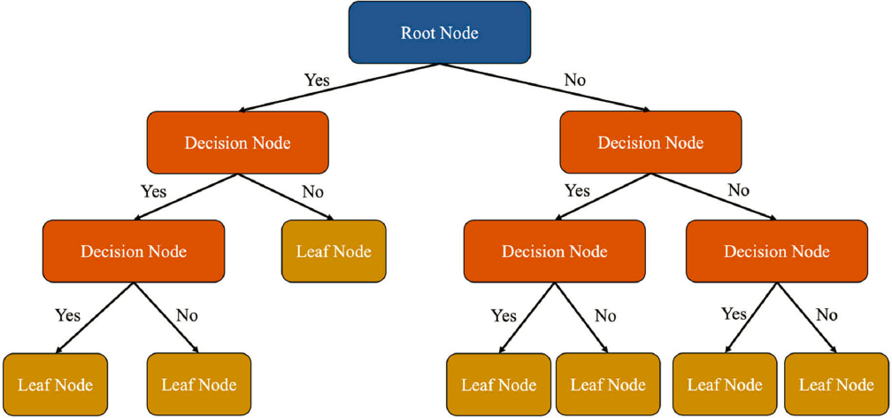
This method used a supervised ML classification technique, called decision trees, to assign sample counts, extracted from CCSs, to clusters based on one or more common attributes. DTs create a tree-like structure to make predictions for classification and regression tasks. Starting with a root node, the algorithm selects features and determines split points to create internal decision nodes. This splitting process continues until a stopping criterion is met, resulting in leaf or terminal nodes representing final predictions. The advantages of a DT model are that it can accommodate both categorical and numerical data and the decision process can be interpreted visually. Figure 19 illustrates the main components of a DT.
The dataset used to develop and validate DTs was divided into a training set and a testing set. The training set included a target variable and independent variables. The target variable was the cluster membership of each sample count extracted from CCSs. In M14, six DTs were developed for each state and year using the following six independent variables, respectively:
- 8,760 HFs by day of year (= 24 hours × 365 days).
- 2,016 HFs by month and DOW (= 24 hours × 12 months × 7 DOWs).
- 1,008 two-hour factors by month and DOW (= twelve 2-hour intervals × 12 months × 7 DOWs).
- 672 three-hour factors by month and DOW (= eight 3-hour intervals × 12 months × 7 DOWs).
- 336 six-hour factors by month and DOW (= four 6-hour intervals × 12 months × 7 DOWs).
- Time-block (AM peak, noon off-peak, PM peak, night) factors by month and DOW (TBMDWFs) (= 4 time-blocks × 12 months × 7 DOWs).
Each DT was trained to assign counts to the k clusters (k∈[2, n/5]) developed in:
- M10 using 84 MDWFs.
- M13 using the 12 MFs.
- M13 using the 2,016 HFs by month and day of week.
For example, in 2019, 155 CCSs from Florida were used to run clustering (M10) 31 (max k = n/5 = 155/5) times; each time, a different number of k clusters was developed. Each of the six DTs listed above was applied to each set of k clusters generated in M10. Furthermore, the same six DTs were also applied to the 31 sets of clusters developed in M13 using the 12 MFs and separately to the 31 sets of clusters created in M13 using the 2,016 HFs. This resulted in a total of 558 DTs (= 6 DTs × 31 sets of k clusters × 3 clustering methods) for Florida in 2019. All accuracy metrics and success rates were separately calculated for each DT.
The testing set contained the sample counts of a single CCS, which had been removed from the training set. After a DT model was trained using the remaining CCSs within a state and year, the model was applied on the testing set to assign the sample counts of the single CCS that had not been used in the training set. This process was repeated for every CCS from which sample counts were extracted and validated.
Each DT compared the factors of each count against the corresponding factors of each cluster. In the case of sample counts, these factors were calculated only for the specific day from which each count was extracted, whereas in the case of clusters, the factors were calculated for all days within a year. After the factors of a count were compared against the corresponding factors of every cluster, the count was assigned to the cluster exhibiting the most similar factors. To estimate the AADT of each sample count, its daily volume was multiplied with the corresponding group adjustment factor of the cluster to which the count was assigned by the DT.
The validation of the DTs involved determining not just the accuracy of the AADT estimates derived from the factored counts but also the success rate (percent) of each DT. The success rate was determined as the ratio of the number of counts that were correctly assigned to the cluster containing the parent CCS of each sample count to the total number of sample counts assigned to clusters.
M15—Assignment of SDCs to Clusters Using SVMs
Support vector machines are a supervised machine learning method suitable for classification and prediction tasks. It uses a kernel function to transform non-linearly separated data from an input space to a feature space, where the data are separated linearly. Then, they are transformed back to the input space, where they become again nonlinear.
In M15, SVMs were used to assign a count to a cluster. All the steps of the model development and validation process were identical to those followed in M14. This includes using the same six assignment attributes to develop six SVMs per state and year and assigning counts to the same clusters that were developed in M10 and M13 using 84 MDWFs (M10), 12 MFs (M13), and 2,016 HFs (M13). In other words, the only difference between M14 and M15 is that
the latter involved developing SVMs instead of DTs. Similar to M14, the validation of the SVMs included determining the accuracy of the AADT estimates derived from factored counts and the success rate (percent) of the assignments performed by the SVMs.
NEW METHODS
Table 19 presents four new methods that were examined in this project. These methods are applicable to all roadway functional classes.
Table 19. New Methods.
| No. | Method | Description and Rationale for Selecting Each Method | |
|---|---|---|---|
| M16 | Apply alternative methods to assign SDCs to individual CCSs within the same functional class | DTs | DTs and SVMs were used to assign counts to individual CCSs within a functional class. The aforementioned assignment methods have been used in previous works, produced promising results, and are also available in statistical programs and languages. |
| M17 | SVMs | ||
| M18 | Annualize SDCs using probe-based adjustment factors | All vehicle classes together | Annualized counts by applying segment-specific adjustment factors developed from raw uncalibrated probe data. Method 18 involved developing probe-based adjustment factors for all vehicle classes as one group, whereas in Method 19 probe-based adjustment factors were separately developed for groups of vehicle classes. M18 and M19 eliminate the need to create factor groups and assign counts to these groups. |
| M19 | Different vehicle classes | ||
M16 (DTs) and M17 (SVMs) involved assigning a sample count extracted from a CCS to another CCS within the same FC based on some common temporal and spatial attributes such as those described previously. This was necessary to determine if these variables could be used to effectively identify an individual CCS that exhibits similar traffic patterns with those at the sample count location as opposed to using average group adjustment factors produced from many CCSs that may be highly heterogeneous.
Note that M16 and M17 are “base” versions of CCS-specific assignment approaches and come with some limitations. For example, one limitation is that if a CCS does not collect data for some period, the counts originally assigned to the CCS have to be assigned to a different CCS. Further, M16 and M17 permit the assignment of counts to any CCS within the same FC regardless of their distance. However, if a count is far away from the assigned CCS, and the traffic patterns at the CCS location are affected by unusual local events, the accuracy of the AADT estimate derived from the factored count be compromised. These issues may be alleviated by annually assigning counts to CCSs and/or incorporating geographical constraints into these methods.
The main advantages of probe-based factors (M18 and M19) over other grouping and assignment methods include a) the ability to develop one or more sets of probe-based factors separately for every roadway segment of the entire network; b) the elimination of the need to create seasonal adjustment factor groups; and c) the elimination of the need to assign counts to factor groups.
M16—Assignment of Counts to Individual CCSs Using DTs
In M16, DTs were employed to assign sample counts extracted from a single CCS to another CCS within the same FC. Similar to M14, six DTs were developed for each state and
year using the same six assignment attributes (i.e., temporal adjustment factors) that were described in M14. The DTs compared the adjustment factors calculated for each count against the corresponding factors calculated for each CCS that belonged to the same FC as the parent CCS of the count. After all comparisons were performed, each count was assigned to the CCS exhibiting the most similar factors.
M17—Assignment of Counts to Individual CCSs Using SVMs
The only difference between M16 and M17 was that in the latter, SVMs were used instead of DTs. The assignment attributes and the model validation process were identical.
M18—Annualization of SDCs Using Probe-Based Factors for Total Traffic
M18 and M19 included annualizing sample counts by applying segment-specific adjustment factors developed from raw unadjusted probe count data that were provided by three vendors. In M18, probe-based adjustment factors were developed for all 13 FHWA vehicle classes combined into a single group of vehicles. In other words, there was no differentiation between motorcycles, cars, buses, and trucks. For each CCS location examined in this study (see Study Data section), the raw probe trip counts were used to calculate, where applicable, the following average probe counts and adjustment factors:
- Average probe counts:
- 1 annual average daily probe count (AADPC).
- 7 annual average day-of-week probe counts (AADWPCs).
- 12 monthly average daily probe counts (MADPCs).
- 84 monthly average day-of-week probe counts (MADWPCs).
- 365 average daily probe counts (ADPCs).
- Probe-based adjustment factors:
- 7 annual day-of-week factors (=AADPC/AADWPC).
- 12 monthly factors (=AADPC/MADPC).
- 84 monthly day-of-week factors (=AADPC/MADWPC).
- 365 daily factors (=AADPC/ADPC).
In the case of one of the three vendors, the raw probe trip counts were obtained at a monthly aggregation, so only the 12 monthly adjustment factors could be calculated. For the other two vendors, all four sets of adjustment factors were calculated. Each set of probe-based adjustment factors was validated as follows. Sample counts were extracted from each CCS and were factored by multiplying the actual ADT of each count by the corresponding probe-based adjustment factor calculated for that CCS location. The probe-based AADT estimates were then compared against the actual AADT of each CCS. This comparison involved the calculation of the same performance metrics that were used to validate Methods 1–17. These metrics are presented in the Validation section.
In addition to the validation of the probe-based adjustment factors, M18 involved determining penetration rates of the probe data. First, the penetration rate of each vendor’s probe data was calculated for each CCS location as follows:
Where:
PRi = penetration rate of probe data at CCS i.
d = day of year (1, 2,…365 or 366 in leap years).
dmax = total number of days in a year (365 or 366 in leap years). dmax
ADTd,i = average daily traffic at CCS i on day-of-year d.
ADPCd,i = average daily probe count at the location of CCS i on day-of-year d.
After determining the penetration rate per CCS, average penetration rates were calculated by vendor, state, FC, RU, FC_RU, and volume group. Further, M18 involved determining the Pearson correlation coefficient between each set of probe-based adjustment factors and the corresponding actual adjustment factors calculated from CCS data.
M19—Annualization of SDCs Using Probe-Based Factors for Truck Traffic
In this method, probe-based adjustment factors were separately developed for two groups of vehicle classes that included medium-duty (vehicle classes 4–6) and heavy-duty vehicles (classes 7–13). Raw probe monthly trip counts for different vehicle classes were only available from one vendor for the state of Minnesota. These data were used to calculate 12 monthly adjustment factors at each classification site. The procedure for calculating AADT estimates and validating the probe-based factors was the same as that in M18. Penetration rates were determined as a ratio of the sum of the 12 MADPCs to the sum of the 365 ADT values. Further, correlations were determined between the 12 monthly probe-based adjustment factors and the corresponding MFs derived from CCS data.
More information about the probe data that were used in this project is provided in Chapter 5.
VALIDATION
The validation of the methods described in the previous section involved determining, where applicable, the following key performance elements associated with the factor groups created by each method during the ‘grouping’ step, and the AADT estimates produced by each method during the ‘assignment’ step:
Factor Groups:
- Within-group variability. It captures the internal homogeneity of the adjustment factor groups in terms of the monthly day-of-week patterns of the CCSs included in each group. The more similar the traffic patterns, the lower the variability. The coefficient of variation was used to capture the amount of variability of each group adjustment factor.
- Precision of group adjustment factors. It reflects the consistency of the CCSs’ individual adjustment factors that were used to calculate a group adjustment factor. The precision is described in the TMG. It accounts not only for the coefficient of variation of each group adjustment factor, but also for the sample size (i.e., number of CCSs) of a group.
AADT Estimates:
- AADT accuracy. It captures the closeness between the actual AADTs calculated using CCS data and the AADT estimates derived from annualized sample counts.
- AADT precision. It indicates how close the AADT estimation errors are. The closer the errors, the higher the precision, and vice versa.
The AADT accuracy and precision are more important than the within-group variability and the precision of group factors because ultimately, many applications (e.g., pavement design, environmental analysis, safety analysis, etc.) where AADT estimates are being used produce results that are as good as the accuracy of the inputs (i.e., AADT estimates); however, quantifying and considering all four elements associated with each method facilitates method comparisons, providing a more complete understanding of each method’s performance. The four key elements are described in the sections that follow.
Within-Group Variability
Some of the methods described in the previous section (M2–M13) involve developing groups of CCSs (i.e., adjustment factor groups) based on one or more common attributes. According to the literature, some methods such as cluster analysis produce more homogeneous groups of CCSs in terms of temporal travel patterns than others. The more similar the travel patterns of the CCSs within a group, the lower the within-group variability, indicating greater internal homogeneity within the group. To quantify the overall variability of all factor groups created by each method, a weighted average coefficient of variation (WACV) was computed following three steps. The first step was to calculate the coefficient of variation (CV) of each group monthly day-of-week adjustment factor from the corresponding individual (monthly day-of-week) adjustment factors of the CCSs within the group. The coefficient of variation of each group factor was calculated as follows:
Where:
CVm,j,k = coefficient of variation of group adjustment factor for month m and day-of-week j in group k.
Sm,j = sample standard deviation of the CCSs’ individual adjustment factors for month m sm,j and day-of-week j in group (or cluster in the case of cluster analysis) k.
= average monthly day-of-week adjustment factor of group k for month m and day-of-week j.
The first step yielded 84 monthly day-of-week CVs for each group k created using a specific grouping method. In the second step, the average coefficient of variation (ACV) was calculated for each group as a simple average of the 84 CVs calculated in the first step:
In the third step, a WACV was calculated for all groups created by each method by accounting for the number of CCSs within each group.
Where:
WACV = weighted average coefficient of variation of all groups developed using a specific grouping method. The lower the WACV, the more homogeneous the groups of a method.
nk = total number of CCSs within group k.
ng = total number of groups or clusters developed using a specific method.
Group Adjustment Factor Precision
The precision of a specific group adjustment factor reflects the consistency of the CCS’s individual adjustment factors that were used to calculate the group factor. The precision of each group monthly day-of-week adjustment factor was calculated based on the assumption stated in the TMG that the existing CCSs “are equivalent to a simple random sample selection” (FHWA 2022):
Where:
Pm,j,k = precision interval as a percentage of the group factor for month m and day-of-week j in group k.
t = value of Student’s T-distribution with 1−α/2 level of confidence and n−1 degrees of freedom.
α = significance level (0.05) for 95 percent confidence (α = 1–0.95).
For more information on the precision of group adjustment factors, see the TMG (FHWA 2022). The formula above can be used to estimate the sample size needed to achieve any desired precision level. Tight precision levels (i.e., low precision values) require large sample sizes, leading to expensive programs. On the other hand, loose precision levels (i.e., higher precision values) require fewer CCSs but result in less-precise factors. According to the TMG, the recommended precision level for a group monthly adjustment factor is ±10 percent with 95 percent confidence, with the exception of recreational groups, for which no target precision is specified (under ±25 percent is desired).
After estimating the precision of each group factor, the average precision (AP) of each group was calculated as follows.
In the last step, a weighted average precision (WAP) was calculated for all groups created by each method by accounting for the number of CCSs within each group.
AADT Accuracy
The AADT accuracy pertains to how close an AADT estimate is to the actual AADT. The closer the two AADT values are, the higher the AADT accuracy, or the lower the AADT estimation error. In this project, the actual AADTs are calculated from CCS data, whereas the estimated AADTs are derived from 24-hour sample counts extracted from CCSs and annualized using the adjustment factors developed by a grouping/assignment method.
The LOO approach was used to validate all existing, improved, and new assignment methods except for M18 and M19, which were validated using a slightly different approach, as described in the previous section. The LOO approach was used in the majority of the studies presented in Chapter 2. In this project, it was applied separately for each state and year following the steps described below:
- Step 1: Extracted all available sample 24-hour counts from each CCS. Days within holiday periods were excluded from the validation because they often exhibit atypical traffic volumes and patterns. Appendix C includes a table that lists all federal holiday periods that were excluded from the validation. Each sample count included in the validation dataset was treated as a test count. The parent CCS from which sample counts were extracted was excluded from the analysis to avoid potential bias caused by correlations between estimated and actual AADTs. All CCSs from 45 states (see Chapter 5) were used to simulate and validate sample counts.
- Step 2: Annualized each sample count using one assignment method at a time. An AADT was estimated from each factored count after multiplying the ADT of the count by an appropriate adjustment factor. As previously mentioned, this step was not performed in the case of the no-factoring method (M1).
-
Step 3: Calculated the following performance metrics (i.e., errors) for every pair of estimated AADT (AADTEst) and actual AADT (AADTAct) of each CCS:
- Algebraic (Signed) Difference: AD = AADTEst − AADTAct
- Percent Error: PE = 100 × (AADTEst − AADTAct)/AADTAct
- Absolute Percent Error: APE = 100 × |(AADTEst − AADTAct)|/AADTAct
- Coefficient of Variation: CV = 100 × (2 × |AADTEst − AADTAct|)/(AADTEst + AADTAct)
-
Step 4: Determined the following descriptive statistics for each metric calculated in Step 3:
- Total number of sample counts.
- Total number of CCSs.
- Mean.
- Median.
- Standard deviation.
- 2.5th and 97.5th percentiles.
Initially, the descriptive statistics were separately calculated for each state and year using sample counts from all five weekdays, Monday through Friday, because 80 percent of the states that responded to the survey indicated that they conduct counts only on weekdays.
-
Step 5: Repeated Step 4 by calculating the descriptive statistics listed above at different levels of aggregation, if applicable:
- By state (all three years from each state were combined).
- FC.
- FC_RU.
- Five volume groups.
- Ten volume groups.
- Nationwide, across all 135 state-year combinations (= 45 states × 3 years).
-
Step 6: Repeated Steps 4 and 5 by calculating the descriptive statistics using sample counts from four additional day-of-week groups:
- Tuesday through Thursday.
- Saturday and Sunday.
- Friday, Saturday, and Sunday.
- Monday through Sunday.
In addition, statistical t-tests, assuming unequal variances, were conducted to test whether the mean errors of any pair of methods examined in this study were statistically different at the 95 percent confidence level.
AADT Precision
The AADT precision reflects the closeness among AADT estimation errors. The closer the errors, the tighter the precision (i.e., low precision values), and vice versa. The AADT precision can be captured using several of the metrics and descriptive statistics listed above such as the standard deviation of the PEs. Another precision metric is the difference between the 97.5th and the 2.5th percentiles of the PEs. This difference captures the range or interval within which 95% of the entire population of AADT errors is expected to fall. The narrower the interval, the more precise the AADT estimates.


