Methods for Assigning Short-Duration Traffic Volume Counts to Adjustment Factor Groups to Estimate AADT (2024)
Chapter: 6 Results
CHAPTER 6. RESULTS
This chapter presents the results from the validation of the existing, improved, and new assignment methods described in Chapter 4.
EXISTING METHODS (M1–M9)
As explained in Chapter 4, various performance metrics were aggregated at different levels using sample counts extracted from different days of the week. Figure 20 shows the overall AADT accuracy at the national level of five existing methods applied to all FCs. In particular, Figure 20a and Figure 20b show the median PE and the MAPE, respectively, of methods M1–M5 that were applied and validated using data from over 9,700 CCSs located on all FCs across all 135 state-year combinations (= 45 states × 3 years) examined in this study. The five colored bars plotted for each method show the errors obtained for the five day-of-week groups from which sample counts were extracted. In both figures, the standard deviation of each aggregate error is depicted on every bar as a black vertical line.
In Figure 20a, the median PE captures the AADT bias—positive values suggest that the AADT estimates are overestimated, negative values indicate underestimation of AADT, and values close to zero suggest low bias. Though the median PE can help to understand whether a method consistently underestimates or overestimates AADT, it does not capture the magnitude of the errors associated with each method. For this reason, the MAPE is plotted in Figure 20b.
The main observations from Figure 20a are:
- Not factoring counts (M1) results in a significant overestimation (positive errors) of AADT if counts are taken on weekdays and underestimation (negative errors) of AADT when counts are conducted on Saturday or Sunday. This can be attributed to the fact that the average weekend traffic on nonrecreational roads tends to be lower than the AADT.
- The remaining four methods (M2, M3, M4, M5) slightly overestimate AADT regardless of the days of the week on which the counts are taken.
- Not surprisingly, in all cases, the standard deviations are high due to the aggregation of the results at the national level. Appendix E shows the main results disaggregated by state.

The main findings from Figure 20b are:
- Among the five methods, not factoring counts (M1) yields the least accurate AADT estimates in all five day-of-week groups. The MAPE of M1 ranges from 11.5 percent (for counts taken on Tuesday–Thursday) to 19.1 percent (for counts conducted on Saturdays and Sundays).
- Unfactored counts taken between Tuesday and Thursday result in significantly lower errors than unfactored counts taken over the weekend. As noted previously, this can be explained by the fact that midweek traffic volumes—as opposed to weekend volumes—on nonrecreational roads tend to be more representative of AADT.
- One difference between M1 and the other methods is that unfactored counts (M1) taken between Tuesday and Thursday (orange bar) produce slightly lower errors than unfactored counts conducted between Monday and Friday (blue bar); however, the opposite trend is consistently observed in the case of M2 through M5.
- Among all methods, M3 (FC_RU) produced the most accurate AADTs in all five day-of-week groups across all 45 states. The t-tests showed that the MAPEs of M3 are statistically different than the errors of the other methods at the 95 percent confidence level; however, the average difference in MAPEs between M3 and each of the other methods is only 0.5 percent. It is worth noting, nonetheless, that there is a high variability in these results at the state level. For example, in many states, FC_RU tends to be a more accurate grouping approach than using only FC. However, in some states, both variables result in similar levels of AADT accuracy.
- Splitting five volume groups (M4) into 10 volume groups (M5) did not improve AADT accuracy. This suggests that seasonal traffic patterns do not significantly change among the smaller volume groups of M5. However, as previously mentioned, these results exhibit high variability. Appendix E provides results aggregated by state.
Figure 21a and Figure 21b show the median PE and the MAPE, respectively, of seven existing methods that were validated using CCSs located on FC6 and FC7 in (up to) 58 state and year combinations. The main findings from Figure 21a are:
- Counts taken on weekdays (Monday–Friday) overestimate AADT, particularly those that have not been factored (median APE = 7.9 percent).
- With the exception of M2 and M3, the remaining methods underestimate AADT when counts are conducted over the weekend.
- For counts taken on all seven days of the week, Monday through Sunday, the smallest biases are produced by M3 (median PE = 1.0 percent) and M2 (median PE = 1.2 percent), and the highest errors are associated with M1 (median PE = 3.3 percent).
- Not surprisingly, there is a high variability in all errors, indicating that the results may vary or significantly vary from one state to another.
The following observations can be made from Figure 21b:
- Unfactored counts (M1) taken on Saturday or Sunday (gray bars) produce the least accurate AADT estimates (MAPE = 21.4 percent).
- In the case of midweek counts taken between Tuesday and Thursday (orange bars), the worst performing method is M7 (MAPE = 14.0 percent), followed by M6 (MAPE = 13.4 percent) and M1 (MAPE = 13.2 percent). In other words, applying factors from FC5 to (midweek) counts on FC6 and FC7 results in less accurate AADTs than not factoring the counts at all.
- M6 yields slightly more accurate AADTs than M1 when counts are taken between Monday and Friday (blue bars).
- In the case of weekday counts (Monday–Friday), the best performing methods are M3 (MAPE = 11.8 percent) and M2 (MAPE = 11.9 percent). The t-tests showed that the MAPEs of M3 (FC_RU) are statistically different than the errors of M2 (FC) at the 95 percent confidence level; however, the average difference in their MAPEs is negligible (0.1 percent).
- M4 (5_VG) and M5 (10_VG) yielded slightly higher errors than M2 (FC) and M3 (FC_RU).
- Splitting five volume groups (M4) into 10 volume groups (M5) did not provide any significant improvement in AADT accuracy.
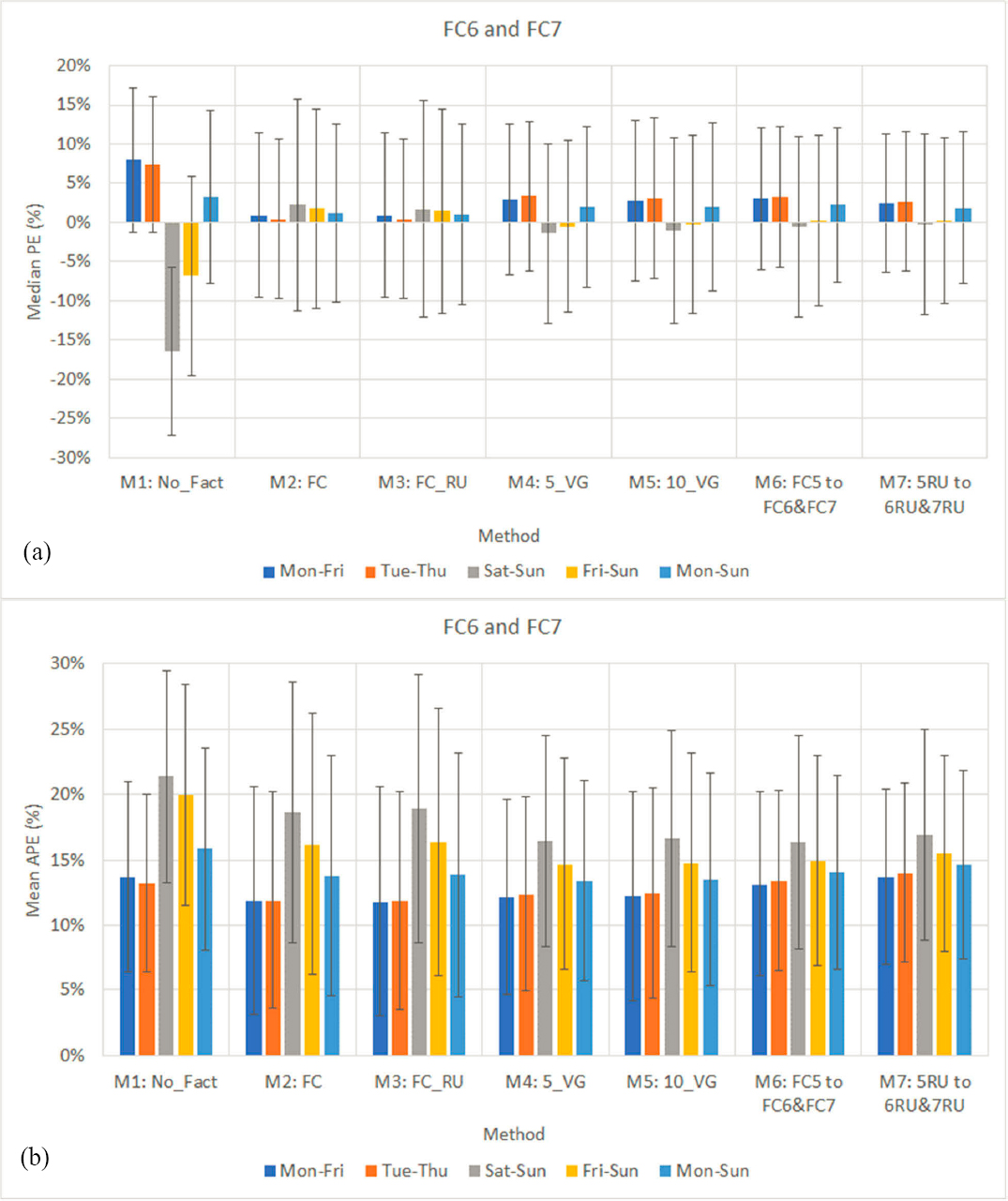
Figure 22a and Figure 22b show the median PE and the MAPE, respectively, of seven existing methods validated using sample counts extracted from FC6 in (up to) 42 state-years. The main findings from Figure 22a are provided below:
- Counts taken on weekdays (Monday–Friday) tend to overestimate AADT, particularly those that have not been factored (median APE=6.7 percent). The smallest biases are produced by M2 (1.2 percent) and M3 (1.2 percent).
- For counts taken on all seven days of the week, Monday through Sunday, the smallest biases are produced by M2 (1.0 percent) and M3 (1.0 percent). M1 yields the highest errors (2.4 percent).
- When counts are conducted over the weekend, M1 (No_Fact) significantly underestimates AADT (-14.0 percent). Most of the remaining methods slightly overestimate AADT.
The following observations can be made from Figure 23b:
- Since no stations belong to 6U, the results generated by M2 (FC) and M3 (FC_RU) are identical.
- In the case of weekday counts (Monday–Friday), the best performing methods are M4 (12.0 percent) and M5 (12.0 percent) followed closely by M2 and M3 (12.6 percent), and then by M6 (13.1 percent). M1 produces the least accurate AADT estimates (14.2 percent).
- In the case of weekend counts (Saturday–Sunday), the most accurate AADTs (15.1 percent) are obtained from M4 and the least accurate are produced by M1 (19.7 percent). M4 (15.1 percent) and M5 (15.4 percent) yielded slightly lower errors than M2 and M3 (16.6 percent). Moreover, splitting five volume groups (M4) into ten volume groups (M5) slightly decreased AADT estimation accuracy (15.4 percent).
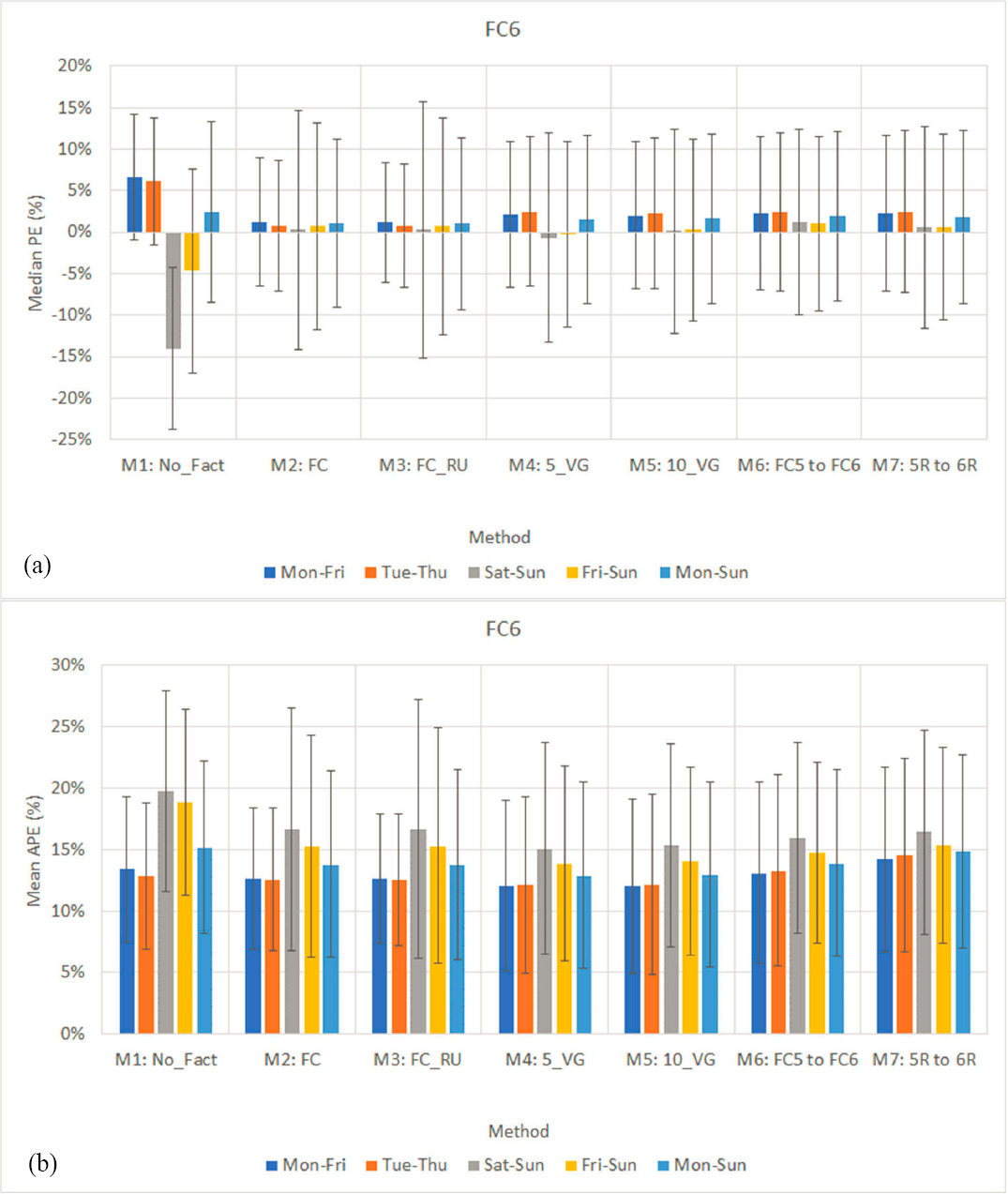
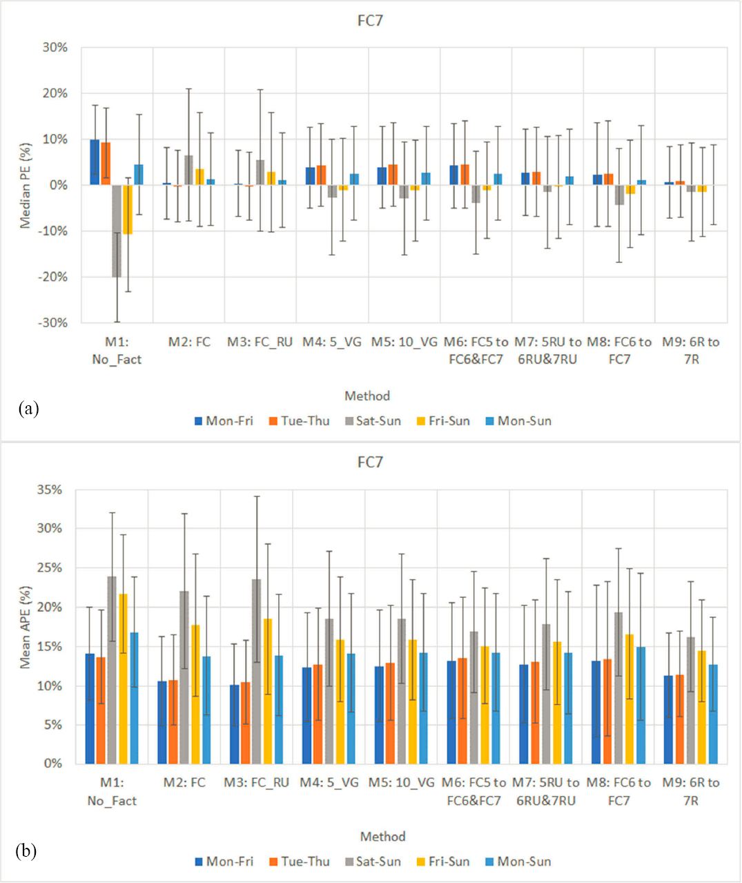
Figure 23a and Figure 23b show the median PE and the MAPE, respectively, of all nine existing methods validated using sample counts extracted from FC7 in 28 state-years. The main findings from Figure 23a are:
- Counts taken on weekdays (Monday–Friday) tend to overestimate AADT, particularly those that have not been factored (median APE = 10.0 percent). The smallest biases are produced by M3 (0.4 percent), M2 (0.5 percent), and M9 (0.7 percent).
- For counts taken on all seven days of the week, Monday through Sunday, the smallest biases are produced by M9 (0.2 percent), M3 (1.1 percent), and M8 (1.2 percent). M1 yields the highest errors (4.6 percent).
- With the exception of M2 (FC) and M3 (FC_RU), the remaining methods underestimate AADT when counts are conducted over the weekend.
- Not surprisingly, there is a high variability in all errors.
The following observations can be made from Figure 23b:
- In the case of weekday counts (Monday–Friday), the best performing methods are M3 (10.1 percent), M2 (10.6 percent), and M9 (11.3 percent). The t-tests showed that the MAPEs of M3 (FC_RU) are statistically different than the errors of M2 and M9 at the 95 percent confidence level; however, the differences in their MAPEs are small. In other words, if permanent sites do not exist on FC7, applying factors from 6R and 6U to counts on 7R and 7U, respectively, produces AADT estimates that are almost as accurate as when factors are applied from the same FC (M2) or FC_RU (M3). In addition, M9 produces significantly more accurate AADT estimates than M6–M8, which means that annualizing counts on local roads using factors from 6R and 6U is a more effective approach than using factors developed for FC5, 5R, 5U, or FC6. Further, M1 produces the least accurate AADTs (14.1 percent).
- The results from the validation of midweek counts (Tuesday and Thursday) are similar to those described above for weekday counts (Monday–Friday).
- In the case of weekend counts, the most accurate AADTs (16.3 percent) are obtained from M9 and the least accurate are produced by M1 (23.9 percent).
- M4 (5_VG) and M5 (10_VG) yielded slightly higher errors than M2 (FC) and M3 (FC_RU).
- Splitting five volume groups (M4) into 10 volume groups (M5) did not provide any significant improvement in AADT accuracy.
For completeness, the AADT accuracy of each method needed to be examined in combination with the other performance metrics presented in Chapter 4, such as the WACV and the precision of the group factors. Table 24 shows the most important aggregate performance metrics of the existing methods at the national level. The validation results are separately
provided for the analyses conducted using weekday sample counts (Monday–Friday) extracted from CCSs located on (a) all FCs, (b) FC6, and (c) FC7. The fifth column shows the average number of CCSs per group, and the last three columns show the total number of state-years, the total number of CCSs, and the total number of sample counts used in this validation. The validation results from weekday counts (Mon–Fri) are presented here; however, Appendix D shows the results stemming from the validation of counts extracted from the other four day-of-week groups (Tue–Thu, Sat–Sun, Fri–Sun, and Mon–Sun) examined in this study.
Table 24. Performance Metrics of Existing Methods across All States and Years for Different FC Groups (Mon–Fri).
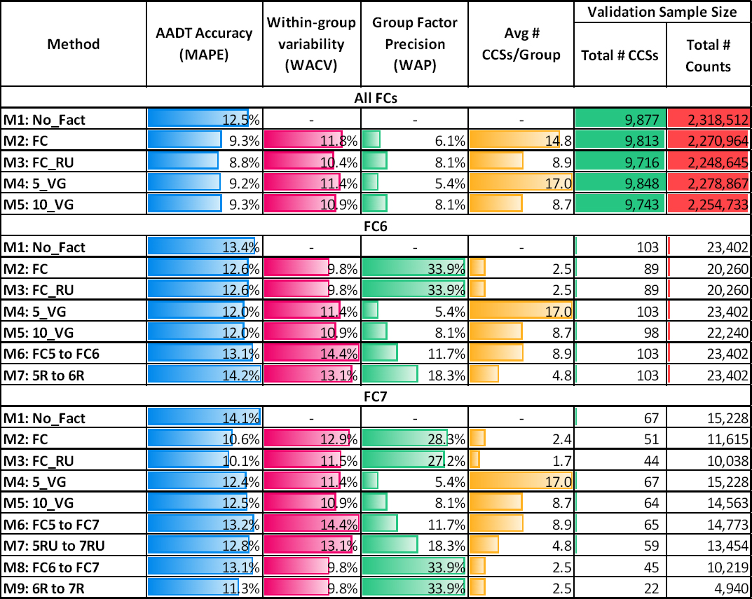
The main findings from Table 24 are as follows:
- All FCSs:
- The WACV tends to decrease as the number of CCSs within a group decreases, and vice versa. For example, M2 (FC) produces up to seven factor groups per state and year, with each group containing on average 14.8 CCSs. M3 (FC_RU), on the other hand, results in up to 14 smaller groups per state and year, with each group containing on average 8.9 CCSs. The smaller groups of M3 are on average more homogeneous (WACV = 10.4
- percent) than the bigger groups of M2 (WACV = 11.8 percent). In this example, M3 also produces more accurate AADTs (MAPE = 8.8 percent) than M2 (MAPE = 9.3 percent); however, splitting a group into subgroups based on the same variable does not necessarily improve the AADT accuracy, as explained below.
- The five volume groups of M4 are bigger in size and less homogeneous (WACV = 11.4 percent) than the 10 smaller volume groups produced by M5 (WACV = 10.9 percent); however, M4 results in slightly lower MAPEs than M5. This suggests that beyond a certain critical point, creating more volume groups does not significantly improve the AADT accuracy even though the within-group variability continues to decrease. This happens because each volume group can contain highly variable monthly day-of-week patterns/factors, which depend on various spatiotemporal characteristics, not just the volume of each CCS. In general, a grouping variable (e.g., FC in M2 or volume in M4 and M5) can only capture some of the variability in the CCSs’ monthly day-of-week patterns. This finding is further discussed and illustrated in the next section, which presents the results from cluster analysis.
- With a few exceptions, the MAPE generally exhibits similar trends to the WACV, but opposite trends compared to the WAP. In other words, as MAPE decreases, the WACV tends to decrease, while WAP tends to increase. This makes the interpretation of the WACV results more intuitive than those of the precision. For example, M3 is more accurate and produces more homogeneous groups than M2, yet M2 yields more precise factors (6.1 percent) than M3 (8.1 percent) because it contains more CCSs per group.
- FC6:
- Since no CCSs were available on 6U, the results generated by M2 (FC) and M3 (FC_RU) are identical and are based only on validated sample counts on 6R.
- The most accurate methods are volume groups, M4 and M5 (MAPE = 12.0 percent), followed by M2 and M3 (MAPE = 12.6 percent).
- Splitting 5 volume groups into 10 volume groups does not improve AADT accuracy. Note that the volume groups in M4 and M5 include CCSs from all FCs, not just from FC6, which is why the average number of CCSs/group is relatively high and the WAP is low compared to those of M2 and M3, which include CCSs only from FC6.
- M7 yields the least accurate AADT estimates (MAPE = 14.2 percent). M6 (MAPE = 13.1 percent) does not produce better results than M2-M5 either. This suggests that annualizing counts conducted on FC6 using factors from FC5 does not improve AADT accuracy.
- FC7:
- The most accurate methods are FC_RU (10.1 percent) and FC (10.6 percent), followed by M9 (11.3 percent), which involved annualizing counts conducted on 7R using factors from 6R (no CCSs were available on 6U).
- Not factoring weekday counts (M1) results in the least accurate AADTs (14.1 percent).
- M9 tends to be more accurate than M8 because in the latter, factors from 6R are applied to counts taken on both 7R and 7U, whereas in M9, factors from 6R are applied to counts only on 7R. This confirms that accounting for the area type (i.e., rural vs. urban) in the factor grouping process tends to improve AADT accuracy. M8 and M9 have the same WACV, WAP, and average number of CCSs/group because the factor groups in both methods contain the same CCSs within 6R.
For completeness, Table 25 and Table 26 show various statistics aggregated across all 135 state-years for methods M1 through M5 that were applied to all functional classes. For each method, the statistics are separately provided for the five day-of-week groups (Monday–Friday, Tuesday–Thursday, Saturday–Sunday, Friday–Sunday, Monday–Sunday) from which sample counts were extracted and validated. Similar results were obtained for all methods examined this project.
Table 25. Aggregated Results across All 135 State-Years for M1 M2 and M3
| Metric | M1: No Factoring | M2: FC | M3: FCRU | |||||||||||||
|---|---|---|---|---|---|---|---|---|---|---|---|---|---|---|---|---|
| Mon–Fri | Tue–Thu | Sat–Sun | Fri–Sun | Mon–Sun | Mon–Fri | Tue–Thu | Sat–Sun | Fri–Sun | Mon–Sun | Mon–Fri | Tue–Thu | Sat–Sun | Fri–Sun | Mon–Sun | ||
| AD | Mean | 1386.4 | 1012.0 | -3246.9 | -951.5 | 74.2 | 538.3 | 607.9 | 265.8 | 238.9 | 461.1 | 314.2 | 305.6 | 572.1 | 447.4 | 387.2 |
| Med. | 449.1 | 334.7 | -1029.0 | -155.3 | 125.4 | 67.0 | 66.9 | 37.8 | 40.1 | 60.7 | 55.7 | 51.4 | 37.2 | 39.8 | 51.8 | |
| StD. | 5174.4 | 4868.2 | 7960.7 | 8069.7 | 6441.8 | 5160.0 | 5186.5 | 8296.0 | 7364.0 | 6212.3 | 5299.0 | 5234.9 | 9272.9 | 8190.5 | 6670.3 | |
| 2.5th | -5660.4 | -6077.9 | -24783.4 | -20402.9 | -13183.8 | -5400.4 | -5367.6 | -11485.6 | -9896.8 | -7242.0 | -5420.2 | -5527.6 | -9284.3 | -8157.9 | -6558.8 | |
| 97.5th | 13501.9 | 11952.2 | 6365.2 | 13699.4 | 12186.5 | 9485.2 | 10146.6 | 12314.5 | 10711.7 | 10374.1 | 7556.3 | 7729.9 | 12860.8 | 10968.5 | 9206.7 | |
| PE | Mean | 4.9% | 3.1% | -11.3% | -2.6% | 0.3% | 1.6% | 1.5% | 3.0% | 2.5% | 2.0% | 1.4% | 1.4% | 2.6% | 2.2% | 1.8% |
| Med. | 6.0% | 4.9% | -12.9% | -3.5% | 2.4% | 1.2% | 1.2% | 0.7% | 0.7% | 1.1% | 0.9% | 0.9% | 0.7% | 0.7% | 0.9% | |
| StD. | 16.5% | 15.6% | 22.5% | 24.1% | 19.8% | 14.5% | 14.7% | 23.0% | 20.5% | 17.3% | 14.6% | 14.8% | 22.6% | 20.2% | 17.3% | |
| 2.5th | -31.0% | -32.2% | -47.9% | -44.7% | -40.7% | -25.2% | -25.9% | -32.1% | -29.9% | -27.9% | -24.1% | -24.7% | -31.5% | -29.4% | -27.1% | |
| 97.5th | 34.3% | 28.5% | 39.7% | 43.4% | 35.4% | 29.5% | 29.8% | 50.8% | 44.9% | 36.7% | 28.1% | 28.4% | 46.7% | 41.6% | 34.4% | |
| APE | Mean | 12.5% | 11.5% | 19.5% | 19.1% | 14.5% | 9.3% | 9.4% | 14.7% | 12.6% | 10.8% | 8.8% | 8.9% | 13.9% | 12.1% | 10.3% |
| Med. | 9.8% | 9.0% | 16.6% | 16.5% | 11.2% | 6.2% | 6.4% | 10.2% | 8.3% | 7.1% | 5.8% | 5.8% | 9.7% | 8.0% | 6.6% | |
| StD. | 11.9% | 11.1% | 15.9% | 15.0% | 13.5% | 11.3% | 11.3% | 18.0% | 16.3% | 13.7% | 11.8% | 11.9% | 18.0% | 16.3% | 14.0% | |
| 2.5th | 0.5% | 0.5% | 0.8% | 0.9% | 0.5% | 0.3% | 0.3% | 0.5% | 0.4% | 0.3% | 0.3% | 0.3% | 0.4% | 0.3% | 0.3% | |
| 97.5th | 42.4% | 39.7% | 55.0% | 53.4% | 47.6% | 36.8% | 37.4% | 54.6% | 49.6% | 43.2% | 35.8% | 36.4% | 51.2% | 46.8% | 41.4% | |
| CV | Mean | 8.7% | 8.1% | 15.3% | 14.1% | 10.6% | 6.5% | 6.6% | 9.9% | 8.6% | 7.5% | 6.2% | 6.3% | 9.5% | 8.2% | 7.1% |
| Med. | 6.8% | 6.2% | 12.4% | 11.5% | 7.8% | 4.4% | 4.5% | 7.2% | 5.9% | 5.0% | 4.1% | 4.1% | 6.8% | 5.6% | 4.7% | |
| StD. | 8.7% | 8.6% | 12.8% | 11.5% | 10.5% | 7.8% | 7.9% | 10.0% | 9.4% | 8.6% | 7.6% | 7.8% | 9.7% | 9.1% | 8.4% | |
| 2.5th | 0.3% | 0.3% | 0.6% | 0.6% | 0.4% | 0.2% | 0.2% | 0.3% | 0.3% | 0.2% | 0.2% | 0.2% | 0.3% | 0.2% | 0.2% | |
| 97.5th | 30.2% | 29.9% | 46.0% | 42.7% | 38.0% | 25.7% | 26.2% | 35.6% | 32.9% | 29.6% | 25.1% | 25.6% | 34.3% | 31.7% | 28.7% | |
| # Sample Counts | 2,285,524 | 1,409,292 | 903,045 | 1,355,078 | 3,188,569 | 2,270,964 | 1,400,326 | 897,272 | 1,346,404 | 3,168,236 | 2,248,645 | 1,386,561 | 888,486 | 1,333,172 | 3,137,131 | |
| # CCSs | 9,877 | 9,877 | 9,877 | 9,877 | 9,877 | 9,813 | 9,813 | 9,813 | 9,813 | 9,813 | 9,716 | 9,716 | 9,716 | 9,716 | 9,716 | |
| Avg # of CCSs/Group | - | - | - | - | - | 14.8 | 14.8 | 14.8 | 14.8 | 14.8 | 8.9 | 8.9 | 8.9 | 8.9 | 8.9 | |
Table 26. Aggregated Results across All 135 State-Years for M4 and M5.
| Metric | M4: 5_VG | M5: 10_VG | |||||||||
|---|---|---|---|---|---|---|---|---|---|---|---|
| Mon–Fri | Tue–Thu | Sat–Sun | Fri–Sun | Mon–Sun | Mon–Fri | Tue–Thu | Sat–Sun | Fri–Sun | Mon–Sun | ||
| AD | Mean | 292.9 | 269.3 | 534.5 | 438.7 | 361.3 | 251.0 | 217.3 | 511.9 | 420.6 | 324.9 |
| Med. | 69.9 | 68.1 | 37.5 | 42.4 | 62.7 | 63.5 | 60.9 | 34.4 | 39.1 | 57.2 | |
| StD. | 4823.1 | 4826.3 | 8099.8 | 7161.2 | 5938.6 | 4596.6 | 4599.2 | 7623.2 | 6746.6 | 5622.9 | |
| 2.5th | -5819.2 | -6181.2 | -9682.9 | -8398.3 | -7087.1 | -5868.3 | -6268.4 | -9675.9 | -8345.9 | -7094.3 | |
| 97.5th | 7350.7 | 7457.4 | 13524.8 | 11473.4 | 9268.8 | 7204.6 | 7286.0 | 13512.5 | 11470.2 | 9155.6 | |
| PE | Mean | 1.6% | 1.5% | 3.1% | 2.5% | 2.0% | 1.5% | 1.5% | 3.1% | 2.5% | 2.0% |
| Med. | 1.2% | 1.2% | 0.7% | 0.8% | 1.1% | 1.1% | 1.0% | 0.7% | 0.7% | 1.0% | |
| StD. | 14.2% | 14.4% | 23.1% | 20.4% | 17.2% | 14.9% | 15.1% | 23.9% | 21.2% | 17.9% | |
| 2.5th | -24.8% | -25.5% | -32.3% | -29.9% | -27.6% | -24.9% | -25.6% | -33.1% | -30.6% | -28.0% | |
| 97.5th | 29.1% | 29.7% | 51.5% | 45.5% | 36.9% | 29.5% | 30.1% | 52.0% | 46.1% | 37.5% | |
| APE | Mean | 9.2% | 9.4% | 14.7% | 12.6% | 10.7% | 9.3% | 9.5% | 15.0% | 12.8% | 10.9% |
| Med. | 6.2% | 6.4% | 10.2% | 8.3% | 7.1% | 6.2% | 6.4% | 10.4% | 8.4% | 7.1% | |
| StD. | 11.0% | 11.0% | 18.0% | 16.3% | 13.6% | 11.7% | 11.8% | 18.9% | 17.1% | 14.3% | |
| 2.5th | 0.3% | 0.3% | 0.5% | 0.3% | 0.3% | 0.3% | 0.3% | 0.5% | 0.4% | 0.3% | |
| 97.5th | 36.1% | 36.8% | 54.9% | 49.7% | 43.1% | 36.6% | 37.4% | 55.4% | 50.3% | 43.8% | |
| CV | Mean | 6.4% | 6.6% | 10.0% | 8.6% | 7.4% | 6.5% | 6.7% | 10.1% | 8.7% | 7.5% |
| Med. | 4.4% | 4.5% | 7.2% | 5.9% | 5.0% | 4.4% | 4.5% | 7.3% | 5.9% | 5.0% | |
| StD. | 7.6% | 7.7% | 10.0% | 9.3% | 8.5% | 7.7% | 7.8% | 10.2% | 9.5% | 8.6% | |
| 2.5th | 0.2% | 0.2% | 0.3% | 0.2% | 0.2% | 0.2% | 0.2% | 0.3% | 0.2% | 0.2% | |
| 97.5th | 25.1% | 25.6% | 35.5% | 32.9% | 29.3% | 25.5% | 26.0% | 36.1% | 33.4% | 29.9% | |
| # Sample Counts | 2,278,867 | 1,405,195 | 900,436 | 1,351,139 | 3,179,303 | 2,254,733 | 1,390,302 | 890,910 | 1,336,838 | 3,145,643 | |
| # CCSs | 9,848 | 9,848 | 9,848 | 9,848 | 9,848 | 9,743 | 9,743 | 9,743 | 9,743 | 9,743 | |
| Avg # of CCSs/Group | 17.0 | 17.0 | 17.0 | 17.0 | 17.0 | 9.2 | 9.2 | 9.2 | 9.2 | 9.2 | |
IMPROVED METHODS
M10—Cluster Analysis
Cluster analysis (M10) was initially performed multiple times for each state and year by increasing the total number of clusters each time. The 84 MDWFs of each CCS were used as inputs in M10. CCSs from all seven FCs were used in the analysis. Table 27 shows the main validation results from M10 for a different number of clusters (2–15) aggregated across all states and years. For brevity, the table only shows the results up to 15 clusters, but in some states, the maximum number of clusters is greater than 15. For comparison purposes, the top part of Table 27 also shows the main performance metrics of the existing methods validated using CCS data from all FCs.
The last three columns in Table 27 show that the validation sample size decreases as the number of clusters increases. This happens because as explained in Chapter 4, the maximum number of clusters developed for each state and year was a function (max k = n/5) of the number (n) of CCSs in that state and year. In M10, each sample count was assigned to the cluster of its parent CCS; however, in practice, the cluster membership of real SDCs is unknown. Therefore, the results of M10 in Table 27 are better than those that can be achieved in practice; however, it is important to determine the performance of M10 and use it as a baseline to understand how it is affected when the cluster membership of counts is unknown, as explained later in this section.
Table 27. Performance Metrics of Existing Methods versus Cluster Analysis across All FCs and State-Years.

The main findings from Table 27 are as follows:
- Regardless of the number of clusters created, M10 outperforms all existing methods, yielding more accurate AADTs (MAPE ≤ 7.8 percent), more homogeneous groups (WACV ≤ 9.8 percent), and more precise group factors (WAP ≤ 4.4 percent).
- The reduction in MAPE is more pronounced when the first few (3–7) clusters are created, but beyond that point, creating more clusters marginally improves AADT accuracy. The average reduction in MAPE between two clusters (k = 2) and the maximum number of clusters created for each state is relatively small (1.2 percent).
- The WACV follows a decreasing trend as the number of clusters increases. The rate of reduction is high when the first few (2–5) clusters are created and gradually drops as the number of clusters continues to increase. The average reduction in WACV between two clusters (k = 2) and the maximum number of clusters created for each state is approximately 3.3 percent.
- Unlike the MAPE and the WACV, which exhibit decreasing trends as more clusters are created, the precision (WAP) follows an increasing trend up to a certain point, beyond which it stabilizes to around 4.3–4.4 percent. The average increase in precision between two clusters and the maximum number of clusters created for each state is approximately 2.8 percent. In general, the precision is disproportionally affected by the number of CCSs per cluster, which is in the denominator of the precision formula, but proportionally influenced by the variability (i.e., coefficient of variation) of group adjustment factors, included in the numerator of the precision calculation. When more clusters are created, CCSs are moved from old clusters to new clusters. As a result, both the average number of CCSs per cluster and the coefficient of variation decrease. However, the reduction in the average number of CCSs per cluster is more significant and has a greater impact on the precision than the reduction in the coefficient of variation.
There is a high variability in these results because they have been aggregated at the national level; however, the general increasing/decreasing trends described above are observed in most states and years. One variable that can change from one state to another is the total number of CCSs within each state. This number affects the position of the critical point beyond which the MAPE tends to stabilize or change at a very low rate. For example, Figure 24a shows the average performance metrics calculated for Vermont using data from 32 CCSs per year, whereas in Figure 24b the performance metrics are based on 210 CCSs per year in Florida. In the case of Vermont, the MAPE stabilizes when three clusters are created, but in Florida, the MAPE continues to decrease at a very low rate as more clusters are developed.

M11—Pseudo-F Statistic
M11 involved using the pseudo-F statistic to automatically determine the optimal number of clusters produced by M10 for each state and year. The range of the number (k) of clusters was [2, n/5]. The pseudo-F statistic indicated that the optimal number of clusters in all 135 state-years is three (3.0); however, as explained above, the AADT accuracy may continue to improve when
more than three clusters are created, particularly when the number of CCSs is high (see Figure 24b).
Further, the pseudo-F statistic was calculated for a slightly bigger range of factor groups, [1, n/5], that included the clusters created by M10 as well as a single factor group (k = 1), which contained all CCSs within a state and year. Of the 135 state-years, the pseudo-F statistic indicated that the optimal number of clusters is two (2.0) in 109 of them, and three (3.0) in the remaining 26 state-years. These findings suggest that selecting the optimal number of clusters requires a manual review of the results combined with engineering judgment and cannot rely on the use of the pseudo-F statistic. The latter tends to favor two or three clusters; however, in some cases a higher number of clusters may improve the accuracy of AADT.
M12—Elbow Criterion
M12 involved calculating the WCSS for a different number of clusters (k∈[2, n/5]) produced by M10 for each state and year. After plotting the WCSS against k, the optimal number of clusters was manually determined. Both the WCSS and the WACV capture the variability within clusters, and according to the results, they exhibit similar decreasing trends as the number of clusters increases. For example, these trends are illustrated in Figure 25, which shows the MAPE, the WACV, and the WCSS for a different number of clusters produced by M10 using 2019 CCS data from Georgia. Similar trends are consistently observed in many states and years.
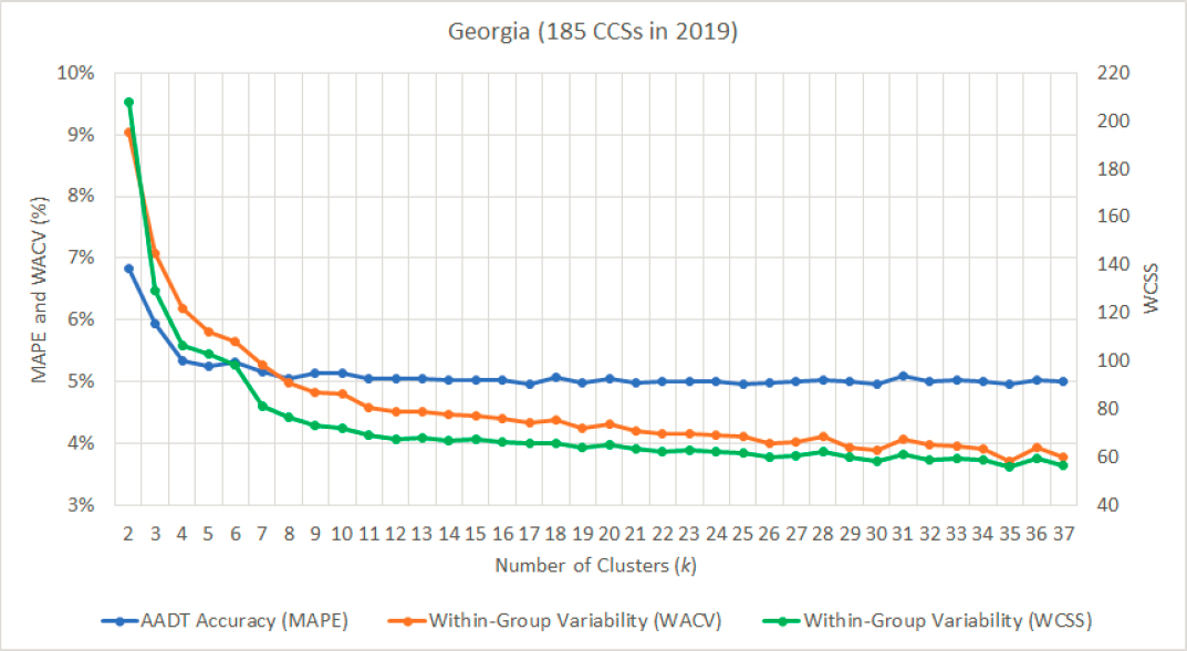
A common finding is that both the WCSS and the WACV continue to decrease even after the MAPE starts to plateau. For instance, in Figure 25, the MAPE stabilizes after creating four (k = 4) clusters, but the WACV and the WCSS continue to decrease at a relatively high rate until k = 11, after which their reduction rate significantly drops. Figure 26 shows a similar graph developed using 2015 data from 63 CCSs in Iowa.

In this example, no improvement in AADT accuracy is gained after creating more than three clusters despite the fact that the within-group variability continues to decrease until the maximum number (max k = 12) of clusters is reached. The WCSS and the WACV follow the same trend. The advantage of the WACV over the WCSS is that the former is expressed as a percentage, similar to the MAPE, making the visualization and interpretation of the results easier.
M13—New Inputs in Cluster Analysis
In M13, 21 sets of independent variables were separately used to perform clustering multiple times. Each time a different number of clusters (k∈[2, n/5]) was produced for each state and year. Each set was initially used to create two clusters (k = 2) per state and year. Then, clustering was re-run by increasing the number of clusters by one (k = 2+1 = 3). This repetitive process was performed multiple times for each state and year until the maximum k (=n/5) was reached, as explained in M10.
After all clusters were created, the LOO approach was used to validate the performance of each set of inputs. Figure 27 shows the AADT accuracy (MAPEs) associated with each set of variables. The MAPEs are aggregated across all 135 state-years. The three colored bars shown for each set of inputs correspond to the MAPEs obtained from the development and validation of 3, 9, and 15 clusters, respectively. The sets of inputs are sorted in ascending order from the lowest to the highest MAPE calculated from the validation of three clusters. For comparison purposes, the figure also shows the three MAPEs obtained from M10, which involved developing clusters using the 84 MDWFs of each CCS.

The main findings from Figure 27 are as follows:
- The three sets of variables that yield the lowest MAPEs are the 84 MDWFs (M10), the 12 MFs, and the 365 DFs, respectively.
- The 12 MFs and the 365 DFs result in lower errors compared to the corresponding 12 monthly volumes and 365 daily volumes.
- Not surprisingly, the more clusters that are created, the higher the AADT accuracy; however, in most cases the difference in MAPEs between nine and 15 clusters is small, as explained previously. One exception is the census density variables (i.e., employment, household unit, population, worker density), whose errors remain stable at approximately 9.0 percent regardless of how many clusters are created. This indicates that the census variables cannot effectively capture the variability in temporal traffic patterns.
- The four sets of HFs that include 2,016 one-hour, 1,008 two-hour, 672 three-hour, and 336 six-hour factors, respectively, produce similar results.
- Combining any variable with the geographical coordinates of the CCSs produces slightly higher errors than using the variable alone, but the produced clusters tend to contain sites that are geographically closer.
- Although not shown in Figure 27, the results revealed that categorical variables like FC can be used either as a continuous or categorical variable. In both cases, it results in the same level of accuracy as M2, which involved manually grouping CCSs by FC.
M14—Assignment of SDCs to Clusters Using DTs
In M14, six DTs were developed for each state and year using six assignment attributes respectively (Table 28). Each DT was applied to (n/5−1) sets of clusters, which were separately created using 84 MDWFs (M10), 2,016 HFs (M13), and 12 MFs (M13). In the interest of brevity and considering the large amount of results generated in M14, a judicious selection of outcomes is presented herein. The showcased results are representative and collectively convey key findings from the analysis. Table 28 shows the average success rate of the six DTs applied to 3, 6, 9, and 15 clusters, which were created using the three clustering inputs stated above.
Table 28. Success Rate of DTs for Different Assignment Inputs and Different Types of Clusters.

The main findings from Table 28 are as follows:
- The success rate tends to decrease as the number of clusters increases. This can be better understood by considering the fact that the statistical probability of randomly assigning a count to the correct cluster decreases as the number of clusters increases. For example, the probability of correctly assigning a count to one of three clusters is 33.3 percent, but the probability is reduced to 11.1 percent when the count needs to be assigned to one out of nine clusters.
- The success rates of all DTs are higher than the corresponding statistical probability of randomly assigning a count to the correct cluster. For example, as explained above, in the case of three clusters, the probability of randomly assigning a count to the correct cluster is 33.3 percent, yet all six DTs have a success rate of 56.8 percent or higher. Likewise, in the case of nine clusters, the probability of a correct assignment is 11.1 percent, yet all six DTs have a success rate of 19.1 percent or higher.
- Among the six sets of DT inputs, the first set, containing 8,760 HFs, consistently yields the highest success rates across all types of clusters presented in the table. The second most effective set of DT inputs is the one that contains 2,016 HFs. The success rates exhibit a decreasing trend from the left to the right side of the table.
- A comparison of the results among the three clustering inputs shown in the second column reveals that the highest success rates are obtained for the clusters created using the 2,016
- HFs. This can likely be attributed to the fact that the 2,016 HFs have more similarities with the DT inputs since they both capture some of the traffic variability within a day. In contrast, the 84 MDWFs and the 12 MFs result in lower success rates because they are more dissimilar to the DT inputs since they do not capture any of the hourly or daily traffic variability, which exists within the DT inputs. However, high assignment success rates do not necessarily correspond to high AADT accuracy, as explained below.
Table 29 shows the MAPEs obtained for the six DTs applied to different types of clusters.
Table 29. AADT Accuracy (MAPE) of DTs for Different Assignment Inputs and Types of Clusters.

The main findings from Table 29 are as follows:
- As more clusters are created, the AADT accuracy tends to remain stable or marginally decrease. This can be better understood by considering two facts. As shown in M10, when the cluster membership of the counts is known, and therefore the success rate is 100 percent, the MAPEs tend to remain stable after a certain critical number of clusters. However, as explained above, in M14 the success rate is not 100 percent and continues to decrease as the number of clusters increases. As a result, the MAPEs shown in Table 29 tend to remain stable or slightly increase as more clusters are created.
- Among the six sets of DT inputs, the first set that contains 8,760 HFs results in the lowest MAPEs. In general, the MAPEs slightly decrease from the left to the right side of the table.
- The three clustering inputs shown in the second column yield similar MAPEs. In other words, the AADT accuracy is affected to a greater extent by the DT inputs than the clustering inputs provided that the latter capture temporal (e.g., seasonal, monthly, etc.) traffic patterns that are necessary to effectively annualize SDCs.
M15—Assignment of SDCs to Clusters Using SVMs
Similar to M14, six SVMs were developed in M15 for each state and year using the same six assignment attributes respectively (Table 30). Each SVM was applied to (n/5−1) sets of clusters, which were separately created using 84 MDWFs (M10), 2,016 HFs (M13), and 12 MFs
(M13). Table 30 shows the average success rate of the six SVMs applied to 3, 6, 9, and 15 clusters, which were created using the three clustering inputs stated above.
Table 30. Success Rate of SVMs for Different Assignment Inputs and Different Types of Clusters.
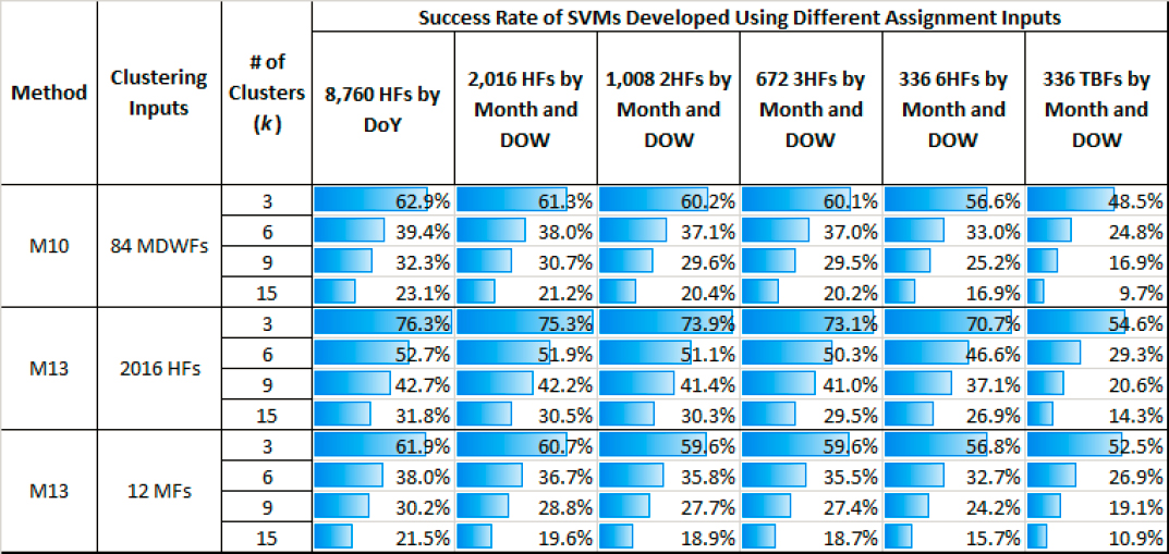
In general, the SVMs produced better results than the DTs, but the main findings and trends observed in Table 30 are similar to those in Table 28:
- The success rates tend to decrease as the number of clusters increases.
- The success rates for the majority of the SVMs are higher than those of the DTs. This can likely be attributed to SVMs’ superior ability to model complex data relationships more effectively than the DTs, which have a simpler structure.
- The success rates exhibit a decreasing trend from the left to the right side of the table. Among the six sets of assignment inputs, the first set, containing 8,760 HFs, consistently yields the highest success rates across all types of clusters presented in the table. The second most effective set of SVM inputs is the one that contains 2,016 HFs.
- A comparison of the results among the three clustering inputs reveals that the highest success rates are obtained for the clusters created using the 2,016 HFs, followed by the 84 MDWFs and then the 12 MFs.
Table 31 shows the MAPEs obtained for the six SVMs applied to different types of clusters.
Table 31. AADT Accuracy (MAPE) of SVMs for Different Assignment Inputs and Different Types of Clusters.
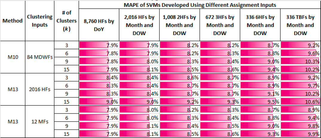
The main findings from Table 31 are as follows:
- As more clusters are created, the AADT accuracy tends to remain stable or marginally decrease. This is likely due to the reduction in the success rate as the number of clusters increases, coupled with the fact that after a certain critical point, the MAPEs tend to remain stable, as shown in M10.
- Among the six sets of SVM inputs, the first set that contains 8,760 HFs results in the lowest MAPEs. In general, the MAPEs slightly decrease from the left to the right side of the table.
- Among the three clustering inputs shown in the second column, the 84 MDWFs yield slightly lower MAPEs than the 12 MFs, followed by the 2,016 HFs. Despite the 2,016 HFs having the highest success rates (Table 30), they resulted in slightly higher errors than the other two sets of clustering inputs in most cases.
- In general, the AADT accuracy is affected to a greater extent by the SVM inputs than the clustering inputs as long as the latter account for seasonal traffic patterns.
- The SVMs (M15) produce more accurate AADT estimates than the DTs (Table 29).
NEW METHODS
M16—Assignment of Counts to Individual CCSs Using DTs
This method involved using DTs to assign sample counts extracted from a single CCS to another CCS within the same FC. Six DTs were developed for each state and year using the same six assignment attributes that were also used in M14 and M15. For comparison purposes, Figure 28 shows the AADT estimation errors (MAPE) of the six DTs developed in M16, as well as those obtained from the SVMs employed in M17, and the errors generated from the best performing DT and SVM from M14 and M15, respectively.
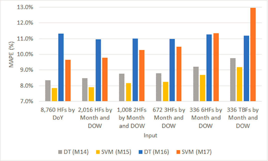
The main findings from Figure 28 are as follows:
- A comparison of the errors among all four methods shows that assigning counts to clusters (M14 and M15) results in more accurate AADTs than assigning them to individual CCSs (M16 and M17). This difference likely stems from the fact that methods M16 and M17 base their assignments solely on similarities in hourly traffic patterns between the count location and the CCS location on the specific day of the count. In other words, M16 and M17 do not consider any similarities in monthly or seasonal patterns between the two locations (count vs. CCS). As a consequence, M16 and M17 assign a count to the CCS with the most similar hourly traffic patterns on the specific day of the count, yet there is no assurance that the monthly or seasonal patterns at the CCS location are similar to those at the count location; however, the factoring process involves using monthly day-of-week factors—not hourly factors. Conversely, in M14 and M15, each cluster exhibits similar monthly and day-of-week traffic profiles. This characteristic proves to be more effective in the factoring process than not accounting for monthly and day-of-week patterns at all.
- Most SVMs in M17 result in more accurate AADTs than the DTs in M16. This can likely be attributed to SVMs’ superior ability to model complex data relationships more effectively than the DTs, which have a simpler structure.
- All six DTs in M16 yield similar-in-range MAPEs, despite the fact that they are statistically different at the 95 percent confidence level.
- The MAPEs of the six SVMs in M17 follow an increasing trend from the left to the right side of the table. The best performing set of SVM inputs is the one that contains 8,760 HFs.
M17—Assignment of Counts to Individual CCSs Using SVMs
The results from M17 are presented in the previous section.
M18—Annualization of SDCs Using Probe-Based Factors for Total Traffic
In M18, sample counts were annualized using segment-specific adjustment factors developed from raw probe count data that were provided by three vendors. Table 32 shows the average penetration rates of the three probe datasets and the correlations between the four probe-based adjustment factors and the corresponding actual adjustment factors calculated from CCS data.
Table 32. Penetration Rate of Raw Probe Data and Correlations of Probe-Based versus Actual Adjustment Factors (M18).
| Vendor (State) | Year | # CCS-Years | Avg. Penetration Rate | Correlations of Probe-Based vs. Actual Adjustment Factors | |||
|---|---|---|---|---|---|---|---|
| 7 Day of Week | 12 Monthly | 84 Monthly Day of Week | 365 Daily | ||||
| Vendor A (TX) | 2021–2022 | 209 | 5.83% | 0.817 | 0.788 | 0.795 | 0.844 |
| Vendor B (OH) | 4/1/2021–3/31/2022 | 46 | 0.39% | 0.549 | 0.509 | 0.399 | 0.311 |
| Vendor C (MN) | 2017–2019, 2021 | 97 | 2.86% | N/A | 0.325 | N/A | N/A |
The average penetration rates vary significantly from 0.39 percent to 5.83 percent, primarily because each vendor obtains its probe data from different sources. The highest penetration rate was determined for Vendor A, which obtains connected vehicle data from several original equipment manufacturers (OEMs). The data of the other two vendors primarily include location-based services data generated or collected from smartphones or other probe and GPS devices. Raw probe trip counts may vary for reasons unrelated to traffic volumes, such as a change in the penetration rate of roadway users using location-based services or connected vehicles or a change in the vendor’s data sources. Vendor A exhibits the highest correlation for daily factors (0.844), followed by day-of-week (0.817) and monthly day-of-week (0.795) factors. Conversely, Vendor B demonstrates the highest correlation for day-of-week factors (0.549), followed by monthly (0.509) and monthly day-of-week (0.399) factors. This trend suggests a sample size effect since the average penetration rate for Vendor B is low, at 0.39 percent. For instance, the calculation of each annual day-of-week factor includes up to 52 or 53 ADTs per day of week, and as a result, it averages out fluctuations occurring at the daily level. The probe data of Vendor C have a higher penetration rate (2.86 percent) than those of Vendor B, yet the correlation for the 12 MFs is lower. This discrepancy arises mainly because the probe counts of Vendor C are rounded up to the nearest thousandth, affecting the monthly patterns within a year.
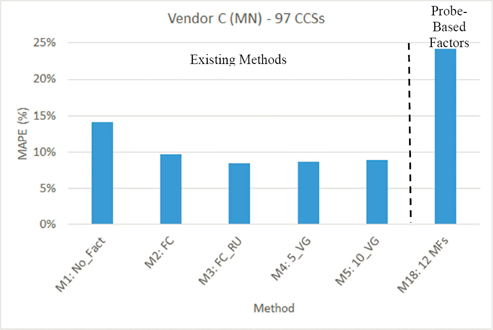
Figure 29 shows the MAPEs of AADT estimates derived from weekday (Monday–Friday) sample counts annualized using the existing methods (M1–M5) and the probe-based adjustment factors developed in M18 for Texas (Vendor A). Likewise, Figure 30 and Figure 31 show the MAPEs estimated using probe data from Vendor B (OH) and Vendor C (MN), respectively. For each state, all existing and probe-based methods were applied and validated using the same CCS-years for which probe data were obtained to ensure a fair comparison.

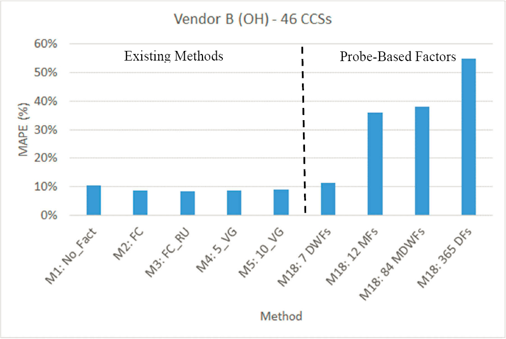
Note that the MAPE values, and hence the range of the y axis (MAPE), differ significantly among the three graphs. Figure 29 (Vendor A, TX) shows that among the four sets of probe-based factors, the seven annual day-of-week factors performed better than the other three sets. The second most effective set of probe-based factors was the one containing 84 MDWFs, followed by the set of 365 DFs. It is worth noting that the seven day-of-week factors resulted in the same MAPE (8.0 percent) as M2 (FC_RU). The other four existing methods (M1, M2, M4, M5) produced less accurate AADT estimates with errors ranging between 8.4 percent (M2) and 10.6 percent (M1).
In the case of Vendor B (Figure 30), the seven annual day-of-week probe-based factors performed significantly better (MAPE = 11.3 percent) than the other three sets. This outcome aligns with Vendor B’s day-of-week factors, which also exhibited the highest correlation with the actual adjustment factors, as shown in Table 32. However, the probe-based factors (M18) resulted in higher errors compared to those obtained from the five existing methods (8.5–10.6 percent). This suggests that as the correlation between the probe factors and the actual factors decreases, the AADT accuracy of counts factored using probe-based factors is expected to decrease as well. This finding holds true in Figure 31 (Vendor C, MN), which shows that the 12 monthly probe factors that have a weak correlation (0.325) with actual adjustment factors yielded significantly higher errors (MAPE = 24.2 percent) than all five existing methods, M1–M5. In general, a higher penetration rate typically leads to an increased correlation between probe and actual factors, resulting in greater AADT accuracy for counts factored using probe factors.
Table 33 shows various performance metrics aggregated by FC for the seven annual day-of-week factors, which is the best performing set of probe-based factors, developed using Vendor A’s raw probe data from Texas. The table shows the sample size, penetration rates,
correlations, absolute difference, APE, and PE percentiles aggregated by FC. The absolute difference, APE, and PE percentiles are based on factored weekday counts, from Monday to Friday.
Table 33. Performance Metrics Aggregated by FC for the Probe Data of Vendor A and the Seven Annual Day-of-Week Probe-Based Factors Validated in Texas.
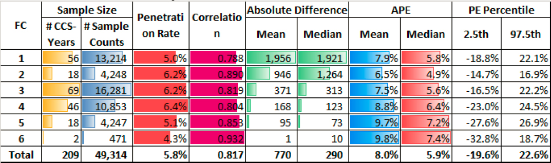
The main findings from Table 33 are as follows:
- The penetration rates tend to decrease from higher to lower FCs; however, the sample size in FC5 and FC6 is small and may lead to inconclusive results.
- Despite the penetration rates following this decreasing tend described above, the correlations follow the opposite increasing trend as one moves from higher to lower FCs. A larger sample size is needed, though, to draw more robust conclusions.
- The absolute difference between the estimated and actual AADTs decreases from higher to lower FCs, primarily because the traffic volumes also tend to decrease on lower FCs.
- The MAPE and the median APE exhibit similar trends. They slightly increase in the lower FCs, but this is expected because both metrics tend to increase as the volumes decrease.
- No unusual trends are observed in the 2.5th and the 97.5th percentile PE values.
Table 34 further disaggregates the results by FC_RU.
Table 34. Performance Metrics Aggregated by FC_RU for the Probe Data of Vendor A and the Seven Annual Day-of-Week Probe-Based Factors Validated in Texas.
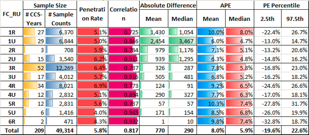
The main findings from Table 34 are as follows:
- Within each FC, the correlations on urban roads are consistently higher than those on rural roads, even though the penetration rates on 3R, 4R, and 5R are higher than the penetration rates on 3U, 4U, and 5U.
- Likewise, within each FC, the MAPEs and median APEs on urban roads are consistently smaller than those on rural roads, likely due to the higher correlations on urban roads, as described above.
- The absolute differences between the estimated and actual AADTs are higher for urban roads than rural roads, likely because the AADTs on urban roads are also higher than those on rural roads.
- The difference between the 97.5th and the 2.5th PE percentiles captures the spread or range of errors of 95 percent of the CCSs. A larger difference indicates a greater spread or dispersion of the errors, whereas a smaller difference suggests that most of the errors are concentrated within a narrower range. In all cases, the PEs of rural roads are more widely spread than those of urban roads.
M19—Annualization of SDCs Using Probe-Based Factors for Truck Traffic
In M19, the availability of Vendor C’s probe truck data at monthly aggregations only permitted the calculation of 12 MFs. Table 35 shows the average penetration rates of probe data for medium- and heavy-duty vehicles. The table also shows the correlations between the 12 monthly probe-based factors and the corresponding actual adjustment factors calculated from CCS vehicle classification data.
Table 35. Penetration Rates and Correlations of Probe-Based versus Actual Adjustment Factors (M19).
| Vendor (State) | Year | # CCS-Years | Vehicle Group | Avg. Penetration Rate | Correlation of Probe vs. Actual 12 Monthly Adj. Factors | MAPE |
|---|---|---|---|---|---|---|
| Vendor C (MN) | 2017–2019, 2021 | 44 | Medium-Duty Vehicles | 27.7% | 0.312 | 42.6% |
| Heavy-Duty Vehicles | 28.6% | 0.327 | 42.8% |
In general, the penetration rates are high and in the same range for both medium-duty (27.7 percent) and heavy-duty trucks (28.6 percent). The high penetration rates are likely a data artifact because, as explained previously, Vendor C rounds raw probe trip counts to the nearest 1,000. This rounding leads to weak correlations (0.312 for medium-duty vehicles and 0.327 for heavy-duty trucks) and introduces significant AADT estimation errors (42.6–42.8 percent), as shown in the last column of Table 35.
Not surprisingly, the MAPEs for the two truck class groups are significantly worse than those obtained from the use of factors developed for all vehicles (M18, see Figure 31). The rounding of raw probe trip counts partially explains the poor performance of M19 since the rounding error is proportionally larger at lower trip counts. However, AADT estimates for a subset of vehicle classes would be expected to have higher errors than those for all vehicles due to the smaller sample size of these subsets.


