Developing a Guide for Incorporating Uncertainty into Long-Range Transportation Planning (2026)
Chapter: Appendix A: Foundational Research: Uncertainty Drivers, Data, and Methods
Contents
2. Uncertainty in Decision-Making
Effective Planning Practices: Historical Overview and Industry Practice
Characteristics of Effective Frameworks and Methods
Usage of Planning Frameworks and Methods in Transportation
Managing Deep Uncertainty: Joining Qualitative and Quantitative Approaches
3. Data and Methods to Assess Uncertainty and Its Impacts
Summary of Data, Methods, and Tools
Specific Data, Methods, and Tools
4. Regulatory Context and Requirements
Long-Range Transportation Plan (State DOT)
Statewide Freight Plan (State DOT)
Transportation Asset Management Plans
Congestion Mitigation and Air Quality Improvement Program
Statewide Transportation Improvement Program
Metropolitan Transportation Plan
Transportation Improvement Program
Transportation Performance Management (TPM)
Report Overview
This appendix provides an overview of the foundational research that informed the creation of the guide, NCHRP Research Report 1168: Incorporating Uncertainty into Long-Range Transportation Planning: A Guide, meant to help transportation agencies better incorporate uncertainty into their long-range planning efforts. This appendix is organized into four chapters:
- Sources of Uncertainty contains an overview of a range of types of uncertainty that influence state DOTs and MPOs in their ability to carry out their missions and adhere to their long-range plans or investment programs
- Uncertainty in Decision-Making provides an overview of decision-making frameworks and processes used historically and at present to understand and manage uncertainty
- Data and Methods to Assess Uncertainty and Its Impacts addresses data, methods, and tools that are widely available to transportation agencies to address the effects of uncertainty
- Regulator Context and Requirements describes where transportation agencies, primarily state departments of transportation (DOTs) and metropolitan planning organizations (MPOs), must consider and incorporate uncertainty or risk in their required planning documents and highlights selected opportunities for additional consideration beyond requirements.
1. Sources of Uncertainty
This section contains an overview of a range of types of uncertainty that influence state DOTs and MPOs in their ability to carry out their missions and adhere to their long-range plans or investment programs. While the details vary by subject, the general approach of this section is for each source of uncertainty to: (a) provide an overview of the concept including any recent dynamics, (b) describe the factors that contribute to uncertainty in this area, and (c) describe implications for transportation and transportation planning. Because sources of uncertainty are by their nature dynamic, this section focuses on explaining why any given source is important and potentially impactful and on providing enough information and background to support someone who wishes to dig more deeply into the issue. It is not designed to be comprehensive or complete in terms of resources, as any such attempt would quickly be rendered out-of-date.
This report groups sources of uncertainty into four main categories and identifies specific sources of uncertainty in each category as shown in Figure 1. While this report largely discusses each of these sources of uncertainty independent of one another, it should be noted that the transportation system is complex and that the identified sources of uncertainty overlap both within and across the four categories identified. As planners consult additional resources to better understand how a source of uncertainty may impact their work, they should also consider the relationship with the other sources of uncertainty identified.

Technology and Behavior
This section describes sources of uncertainty affecting transportation agencies in the realms of technology and behavior. While different in many ways, technology can shape behavior and vice versa in ways that change the realm of what’s likely or possible over time.
Vehicle Automation and Related Technology
The evolving capabilities of vehicle automation and related technologies are saving lives and making roads safer. While driver assistance technologies have already hit the market, industry practitioners investigating cutting edge research and development are determined to make fully autonomous vehicles a reality too.
NHTSA defines the levels of vehicle automation as ranging from Level 0 to Level 5. In Levels 0-2, humans maintain full control over the vehicle but are supported by technologies that partially automate the driving experience (NHTSA, 2022). From Levels 3-5, driving is fully automated and requires little to no human control. Figure 2 lists the role of the human driver in each level and supporting features required within a vehicle to achieve the desired level of autonomy.
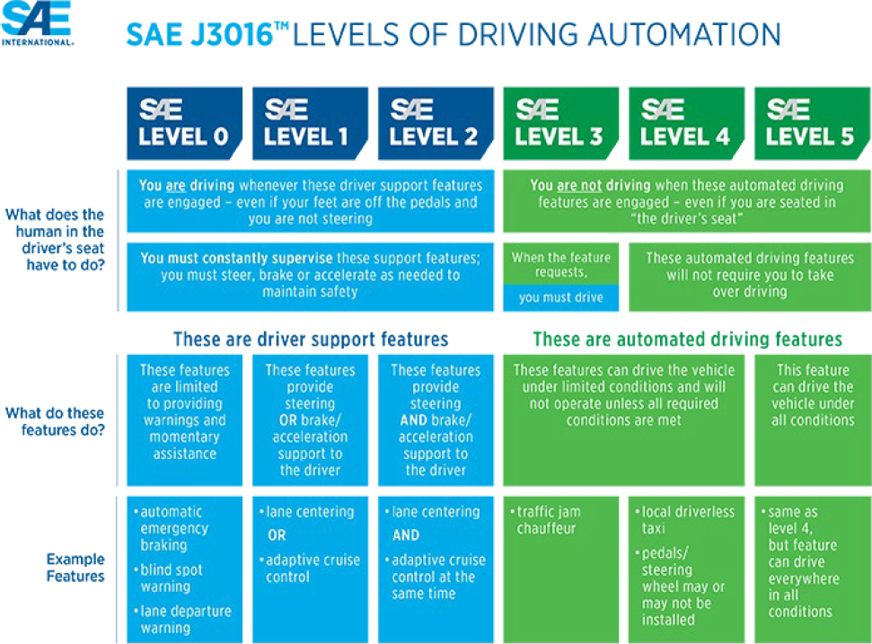
Source: SAE International
The race to commercialize Autonomous Vehicles (AVs) could mean multiple things for transportation planning. AV technology includes different components with each having its own impact on overall user behavior and the built environment. Some widely discussed benefits of AVs include increased mobility for nondrivers (including older adults, young people, some people with disabilities, and other people without a driver’s license) and an overall reduction in crashes that cost billions each year (NHTSA, 2022). AVs may also change people’s behavior by reducing the disutility of time spent in vehicles (Nair et al., 2018) and could reduce labor costs associated transportation service operations.
Research highlights the potential for changing land use patterns, with potentially conflicting dynamics. For example, if automation is accompanied by shared use, the need for parking spaces is likely to decrease (Zmud et al., 2016). Similarly, housing shortages could decrease as well if parking spaces are repurposed for houses. However, AVs could also increase suburban sprawl as the disutility of travel is decreased (Zmud et al., 2018). Impacts on energy consumption and emissions will depend on the resulting mix of land use changes, travel patterns, and the degree of electrification and fuel efficiency of AVs.
Zmud et al. (2018) summarizes a range of uncertainties that should be recognized in planning for autonomous vehicles, including uncertainty in:
- Adoption timelines
- Safety benefits and risks, including issues of cybersecurity
- Congestion impacts, including flow efficiency, as well as impacts on induced demand and vehicle occupancy through the evolution of fleet sharing versus private ownership
- Land development
The high degree of variability in outcomes based on different factors related to AVs is illustrated in Figure 3.
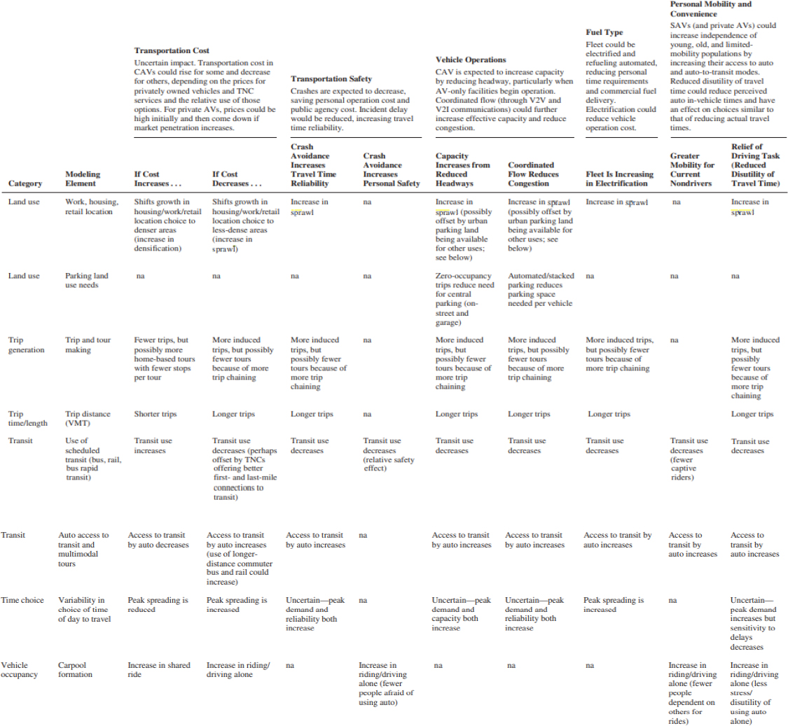
Source: d et al. (2018)
From a transportation performance perspective, one of the key considerations is the degree to which AVs could increase the effective capacity of roadways by allowing vehicles to follow each other more closely, as well as the degree to which this is less true in mixed conventional and autonomous traffic. Generation of additional zero occupancy vehicle trips (i.e., between dropping one passenger off and picking up another or between a drop-off and a parking location) is another topic with a large potential impact on overall traffic levels. Researchers and engineers are actively developing and testing new methods to represent these dynamics, particularly within travel demand models (Zmud et al., 2018; Saeid et al., 2020; VDOT, 2020; Nair et al., 2018). These
modeling techniques have been incorporated into scenario planning exercises to explore a range of impacts (Michigan DOT, 2021; NYSDOT, 2020).
While the industry is focused on getting the technology right, it is also pertinent for transportation authorities to understand the impact of AVs on design requirements for the built environment. AVs navigate infrastructure through perception sensors and LIDAR technology. Perception is negatively impacted by road sign non-uniformity or disorientation and performs much better when signs and pavement markings have high reflectivity and contrast (Booz Allen Hamilton, 2020). When considering a future shaped by AVs, transportation agencies therefore need to consider not only how system performance will be impacted, but also how transportation agency actions can either facilitate or hinder implementation.
Responding to the scope and scale of this issue, as well as its considerable ongoing uncertainty, the National Cooperative Highway Research Program has sponsored an entire program of research (NCHRP 20-102) aimed at understanding and managing the “Impacts of Connected Vehicles and Automated Vehicles on State and Local Transportation Agencies.”
Vehicle Electrification
The motor vehicle market’s composition is changing with regards to those that are fossil-fueled Internal Combustion Engine (ICE) vehicles and those that are Zero Emission Vehicles (ZEVs). The timing and nature of changes remain uncertain, with possible implications for infrastructure and planning. ZEVs, as defined by the California Air Resources Board, include Battery Electric Vehicles (BEVs), Plug-In Hybrid Electric Vehicles (PHEVs), and Fuel Cell Electric Vehicles (FCEVs). Factors behind this transition include technological advances, adoption of clean energy regulation, and community priorities aimed at reducing the negative environmental externalities of transportation.
Policy and Regulatory Context.
In 2022, the state of California updated its motor vehicle emissions regulations with the adoption of the Advanced Clean Cars II (ACC II) regulations. These regulations require that an increasing percentage of light-duty vehicles sold in the state be zero-emission vehicles (ZEVs), with a goal that by 2035 all new passenger cars, trucks, and SUVs sold in the state will be ZEVs. Other states have also adopted all or part of California’s low-emission and ZEV regulations (California Air Resources Board, 2025). California has also adopted the Advanced Clean Trucks (ACT) regulation with the goal of similarly mandating ZEV sales share targets and accelerating deployment of zero-emission trucks (California Air Resources Board, 2021). Other states have or are considering adopting the ACT regulations. Regulatory requirements mandating ZEV sales are helping to drive the market and create economies of scale that lower the overall costs of electrification (NESCAUM, 2022).
At the federal level, $5 billion dollars in funding through the Bipartisan Infrastructure Law for states was allocated to build out charging infrastructure (The White House, 2021). The Bipartisan Infrastructure Law (BIL) established the $5 billion National Electric Vehicle Infrastructure (NEVI)
Formula Program. To access this funding, each State DOT was required annually to develop an EV Infrastructure Deployment Plan (FHWA, 2022).
Resources, Forecasts, and Sources of Uncertainty.
Electric vehicle sales and the outlook for fleet transition is a closely tracked and forecasted topic. For example, BloombergNEF (BNEF) publishes an annual Electric Vehicle Outlook (BNEF, 2022) and EVAdoption provides EV forecast data (EVAdoption, 2022). In the public sector, the U.S. Department of Energy’s (USDOE’s) Clean Cities Coalition Network provides a centralized repository of resources (USDOE, n.d. a) and USDOE’s Alternative Fuels Data Center provides a wealth of data on vehicle and infrastructure trends (USDOE n.d. b). While recent trends and near-term forecasts indicate a rapid acceleration of EV deployment, the longer-term outlook is necessarily subject to sources of uncertainty including economic trends, changes in battery prices, policies and regulations, fleet turnover, charging infrastructure deployment, consumer preferences, supply chain constraints, gas prices, and changes in EV technology and range (BNEF, 2022). One particularly uncertain dynamic is the likely evolution of technology for short-haul versus long-haul trucking, with electricity potentially emerging as the fuel of choice for shorter trips but hydrogen potentially offering a better solution for long-haul trips (NREL, 2022).
Impacts on Transportation Planning.
The need to plan for charging infrastructure is the key transportation infrastructure impact of vehicle electrification. EVs will also have major impacts on transportation-related performance in the areas of health, air quality, and environment through the reduction of emissions. Transportation agencies can leverage resources such as the EPA’s MOtor Vehicle Emission Simulator (MOVES) to forecast vehicle emissions (EPA, 2022). EVs may also have impacts on safety, pavement management, bridge management, and other performance areas as current battery technologies are considerably heavier than ICE vehicles (NCST, 2021). This can affect performance forecasting, project and plan impact assessments, and the setting and monitoring of performance targets.
EVs will require new/enhanced coordination between transportation agencies, utilities, and state energy offices (FHWA, 2022). EVs will additionally have operational and cost implications for agency fleets. Transit agencies and operational and maintenance vehicles owned by states and localities have opportunities for fleet transition. This will require planning to reflect shifts in fuel/electricity budgets, likely savings in operations and maintenance expenditures for EVs (USDOE, 2022), and changes in workforce needs (San Diego Workforce Partnership, 2019).
Policymakers and planners are also concerned with how best to include all communities in realizing the benefits of vehicle electrification technology (Wazowicz, 2021). This demands a focus on who can share in the benefits of personal vehicle electrification, community fleet electrification, and reduced emissions, while also considering who might bear new burdens or be left behind by a transition.
Finally, electrification has major impacts on fuel tax revenues, the primary transportation funding instrument nationally and for all states.
Household and Firm Location Choice
Both household and firm location choices are dynamic and subject to change over time, influencing patterns of transportation demands. While uncertain over the long-term, large-scale changes in location choices are typically slow to manifest and not generally subject to sudden shocks. As such, they can be tracked and monitored over time but are still uncertain at the timescale of long-range transportation plans.
Household Location Choices - Changing Dynamics and Uncertainties.
Household location preferences are influenced by a wide range of factors including transportation accessibility, price, household characteristics, environmental quality, and lifestyle preferences. These are often addressed through economic and forecasting methods, including hedonic price and land use modeling. For example, CommunityViz is one tool used in planning practice to allocate growth spatially across a region using an analysis of defined suitability parameters that drive the attractiveness of any given parcel to a particular land use (Triangle J COG, 2020).
While many of the factors that drive location choices are relatively stable, there are instances of changing preferences that introduce uncertainty or may require adaptation of expectations and forecasting methods over time. For example, researchers have investigated the degree to which younger generations (e.g., Millennials) show greater interest in denser more walkable urban environments relative to prior cohorts (Evans, 2017; National Association of Realtors, 2015)—with mixed findings on whether observed variations are true differences in preferences or tied to other factors like delayed household formation (Bialik and Fry, 2019). On the other hand, data collected since COVID-19 pandemic identifies shifts towards suburban living (Steutville, 2021). Vehicle automation raises questions about whether the technology will accelerate sprawl once people can use their time productively while driving (Guan et al., 2021). Given these dynamics, many agencies have recognized degree of urbanization as a significant source of uncertainty for transportation planning and chosen to explore implications of alternative growth patterns though scenario planning. For example, the Hampton Roads TPO developed scenarios focused around urban and suburban preferences in the context of planning major future infrastructure investments (HRTPO, n.d.).
Business Location Choices - Changing Dynamics and Uncertainties.
As with households, business location choices are influenced by many factors, including industry-specific needs. Changing preferences over time reflect changing technological and operational parameters. For example, researchers have investigated how the rise of knowledge industries increased emphasis on business colocation and chasing talent, resulting in urbanized preferences for certain sectors (APTA, 2013). Others are studying how the rise of high-cube and automated warehousing can decrease land requirements relative to traditional logistics operations resulting in new location choices (LVPC, n.d.). Other issues like supply chain restructuring, including offshoring and nearshoring dynamics, the weighing of system resilience against efficiency, and the emphasis on rapid fulfillment in e-commerce can also result in restructuring of business location dynamics (Brown, 2020; Caplice and Phadnis, 2013).
Impacts on and Strategies for Transportation Planning.
Strategies for understanding and managing long-term uncertainty around location preferences include:
- Location trend analysis, particularly by demographic or industry cohort
- Coordination with subject matter experts including economic development professionals, land use planners, and freight stakeholders (such as through freight advisory committees)
- Preference surveys such as those conducted in the real estate or site selection industries
- Reliance on tools and expertise like economic forecasting and land use models
- Scenario planning exercises
Micro and Shared Mobility
Data from the 2017 NHTS shows that more than one in five privately-operated vehicle trips in the United States are 1 mile or less, and advances in technology have begun to offer travelers a greater number of “micro” mobility options to easily travel short distances (FHWA, 2017). The FHWA defines micromobility as “as any small, low-speed, human- or electric-powered transportation device, including bicycles, scooters, electric-assist bicycles, electric scooters (e-scooters), and other small, lightweight, wheeled conveyances” (Price et al., 2021). While some traditional transportation modes, such as biking, fit within this definition, the rise in popularity of newer modes such as e-bikes and e-scooters has increased uncertainty for transportation planners. Greater use of micromobility vehicles will place a larger demand on infrastructure that has traditionally served cyclists (such as bike lanes and bike parking), though limited data on the rate of micromobility vehicle adoption makes it difficult for planners to determine how quickly such infrastructure should be expanded (USDOT, 2022). Further, the use of electric micromobility devices may necessitate charging infrastructure to serve e-bikes and e-scooters. The smaller size and travel radius of electric micromobility vehicles may allow users to charge their vehicles at their place of residence, though charging infrastructure at workplaces and public places may offer micromobility users the flexibility to take longer or more frequent trips (USDOT, 2023). While estimates of e-bike sales nearly doubled to 790,000 from 2020 to 2021, planning for charging infrastructure is complicated by limited information on the rate of electric micromobility use and a lack of standardized charging equipment for electric micromobility vehicles (USDOT BTS, 2022; USDOT, 2023).
Advances in technology have also changed traditional vehicle ownership models, allowing travelers to share transportation services and resources in new ways. The Federal Transit Administration broadly defines shared mobility as “transportation services that are shared among users,” and includes public transit, taxis and limos, bikesharing, scooter sharing, carsharing, and ridesharing, among other modes, in its definition of shared mobility (FTA, 2020). Shared mobility services offer travelers many of the benefits of private vehicle ownership without the commitment and cost of vehicle ownership. While shared mobility services are largely designed to utilize existing transportation infrastructure, they do have some unique infrastructure requirements, such as parking spaces for shared cars, docking stations or dedicated parking areas for shared bikes and scooters, or dedicated pickup areas for ridesharing services like Uber,
Lyft, or other Transportation Network Companies (TNCs). Researchers are actively investigating the rate at which shared mobility services might be adopted and replace traditional vehicle ownership models, creating uncertainty for transportation planners who must anticipate future infrastructure needs.
New shared mobility technologies have implications for public transit as well. “Microtransit” reimagines traditional public transit services so that transit vehicles do not run on fixed routes, but rather respond in real-time to the travel and schedule demands of riders (Shaheen et al., 2016). These services often rely on similar technologies to those seen in TNC services and have the potential to increase transportation accessibility for transit riders in rural, suburban, and urban areas. While microtransit services can be more expensive than traditional fixed-route services when used at a large-scale (Bardaka at al., 2020; NCDOT, 2023), the ability to offer targeted transit service to riders only when and where they need it can make microtransit a cost-effective solution in areas with low population density. Transportation agencies have piloted microtransit services as both a supplement to (LA Metro, n.d.) and replacement of traditional fixed-route transit services (NCDOT, 2023). Increased adoption of microtransit may disrupt traditional vehicle ownership models, compete with other micromobility modes for travel demand, and change traditional transit service models. Autonomous micromobility vehicles, though, may be able to offer microtransit services at a lower cost than those seen currently.
In addition to the uncertainty associated with micro and shared mobility’s unique infrastructure needs, these new mobility options create additional uncertainty for transportation planners since they have the potential to disrupt the existing transportation system. Micromobility devices may be able to replace short car trips and therefore ease congestion (Fan and Harper, 2022), while ridesharing TNCs may be creating additional congestion on existing roadways as drivers circle areas waiting for riders to call a vehicle (Roy et al., 2020). The degree to which micro and shared mobility may complement or substitute trips on other modes of transportation is also not yet well understood, since research on the topic is often challenged by limited data availability. In a review of the research that does exist, Wang et al. (2023) found that e-scooters may replace between 3 and 18% of public transit trips, though they are likely to replace car trips (between 5 and 45% of trips) or walking trips (between 5 and 77%) at a higher rate. Researchers have also found that micro and shared mobility options can increase accessibility to public transit (Liu and Miller, 2022), though it’s unclear how extensively travelers may use micro and shared mobility options to complete first and last mile connections to public transit.
Practitioners, researchers, and entrepreneurs have expressed an interested in integrating these new micromobility options into “Mobility as a Service” (MaaS) platforms. With several conceptualizations and few real-world examples, MaaS does not have a definition that has been universally adopted. It has generally been envisioned to be a means of offering users unified access to a variety of mobility platforms, often through a smartphone-based app. Researchers have conceived of multiple business models for MaaS, with the primary models being a pay-as-you-go format, where users pay for the transportation services they consume across modes in a single interface, and a subscription-based format, where users pay a monthly fee and are offered
a bundle of credits to use for rides across transportation services (Sochor et al., 2018). The implementation of MaaS is challenging since it requires partnerships between public and private entities, as well as partnerships between private businesses. The MaaS pilots that have been implemented have often been time-limited, small-scale, and not financially self-sustaining (Hammond, 2023; Mitropoulos et al., 2023). If implemented at a larger scale, MaaS has the potential to disrupt vehicle ownership models, change modal preferences, increase transportation accessibility, and allow for greater integration across modes. While the future of MaaS is uncertain, transportation planners can prepare for the uncertainty it creates by increasing the capacity of modes other than the personal automobile, tracking the evolution of payment technologies and integration efforts, and being open to partnerships with public and private entities that seek to provide streamlined access to mobility options.
Mode Choice
Like household and firm location choices, modal preferences also depend on a variety of factors and are subject to change over time. Travel modeling typically involves discrete choice methods calibrated using survey or other data on observed travel choices to understand the “revealed preferences” of travelers as a function of the attributes of available options (e.g., travel time, cost, reliability, etc.). Modeling tools and methods are updated on an ongoing basis, as supported by cycles of data collection. Choice model estimation can also incorporate data from “stated preference” surveys. This can be particularly helpful for new modal options on which current data does not exist.
There can be instances of change in latent modal preferences over and above what may be driven by changing demographics or transportation system characteristics. For example, a study using repeated cross-sectional travel diary data from people in the San Francisco Bay Area in 2000 and 2012 identified changes in modal preferences reflecting cultural shifts across generations as an underlying driver of decreases in private vehicle mode share. Had these preference changes not been a factor, other trends in the socioeconomic environment and transportation infrastructure would have indicated an increase in driving (Vij et al., 2017).
The above example points to the uncertainty in mode choice over longer time horizons. In practice, transportation agencies have managed this uncertainty by investing in data collection and modeling method updates on an ongoing basis. Technology is also making data collection on travel behavior easier and less burdensome, including GPS supported automated travel diaries (UC Davis and Caltrans, 2007) and the use of data from transit Automated Fare Card systems.
E-commerce
E-commerce, which includes any goods and services sold online, has grown steadily as a share of total retail sales since 2013 (Figure 4). Sales data from 2021-2022 suggest the spike in e-commerce sales during 2020 was temporary and is leveling off, and growth will likely continue along a long-term linear trendline. Nonetheless, pandemic-era changes to consumer, retailer, and logistics and delivery provider behavior remain. Broadly speaking, the literature addresses e-commerce issues related to curbside pickup, local delivery from retailers like grocery stores,
prepared food delivery from restaurants, non-Amazon online retail deliveries, and Amazon deliveries as segments of e-commerce activity.
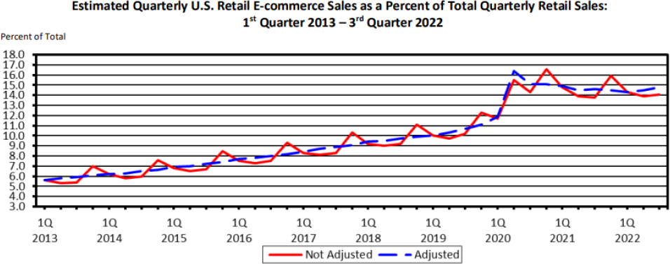
Source: U.S. Census Bureau Economic Indicators Division 2022.
Transportation planners should consider how e-commerce growth will strain urban freight distribution systems. The literature emphasizes that growing e-commerce sales exacerbate externalities associated with last-mile delivery, including traffic congestion, lack of parking, pollution, and noise in urban areas where population density is increasing (Viu-Roig and Alvarez-Palau, 2020). Planners’ ability to address these challenges may constrain or accelerate e-commerce growth in urban areas, as well as mitigate or amplify its negative effects on residents’ quality of life. This dynamic is one source of uncertainty in anticipating and managing the impacts of e-commerce.
Another source of uncertainty is the difficulty in forecasting the future evolution of e-commerce, given the many dimensions of the phenomenon. FHWA notes in a 2019 report that measuring and forecasting regional freight activity is difficult given that e-commerce blurs lines between personal and commercial freight, as well as its origins and destinations (FHWA, 2019). A dramatic uptick in e-commerce adoption during the COVID-19 pandemic exacerbated these measurement problems.
In studying the dramatic uptick in e-commerce activity, the North Jersey Transportation Planning Authority (NJTPA) found in 2020 that population, number of households, household income, and median age are strong predictors of changing e-commerce demand in a zip code—though age will likely be less relevant as adoption of e-commerce grows (NJTPA, 2020). These predictors are important because traditional commodity flow databases do not include last-mile delivery trips. One solution is to use population and household forecasts by zip code to forecast e-commerce demand, then adjust upward to estimate e-commerce’s growing market permeation (NJTPA, 2020).
The degree to which e-commerce results in substitutions between trip types (shopping versus home-delivery or consumer pickup) is another dynamic and evolving topic. During the COVID-19 pandemic, Jaller (2021) observed several key trends in consumer behavior in the Sacramento region, including (1) fewer in-store shopping trips; (2) larger in-store basket sizes; and (3) more frequent e-commerce purchases and new e-commerce users. Jaller also notes that higher e-commerce sales do not necessarily reduce consumer trips, since many consumers still use curbside or alternate location pickup for their orders. Viu-Roig and Alvarez-Palau (2020) found that alternate pickup locations like lockers and mobile depots help to reduce the negative externalities e-commerce creates in cities from direct home deliveries and is viewed favorably by consumers, logistics providers, and retailers.

Source: UC Davis 2020.
Rush service is another key driver of change to demand- and supply-side behavior in e-commerce. Figure 5 shows that high rush and time sensitive deliveries like grocery orders spend more emissions and VMT compared to deliveries with a wider time frame following the customer order (Jaller, 2020). This suggests rush delivery can be a major source of roadway congestion, as smaller vehicles deliver fewer goods in a shorter timeframe and cannot take advantage of economies of scale. NJTPA (2020) similarly notes that customization, rush delivery, and extended delivery hours drive consumer demand for e-commerce over brick-and-mortar retail.
Alho et al. (2021) found that new services like on-demand delivery, where individuals use personal cars to make local deliveries, have the potential to fulfill a significant amount of rush delivery demand while decreasing freight vehicle traffic and vehicle-miles-traveled. Additionally, delivery-on-demand services do not compromise the quality of similar ride-share services for passenger travel. Similarly, Viu-Roig and Alvarez-Palau (2020) found many urban planning experts advocate for cargo bicycle, automated, and public transport-based distribution systems to reduce the impact of last-mile delivery on cities. Evolving modal options require new modeling tools. For example, Simmobility is a simulation software that models changes to commodity contracts, logistics, and vehicle operation planning and parking decisions. This simulation ability is one way to understand the impacts of alternative freight distribution systems like on-demand delivery and cargo bicycles compared to the current state (Alho et al., 2020).
Implementation of new last-mile delivery systems will require infrastructure modifications, new regulatory frameworks, pilot programs, and new technology adoption to be an efficient alternative to traditional vehicle delivery (Viu-Roig and Alvarez-Palau, 2020). Public authorities play a key role as decision makers that can influence a modal shift in urban logistics.
There are many interconnected dynamics within the overall concept of e-commerce that are still evolving, including various forms of consumer purchase, delivery, and pickup. These various business models can either exacerbate or reduce the negative externalities of freight and last-mile delivery and may be influenced by the actions of both the public and private sectors. Both the long-term demand for and impact of e-commerce are difficult to forecast. As such, these factors require ongoing monitoring and attention by transportation agencies, as well as continued engagement between the public and private sectors.
Telework
The rate of individuals teleworking, or working from home, was increasing over time prior to the COVID-19 pandemic as seen in Figure 6, particularly in certain occupations, but was still relatively limited (RSG, 2021). However, between 2019 and 2021, and as a result of the public health crisis and associated stay-home guidelines, the number of people primarily working from home tripled from 5.7 percent to 17.9 percent (U.S. Census, 2022a).

Source: RSG 2021.
This major shift in the number of people working from home dramatically changed commuting behavior and decreased demand on the transportation system, particularly in peak periods. Over time, the relaxation of pandemic rules and guidelines, coupled with advances in vaccination, have led to a gradual, if uneven, return to work as well as other trip-making. Figure 7 shows how at the height of the pandemic, total passenger vehicle miles traveled (VMT) estimated based on INRIX
data declined to approximately 40 percent of benchmark levels (what would have been expected without a pandemic) but has since more than rebounded.

Source: BTS 2021.
There remains significant uncertainty around the extent to which high levels of telecommuting will endure as a phenomenon shaping demand on the transportation system. Factors that are likely to affect the long-term outlook for telecommuting include:
Limitations on the types of jobs that can be accomplished remotely.
Researchers from the University of Chicago estimated in 2020 that 37 percent American jobs could be done at home based on detailed occupational information, with the share ranging from approximately all jobs in computer and mathematical occupations to no ability to work from home in food preparation or cleaning and maintenance (Dingel and Neiman, 2020). This research was reinforced by observations during the pandemic of unequal access to telework. In a national survey, RSG found that black respondents and those with lower incomes were telecommuting at lower rates (RSG, 2020). Similarly, the Survey of Household Economics and Decisionmaking (SHED) highlighted how workers with more education and younger workers have been much more likely to work from home during the pandemic (Federal Reserve, 2021). The differential potential for telework has implications for various traveler cohorts in the future and for spatial patterns of demand as some types of employment centers are likely to be impacted more than others. The impact of telework is also not felt evenly across travel modes, as many transit users work in occupations that require in person presence (ATL, 2020).
The evolution in worker and employer preferences and part-time commuters.
While the pandemic pushed limits on the possibility of telework, the enduring power of this option depends on worker and employer preferences (or requirements). An RSG national survey found that people working from home as of 2021 would prefer in the future to do it 2.7 days per week and that these same respondents estimate that about two-thirds of their employers would be supportive of this
preference (RSG, 2021). Similarly, the US Census Pulse Survey from November 2-14, 2022, found that 14 percent of those responding to a question on whether anyone in their household worked from home in the last 7 days said yes for between 1 and 4 days, while 16 percent said yes for 5 days or more (U.S. Census, 2022b). Future planning will need to account for the likelihood of part-time commuters.
The scale of impact of commuting vis-à-vis other trip-making.
Regardless of the number of people working from home, there is not a one-to-one relationship between removed commuting trips and a decrease in demand and VMT on the system. In fact, He and Hu (2015) found in Chicago that telecommuting increases the total number of trips even though it decreases commute trips. Why this occurs or whether it is predictive for the future remains to be explored. Additionally, while there may be offsetting effects in terms of the number of trips, the destinations and lengths of trips may be very different. This dynamic is hinted at by data from 2022 that show an increase in trips less than one mile compared to 2019 (BTS, 2022).
Even in the absence of offsetting trips, commuting trips make up only 30 percent of all passenger miles traveled (BTS, 2018), which will mute the impact of telework on overall traffic.
In response to the above outlined uncertainties, State DOTs and MPOs are actively using surveys to monitor and understand trends in work-from-home behaviors and preferences, as well as developing and modeling scenarios to explore the impacts on travel demand and needs (Qian and Linscheid, 2022; ARC, 2021; TRB, 2021).
Safety (Technology and Behavior)
Road safety is a top priority for transportation stakeholders. Over the years we have seen improvements in overall traffic safety with significant contributions by relevant stakeholders to make roads safer. However, the 2020 crash fatalities report (during COVID-19) bucked trends as NHTSA reported the largest projected number of fatalities since 2007. This was particularly alarming because crash rates increased despite a 13.2 percent in vehicle miles traveled (VMT) (AASHTO, 2021). As transportation agencies continue to work towards reducing crashes and associated fatalities, injuries, and property damage, they are challenged to understand the underlying factors that drive safety outcomes, many of which have some aspect of uncertainty.
Forecasting and safety target setting.
State DOTs, in coordination with MPOs, report safety performance to FHWA annually and set targets and monitor trends through Highway Safety Improvement Program (HSIP) reports. Agencies face a number of challenges in collecting and forecasting safety data. This includes data quality issues, particularly for non-motorized incidents. Safety data collection also requires significant coordination between transportation agencies and law enforcement. With respect to forecasting to support target setting and performance monitoring, some agencies simply focus on trendlines, while others employ more complex statistical methods that seek to understand the influence of underlying factors. For example, Virginia DOT revised its target setting and forecasting approach in 2017 after an uptick in fatalities and serious injuries, building a “data-heavy regression model,” incorporating the variables shown in Table 1 (Grant et al., 2022). Many of these variables, though, are subject to
uncertainty. Moreover, the underlying relationships implied by such a modeling exercise can be altered by emerging technologies and behavioral shifts over time.
Table 1: Independent Variables Employed by VDOT to Forecast Safety Performance
| Category | Independent Variables |
|---|---|
| Socioeconomic Data |
|
| Travel and Behavioral |
|
| Transportation Spending |
|
| Weather |
|
Source: Grant et al., 2022.
Accounting for Emerging Technologies.
New transportation technologies present unique challenges as well as solutions to road safety issues. In 2020, 38,824 people lost their lives in motor vehicle crashes (NHTSA, 2022). Driver error is believed to be the primary reason for more than 90% of the crashes (FHWA, 2021), which makes the safety promise of automation and driver assistance systems quite strong. Technologies that are already being implemented in commercially sold vehicles include collision warnings, lane departure warnings, automatic braking systems, lane centering assistance, and adaptive cruise control (NHTSA, 2022), as shown in Figure 8. Fully automated safety features have the potential to remove driver error entirely.

Source: NHTSA 2022.
However, while we see AVs and CAVs promising to make roads safer by minimizing or eliminating human error, vehicle automation will only make an impact if the technology itself is safe and error-free. Another confounding factor may be the co-development and rollout of autonomous and electric vehicle technology. Electric vehicles are generally heavier than other vehicles, and research shows that being hit by a vehicle that is 1000 pounds heavier than regular vehicle leads to a 47% increase in fatality probability (Anderson and Auffhammer, 2011). As electric vehicles continue to penetrate the market, these changing safety profiles for pedestrians, bicyclist and mixed-fleet crashes need to be addressed in long-term planning process.
Existing guidance (framework) to assess safety impacts.
Overall safety management relies on a cycle of assessment that includes screening to identify hotspots or overrepresented incident types; diagnosis to investigate human, vehicle, roadway, and environmental contributing factors; countermeasure selection; appraisal and prioritization; and post-implementation effectiveness evaluation (Booz Allen Hamilton, 2022). Changes in technology can influence the contributing factors and available countermeasures. Moreover, new or emerging technologies require research to define their range of potential effectiveness.
To guide this process, researchers developed a framework for assessing the potential safety impacts of automated driving systems (Figure 9). To identify potential impacts, this framework guides the user to investigate the specific functionality of individual technologies. It also
emphasizes the importance of understanding the “the physical and environmental boundaries within which a particular function is designed to work”—i.e., the operational design domain (ODD) of the feature. This is necessary to understand potential rollout and market penetration of different features. Some may be more suited to dense urban contexts, while others may be targeted at highway rather than local street deployment.
The framework designed to assess the safety impacts of AVs also explicitly acknowledges technological and infrastructure dependencies and risks. For example, the success of a specific technology may rely on the degree to which standards are updated and coordinated for infrastructure design (lane markings, lighting, signage) or the implementation of mixed versus dedicated lanes for AVs. From a behavior perspective, risks include the possibility that road users increase lax or risky behaviors as people become more complacent about technology.
Finally, the framework highlights the importance of asserting and testing hypotheses and implementing feedback loops and iteration as more information emerges and technology evolves.

Source: Booz Allen Hamilton 2022.
Policy and Regulation
This section addresses factors within the policy and regulatory environment that introduce significant uncertainties into transportation planning, management, and operations.
Revenue, Finance, and Funding
Sources of Funding.
Transportation in the United States is funded through a mix of sources, including federal and state dedicated motor fuel tax revenue, toll revenue, as well as other state and local general funds and federal funds. As of 2022, 35 states in the United States have toll roads (Congressional Budget Office, 2020). In 2019 state and local motor fuel tax revenue accounted for 26 percent of roadway expenditures nationally while toll facilities accounted for another 11 percent. State and local governments accounted for about three-quarters of roadway funding while the federal government provided the remainder (Urban Institute, n.d.). Transit funding also comes from a mix of sources: Federal funds account for more than 50 percent of total transit funding in 36 states. Additionally, state funding exceeded federal funding in 15 states (AASHTO, 2019).
Beyond motor fuel taxes, state funding can also include fees ranging from cell phone tower leases and paid advertisements on state-owned nature trails. Another major state and local funding source are transportation bond initiatives. Bond initiatives allow governments to fund specific public projects by borrowing from investors, usually in their own jurisdiction, and require either obligating future general revenue or transportation-dedicated revenue to repay the investors. As stated in the Tax Reform Act of 1986, these bond issues are exempt from federal income taxes and, sometimes, state income taxes. Transportation bond initiatives can be authorized by state legislation.
Revenue Forecasting Practices.
Revenue forecasting is a method used by state DOTs and MPOs to predict the amount of funds which will be available to them in future financial periods. These can be required by regulations such as within State Transportation Improvement Programs (STIPs), Metropolitan Transportation Plans, and MPO Transportation Improvement Plans (TIPs), documented in Chapter 4 of this report (USDOT, 2022). One research study found that the most forecasted metrics are state motor fuel taxes, vehicle registration fees, and federal funds (The National Academy of Sciences, 2015). In that same study, state DOTs reported difficulty with forecasting in periods of economic downturn (which affect government general funds due to declines in taxable economic activity) and for federal funds dependent on Congress (The National Academy of Sciences, 2015).
Sources of Uncertainty.
Revenue that transportation agencies receive depends on federal funding, electric vehicle adoption rates, corporate average fuel economy (CAFE) standards, fuel taxes and prices, vehicle miles traveled (VMT), voter initiatives, demographics, and economics among many other areas. Some of the most challenging are discussed below:
Federal funding uncertainty: Federal surface transportation funding is established when a multiyear surface transportation authorization act is signed into law (The National Academy of Sciences, 2022). These acts have historically been passed in 5-year increments and are used to set policy directives (Guendert and Christensen, 2021). However, they lead to uncertainty as the authorization cycle approaches an end. The matter of when the next authorization act will be signed, what new policy directives will be, and how this will all be funded is highly dependent on
the presidential administration and the U.S. Department of Transportation leadership. For example, in 2014, the American Road & Transportation Builders Association (ARTBA) found that DOT officials in 35 states said their programs would be impacted if MAP-21 was not extended or replaced, and 9 states did retract or delay projects that year. Even after the eight-month extension, several states continued to express concerns, delay projects, or change funding plans (American Road & Transportation Builders Association, 2015).
Moreover, State DOTs and MPOs do not automatically have access to federal dollars authorized. Fund availability is governed by a process known as appropriation and depends on action by Congress in shorter cycles. Even after the successful appropriation of funds, fund availability is also subject to annual “obligation limitations” (USDOT, n.d.). There is a ceiling on the contract authority (in US dollars) that can be made in a year. Obligation limitations are implemented to control spending according to economic and budgetary conditions that occur throughout the year. Some programs, known as “exempt programs”, are not bound by the obligation limitation. Additionally, administrative expenses are promised to be fully funded each year. In addition to the uncertainty created by obligation limitations, every August funds can be redistributed. The goal of this practice is to transfer funds from State DOTs or MPOs unable to spend their money to those that can spend more. States also have various processes and approvals at the state level before funds can be used.
Competitive grants are discretionary funding programs that are distributed from funds appropriated to the Department of Transportation through a selection process targeted to eligible applicants, such as state and local governments. In 2022, $643 billion went directly to state DOTs and over $200 billion was kept for distribution through competitive grants. While competitive grants are lower risk once won, since they usually are non-repayable and might not impact credit ratings, they are inherently uncertain due their competitive nature (The National Academy of Sciences, 2022).
Fuel-related funding uncertainty: The future of fuel-related revenue streams is uncertain given changes in vehicle fuel economy, electric car use, and lack of inflation-adjusted tax methods (U.S. Government Accountability Office, 2022). In 2019, a federal report found that 82 percent of the Highway Trust Fund came from motor fuel taxes, but that the fund would be expected to be $189 billion short by 2030 if trends continue. The same report found that an increase of the federal tax by 15 cents per gallon and indexing the tax to inflation could make up for $329 billion in the trust fund (Congressional Budget Office, 2020).
On the state level, the percentage of infrastructure revenue that comes from motor fuel taxes varies greatly. While some states such as Alabama, Arizona, and Georgia receive over 70% of their state infrastructure from these taxes, other states like Alaska and Delaware are closer to 25%. As a nation, the amount of state revenue attributable to motor fuel taxes in 2018 was 49% (Tax Foundation, 2018).
In recent years, tolling, taxes, and fees included in state transportation bills act as buffers to decrease funding from other sources such as the Highway Trust Fund (Congressional Budget
Office, 2020). In this context, some states and tolling authorities have brought renewed focus to toll enforcement (The International Bridge, Tunnel & Turnpike Association, 2022).
Interest rates (cost of bonding). The uncertainty of the cost of bonds is also an ongoing issue for projects requiring long-term funding. However, it is important to note that tax exemptions exist to subsidize bonds that finance public transportation (Congressional Budget Office, 2022). Additionally, many transportation bonds are fixed-rate and therefore, higher-than-expected inflation helps governments meet their payback requirements faster in real terms.
Impacts on Transportation Planning.
State agencies and MPOs face different levels of uncertainty in funding at different stages of planning and project development. Over the long term, many agencies rely on funding forecasts that are extrapolations of funding from prior years, although some do explore uncertainty within their financial planning activities. It is uncommon for federal funding to be reduced within a year allowing for reliable short-term project development.
Many of the effects of funding uncertainty are felt while planning capital projects. An unexpected lack of funding for a planned development can cause the project team to change the scope of work being completed or pause work completely until further clarification. Risks are particularly acute for complex projects that take multiple years. Mitigation strategies implemented by state DOTs and regional planning agencies include conservative funding projections, at-risk project identification, alternative delivery approaches, project phasing adjustments, and advance construction among others. While agency staff are becoming more aware and better equipped to handle funding uncertainties over time, there are still often negative consequences for agencies and end users (Batista, 2022). Additionally, the choice between funding maintenance of existing infrastructure and building new infrastructure is often a major challenge influenced by the type of revenue sources and planning processes available to transportation agencies.
Finally, when significant additional funding becomes available, states may struggle to apply it to the development of additional projects due to agency and contractor resource constraints. A report to Transportation Secretary Pete Buttigieg stated that state and local governments “are facing historic shortages of workers with expertise in important areas, such as auditing, procurement, and acquisitions” (US Department of Transportation, 2022). The shortage of labor creates an implementation issue for State DOTs and MPOs and puts further pressure on agencies to recruit and retain workers.
Environmental and Energy Policies
The US environmental and energy policy landscape is dynamic, with significant implications for transportation planning. Governments at multiple geographic scales have established policies and regulations designed to reduce carbon and criteria pollutant emissions (C2EB, 2022). With 2020 transportation emissions representing 27% of total US emissions (USEPA, 2022), these policies and regulations directly impact transportation planning in the communities where they apply. However, the policy environment in the United States regarding environment and energy is subject to rapid change, including changes in policy between presidential administrations. These fluctuations serve as a source of uncertainty for transportation agencies.
Environmental policy affecting transportation.
US federal policy to regulate transportation emissions began in 1970 with the Clean Air Act, which set specific air quality standards for mobile sources of pollution, and the National Environmental Policy Act that required federal agencies to produce environmental impact assessments of their actions (Kepner, 2016). The 1990 Clean Air Act Amendments introduced compliance deadlines and requirements for areas not meeting air quality standards and tightened vehicle and other mobile source emissions standards (Lattanzio 2022). The Congestion Mitigation and Air Quality Improvement (CMAQ) program was established by the 1991 Transportation Equity Act for the 21st Century (TEA-21) to fund congestion mitigation in areas challenged to meet the more stringent air quality attainment requirements established in 1990 (Transportation Research Board 2002). The Safe, Accountable, Flexible, Efficient Transportation Equity Act of 2005 contained provisions to increase the consideration of environmental issues and impacts in transportation planning (USDOT, 2009).
In 2022, both the Bipartisan Infrastructure Law (BIL) and the Inflation Reduction Act (IRA) were signed into law. This suite of new legislation provided $100 billion to support the transition to electric vehicles and charging infrastructure, representing nearly thirty times the total US Government electric vehicle funding previously (Burget, 2022). The BIL established the new Joint Office of Energy and Transportation, a joint effort by the Department of Energy and the Department of Transportation to support the build out of a national electric vehicle charging network. The BIL also allocated $6.4 billion for a Carbon Reduction Program which provided formula funding for states to reduce pollution from transportation (Tomer, 2022). Further, the 2022 Creating Helpful Incentives to Produce Semiconductors (CHIPS) for America Act allocated an additional $67 billion towards accelerating the growth of clean energy and zero-carbon industries (Igini, 2022). US states have also individually adopted environmental policies, including specific emission reduction targets (C2ES, 2022).
In January 2025, at the beginning of his new term, President Trump issued Executive Order 14154 “Unleashing American Energy.” The executive order reverses a series of prior federal actions on climate change and energy efficiency, including disbanding the Interagency Working Group on the Social Cost of Greenhouse Gases (The White House 2025). Following this executive order, other policy directives have been issued that relate to transportation. The Secretary of Transportation directed the National Highway Traffic Safety Administration (NHTSA) to review and reconsider corporate average fuel economy (CAFE) standards previously developed under the Biden Administration that encouraged shifts from internal combustion engine vehicles to electric vehicles (USDOT 2025). Other actions include revoking the 2023 Climate Change Adaptation and Resilience Policy (USDOT 2025), repealing a rule requiring State DOTs and MPOs to set declining targets for greenhouse gas emissions (Federal Register 2025), and removing climate and environmental justice requirements from competitive grant programs (USDOT 2025).
Given ongoing dialogue around resilience, public health, and climate, the policy landscape at all levels of government continues to evolve. Globally, governments, communities, and companies are engaging with both preventative and adaptive measures related to the environment (Codur, 2021). Preventive approaches to reduce risk include pollution taxes and permits, efficient
standards, and technology changes. Adaptive policy measures include infrastructure modifications, such as seawalls and raised roadways, to guard against sea level rise and extreme weather.
Impacts on Transportation Planning.
In the context of environmental and energy policy and regulation, transportation agencies may both influence and respond to changes in the policy environment. Being proactive can help manage uncertainty in both cases and often requires a combination of close coordination with government officials as well as support for technical analysis of the potential impacts of policy changes. Legislative affairs offices within agencies can serve as central points of contact between policymakers and State DOT or MPO staff and may both track policy and regulatory changes and facilitate dialogue around potential future policy changes. Because of the inherent political nature of policy, agency leadership is likely to have a strong role to play in facilitating dialogue. Within transportation agencies, staff may be called up to research the implications of potential policy changes or to compare different policies or regulatory avenues for achieving desired outcomes. This can include conducting what-if or scenario analysis of impacts on key performance outcomes (like emissions reduction).
Community and Policy Priorities and Target Setting
Responsiveness to Community and Policy Priorities.
While environmental policy is one particularly salient dimension of the policy environment within which transportation agencies operate, there are a wide range of regulations and policies that influence their priorities and required activities. In particular, federal requirements have a major impact on the planning practices of state DOTs and MPOs, as documented in the Chapter 4 of this report. Changes to external policy priorities and associated requirements—whether from federal, state, or local government—can result in shifting needs within transportation agencies in a manner that carries some uncertainty.
Transportation agencies have always existed to serve their communities and to implement the policy priorities derived from our political process. Governance structures and processes—such as MPO Policy Boards, legislative affairs offices, and public and stakeholder engagement practices—provide the organizational infrastructure to engage with community and policy priorities. There is also a renewed focus among planners and decision-makers on engagement responsibilities, particularly to reach and to learn from those who have not always been represented. In the context of addressing uncertainty more broadly, which can often manifest in changing priorities, agencies have also looked to leverage external experts—whether from higher education, nonprofits, or industry—to more fully understand trends and evolving needs (Lane et al., 2022).
Target Setting.
Transportation agencies also make decisions and set policies that shape the environment within which infrastructure management and operations occur. This includes performance target setting, which involves uncertainty. Agencies’ ability to set and subsequently meet targets depends in part on unknown future trends around travel activity and behavior, as well as actions by other public- and private-sector organizations.
Transportation agencies use a mix of qualitative and quantitative methods to set performance targets, including (Grant et al., 2022b):
- Policy-Based – based on agency vision. For example, reducing fatalities by 3 percent annually.
- Historical Trends – based on simple extrapolation of historical trends in recent years.
- Probabilistic and Risk-based Approaches – considering potential variability in performance.
- Statistical Models – using techniques such as regression model that take into account explanatory factors that go beyond simple trendline analysis.
- Other Tools and Models –e.g., using pavement management systems or other specialized forecasting tools.
Research has demonstrated how transportation agencies can use a risk management approach to support target setting and use those targets to allocate resources. (Cambridge Systematics, Inc., 2011). Some agencies combined methods.
The choice of method is often anchored in the chosen philosophy of staff and leadership around the purpose of target setting. Options include (Grant et al., 2022b):
- Realistic/predictive target setting, which seeks to set realistic expectations based on forecasts in order to facilitate honest conversations around what can be expected.
- Aspirational target setting, which seeks to define the desired direction as a tool for motivation, even if the target is less likely.
- Conservative target setting to ensure that targets are met.
National guidance on target setting argues that the effectiveness of targets is less about the targets themselves and more about whether target setting “influences investment decisions in ways that lead to better long-term results.” Successful methods combine and balance characteristics including ease of application and communication, technical robustness and ability to reflect underlying causal factors, and allowing for policy considerations. In practice, this can mean that they ways in which agencies account for uncertainty in their target setting may be driven in part by their intended use. For example, in some contexts considerable uncertainty may lead to a choice of a conservative target so that internal resources can be focused on other agency activities. In other cases, uncertainty may motivate an statistical modeling in order to better understand and explore the underlying factors driving performance (Grant et al., 2022b).
Context and Environment
This section considers economic, land use, and environmental and other system disruptions that form the context and environment within which transportation operates. Each of these shape needs and performance of the system and are subject to uncertainty.
Economic and Population Growth
Economic growth is a key factor influencing future demand on the transportation system. For this reason, most state DOT and MPO planning processes rely in some form or another on growth forecast, particularly as an input to travel demand models. Economic growth forecasts may be derived from proprietary models and tools (e.g., Moody’s Analytics, REMI), set by other government agencies, or developed through custom econometric approaches. Socioeconomic forecasts typically include consideration of births, deaths, and migration trends, as well as sector-specific industry trends (CMAP, n.d.).
Different socio-economic trends impact economic outlook and overall travel demand within an economy. In one major effort, NCHRP Project 20-83(06) investigated the influence of sociodemographics on future travel demand by exploring the uncertain and interacting impacts of national socio-demographic trends. These included the slowing of growth over time, aging population, increased racial and ethnic diversity, and changing generational attitudes towards transit, walking, and biking. The project produced a system dynamics-based scenario model for exploring impacts on travel by mode, with the goal of supporting learning and a shift away from deterministic thinking (Zmud et al., 2014).
Historically, much of the transportation planning practice has relied on point forecasts. In a study of traffic forecast accuracy, researchers found that traffic forecasts tend to have a modest positive bias and show significant variability. Forecasts become less accurate as the forecast horizon is increased and accuracy is sensitive to starting economic assumptions like unemployment rates. Across reviewed forecasts, 95% were accurate to within half a lane. The researchers found that employment, population, and fuel price forecasts frequently contribute to traffic forecast inaccuracy. Going forward, this effort suggested using a range of forecasts to communicate uncertainty, while also taking steps to evaluate and improve forecasting methods using ex-post evaluations of accuracy (Hoque et al., 2020).
Transportation agencies are increasingly investigated sensitivity testing of future performance measures or assessments of need or project benefits against varying underlying growth assumptions.
Infrastructure and Transportation Service Costs
Like other economic activities, the cost to operate, maintain and upgrade existing infrastructure and to build new infrastructure can be broken down into fundamental constituents, the most important being:
- Labor costs
- Material and energy cost
- Land acquisition or land use cost
The share of labor, material and energy cost making up total cost depends heavily on the activities performed or the types of infrastructure built. Moreover, there are a range of factors that
can significantly influence the amount of labor, materials and energy necessary to manage existing and to build new infrastructure.
Cost Drivers and Uncertainty.
Traffic levels drive deterioration rates and necessary maintenance activities. Maintenance and renewal activities depend on available budgets and may influence future infrastructure costs. Technological progress can impact available construction, maintenance, and operational options, changing the cost structure. For example, new technologies in tunnel or bridge construction could potentially lead to changes in the way those infrastructure elements are designed and built. The same applies for new techniques of maintenance and renewal, including automation of human work.
A wide range of “external factors” can influence labor, material and energy costs for infrastructure construction and management. Labor costs can be affected by factors such as changes in minimum wage laws, union negotiations, and changing insurance or benefits costs (like healthcare). Scarcity and competition in key sectors like engineering, planning, and construction can drive up prices. Changes in regulations and laws, for example with the goal to increase safety or reduce emissions of pollutants and/or noise, can impact the costs associated with maintaining, upgrading, and building new infrastructure relative to historical levels. Fluctuations in energy prices have a strong influence on both activities that directly require energy and the cost of building materials that require a lot of energy to produce such as steel, concrete, an asphalt. Natural disasters can result in unanticipated infrastructure repair needs. In construction, unexpected aspects of the environment like geological conditions can drive up costs. Suboptimal or faulty planning processes can also contribute to excess cost compared to the original cost forecasts. These include overly optimistic scheduling and cost planning as well as mis-planning, mismanagement, supervisory failures in major construction projects.
Impacts on and Strategies for Transportation Planning.
Strategies to manage the impacts of costs uncertainty include:
- Careful and systematic cost estimation techniques, isolated as much as possible from political influence (that might push for underestimation of costs) through organizational control and quality assurance measures involving independent estimates or review
- Incorporation of risk analysis techniques, including probabilistic assessments particularly for complex and important projects
- Use of contingency factors to account for unknown costs
- Local analyses and estimates for variables that are highly location-specific (e.g., land costs)
Some of these methods are described in Chapter 3 of this report.
Land Use Patterns, Controls, and Constraints
Land use refers to a variety of dimensions of the spatial patterns of development and the built environment including density (e.g., people or jobs per unit of area) and mix of uses (e.g.,
residential, commercial, industrial, etc.). Additionally, the level of connectivity of roads or paths within a given area is often included in the land use concept – contrasting, for example, suburban cul-de-sacs with few direct connections with a highly connected street grid (Litman, 2022).
Sources of Uncertainty.
Land use patterns influence travel patterns by affecting the number and types of trips made (trip generation), trip origins and destinations, and mode choice. Denser development generally allows for shorter trips because origins and destinations are closer together. Walking, biking, and taking transit are often more feasible in denser, more diverse, and more connected environments (Litman 2022; Cervero and Kockelman 1997; Kentucky Transportation Cabinet, n.d.). These factors mean that transportation planners are very interested in the interaction between land use planning and controls and managing transportation demand and congestion. However, land use in most cases can only be indirectly influenced by State DOTs and MPOs. Land use regulations in the form of zoning are largely within local municipal control. Additionally, the actual trajectory of development is shaped by market forces that reflect patterns of supply, demand, and the preferences of people and businesses.
Impacts on and Strategies for Transportation Planning.
DOTs and MPOs plan for the influence of land use on transportation through forecasting of growth patterns as an input to travel demand modeling. MPOs, in particular, have long engaged with the challenge of translating land use plans, regulations, and forecasts into data for their models’ “traffic analysis zones (TAZs).” Some agencies employ a top-down, bottom-up approach that involves iterative coordination with local planners, translation of planning documents or zoning data into standardized TAZ data structures and land use classification schemes, and governing of overall growth levels according to economic forecasts (MWCOG, n.d.; HRTPO, 2019). Others employ land use models such as UrbanSim (PSRC, n.d.) or CommunityViz (Memphis MPO, 2015). While land use is mostly used as an input to the transportation modeling and planning process, some land use models are integrated with travel models to enable a feedback loop. Trip generation rates as a function of land use are extensively studied and documented, with data and research evolving over time to reflect changes in behavior (ITE, 2021; Sanchez-Diaz et al., 2012).
Core long-range planning and modeling practices rely on single land use forecasts. However, transportation agencies have for decades employed scenario planning processes to explore the impacts of potential different land use patterns on future transportation needs and performance (University of Utah, 2016).
Beyond the realm of modeling, transportation agencies also coordinate with local governments on land use planning and regulation (WSP USA, Inc. et al., 2022; WSDOT, n.d.). Proactive coordination is another way to manage uncertainty by attempting to influence decisions made by local governments to support mode transportation-efficient land use outcomes.
Human-Caused and Environmental Disruptions
The increasing frequency and intensity of extreme weather events, along with sea level rise, other natural disasters, cyber-security threats, pandemic disease, and supply chain interruptions have created a new and evolving landscape of risks and system stressors for transportation planners to navigate. These challenges increase transportation system vulnerability (Figure 10), uncertainty in the long-term planning process, and threaten the ability to maintain functional and reliable transportation system operations across multiple modes.

Credit: U.S. Department of Transportation as cited in NOAA n.d.
Disruptions to transportation system performance are of two primary types: human-caused and environmental, ‘natural’ disasters. While climate-driven disruptions are a combination of the two, they are normally categorized as ‘environmental’. Based on increased experience with both human-caused and environmental shocks, there is a growing awareness of the consequences of system disruptors in transportation planning practice and an interest in minimizing the negative impact of those disruptions. Planners often discuss both system “adaption” and “resilience” in this context. “Adaptation” refers to the retooling of existing infrastructure to respond to a new, specific, and ongoing challenge, while “resilience” refers to the ability of the transportation system to anticipate, cope with, and recover from a variety of challenges more generally (Mehryar, 2022). As planners guide investments in the transportation system to adapt to the challenges of today,
they should seek opportunities to strategically invest in the transportation system to build its resilience to both the known and unknown threats of tomorrow.
Human-caused risks and consequences.
There is an evolving threat environment to transportation systems that involves safety and security, emergency management, and infrastructure protection and resilience (NCHRP, 2021). Risks of terrorist acts, cyber-attacks on computer systems and software, social unrest, accidents that cause infrastructure damage, and economic shocks from a wide range of natural and human-caused hazards, must be considered in long-term planning processes (NCHRP, 2021). Even software glitches can cause major disruptions. For example, on January 11, 2023, nearly 10,000 U.S. flights were delayed due to a Federal Aviation Administration computer outage (Wallace, 2023).
A Note on Terms:
Many of the words and phrases used to describe the potential impact of a changing environment on infrastructure sound interchangeable but have nuanced differences. Some frequently used words are defined below.
Adaptation: a response to a known and specific challenge.
Shocks: short-term or sudden deviations from trends.
Stressors: long-term pressures that make an existing system more vulnerable.
Resilience: the ability to anticipate, cope with, and recover from a variety of challenges.
Risk: the potential, often of an uncertain probability, for impacts to occur.
The possibility of such human-caused events increases the vulnerability of transportation assets and risks the continuity of transportation operations (NOAA, n.d.). The potential consequences of such events are numerous and varied, including transportation delays and detours, limiting access to critical destinations. Electric grid outages are likely to have increasing consequences as the U.S. transportation system electrifies. Downtime on traffic signals and other traffic and operational management systems can increase safety risk. Disruptions to the supply chain, affecting fuel, parts, equipment, and other supplies, can have serious impacts not only to transportation systems but on the economy and society as a whole (NCFRP, 2019).
Environmental risks and consequences.
While planning for uncertainty with human-caused risks presents an enormous challenge to transportation planners, natural hazards and environmental risks are emerging as an even greater challenge. The COVID-19 global pandemic was a largely unexpected system disruptor with significant and continued impacts on both public and private transportation modes (NCHRP, 2021). Consideration of natural hazards has always been integral to transportation planning. However, the rapidly changing global climate is dramatically increasing the scale of uncertainty. The current level of CO2 in the earth’s atmosphere is higher than it has been since the Pliocene era, three to five million years ago, when the planet was 3 to 4 degrees Celsius warmer and sea level was five to 40 meters higher than today (NASA, 2023). A
warmer atmosphere means more moisture and energy in the climate system, which is increasing the incidence of unprecedented and destructive weather events. Past conditions are no longer a guide to what to expect (NOAA, n.d.), and names for new climatic events have recently been introduced, including polar vortex, atmospheric river, bomb cyclone, and heat dome.
In 2022, there were 18 weather-related disaster events in the U.S. with losses exceeding $1 billion each, and $165 billion in total losses. The frequency of billion-dollar events has dramatically increased from the annual average of 6.5 events over the past 40 years (NOAA, 2023). Such record-breaking damage costs include costly infrastructure repairs that strain state and local budgets (TRB, 2021).
Climate risks to long-range planning.
While there is increasing understanding of climate-related risks to long-range transportation planning, there are fewer examples of solutions to address the risks, which further increases uncertainty. Examples of climate risks to transportation systems and infrastructure include:
- Extreme heat, which can limit periods of construction activity and damage infrastructure, including road pavement integrity and buckling of rail tracks (Mahdowi, 2022),
- Rising sea levels, that can interrupt low-lying road and rail during storm surges, overwhelm drainage systems, damage infrastructure, and create stranded, submerged assets,
- Increasing frequency and intensity of precipitation, that can interrupt services during flooding events, leave debris on roadways and rail infrastructure, damage roads, bridges, tunnels, buildings, and property, and increase the probability of infrastructure failure (Rodrigue, 2020).
- Other impacts including drought, changes in freeze-thaw cycles, and increased wind speeds (NOAA, n.d.).
Wildfires are an example of a climate change impact with interactive and cascading disruptive effects. In California, excessive heat has caused electrical transformers to overheat and spark wildfires in areas in drought conditions.
Due to ongoing shifts in historic weather patterns, it will be increasingly important to plan and budget for resilience to extreme weather events (NCHRP, 2020), especially with the potential for unpredictable extreme weather impact where there is a rapid system change from a stable to an unstable climate state (Cho, 2021).
Minimizing risk and maximizing resiliency
A key goal of transportation planning, therefore, is to reduce risk, reduce damage, and improve resilience of transportation systems from natural and human-caused threats (NCHRP, 2021). NCHRP, AASHTO, and other national organizations have funded numerous research studies that provide a wealth of information and practical tools to assist in planning and preparing for a future with increased uncertainty (NOAA, n.d.). State Departments of Transportation have performed their own studies to identify and reduce system vulnerabilities (NCHRP, 2021), including, for example, California CALTRAN’s Adaptation Priorities
Report (CALTRANS, 2020), Pennsylvania DOT’s Extreme Weather Vulnerability Study (PennDOT, 2017), and Maryland DOT’s Climate Change Vulnerability Viewer (MDOT, 2018).
The aviation industry also has access to customized climate planning tools, including the Airport Weather Advanced REadiness (AWARE) toolkit (ACRP, 2016) and the Airport Climate Risk Operational Screening (ACROS) developed to help airport practitioners understand climate impacts to their airport and the level of risk to assets and operations (ACRP, 2015).
The five-step approach outlined in the U.S. Climate Resilience Toolkit Vulnerability Assessment Scoring Tool (VAST) is: 1. Understand exposure, 2. Assess vulnerabilities and risks, 3. Investigate options, 4. Prioritize and plan, and 5. Take action (NOAA, n.d.). Going forward, transportation planners need to access the most up-to-date information on the evolving and challenging risks, use the available tools to assimilate the data into their modeling, and then make informed, and potentially difficult, decisions about how best to deploy resources.
Additional information on some of these specialized tools is included in Chapter 3 of this report. Chapter 4 also contains information on the opportunities presented by Resilience Improvement Plans.
Agency Capabilities
Agencies face a wide range of sources of uncertainty. One final category of uncertainty comes from within agencies themselves in terms of having the people, processes, and resources to identify, measure, and manage the sources of external uncertainty previously reviewed. As we explore ways to address uncertainty in long range plans; we need to consider the following questions.
- Do we own the right tools, data, and information systems to track and study uncertainty?
- Do we know what assumptions our models make and why?
- Are our models and their applications robust enough to handle uncertainties?
- Do we have dedicated and sustained staff training support to respond to uncertainty?
All of these questions rely on having the right people with the right skills to ask good questions, acquire tools, and apply them effectively. Many transportation agencies are currently seeing a large number of retirements and hiring a new cohort of employees and leaders. Younger planners are attracted to agencies that apply state-of-the-art tools, deal with new applications of technology and interactive analysis methods, and that provide opportunities for professional development, training, rotation, and mentoring (Meyer et al., 2021). Transportation agencies need to capture these workers to successfully address the myriad external uncertainties and internal challenges that they face. This section, therefore, provides insights into the workforce and management needs of transportation agencies.
Specifics of tools and data are addressed in Chapter 4 of this report.
Building the Workforce of the Future
When asked to identify the most impactful changes or driving forces in terms of how important they are for defining what transportation planners will need to know five years in the future, transportation planners and managers were very similar in response. The top three driving forces were: 1) changes in transportation technologies, 2) increasing concern for changing environmental conditions and impacts, and 3) increasing public/policy focus on transportation’s linkage to livability and community quality (NCHRP Research Report 980; Meyer et al., 2021).
To build a workforce of the future and meet these needs, transportation agencies need an understanding of and plan to address the following key questions:
- How can we attract, retain, and train the future workforce; how would the needs of the future workforce differ from today’s DOTs and MPOs workforce?
- How can our workforce be trained to identify options for analyzing uncertainty?
- How do we collect, manage, and use data around uncertainty? What does that mean for skills development and capacity building?
Leading and Managing to Handle Workforce Changes and Uncertainty
NCHRP Report Research Report 980, Attracting, Retaining, and Developing the Transportation Workforce: Transportation Planners (Meyer et al., 2021) identified some of the key trends and characteristics of future transportation planning issues and linked these issues and the traditional work characteristics and environments to more recent employee generations. The current workforce is comprised of 5 generations. Relative to earlier generation, the current newest wave of Gen Z workers (those born between mid-1990s and 2010) are:
- The most racially diverse entry-level employee pool of all generations
- The most educated entry-level employee pool of all generations
- Technology savvy
- Often seeking more personal interaction especially with authority
- More socially, culturally, and environmentally aware and concerned
- More comfortable with and often expect flexible work arrangements
Building a resilient organization requires leadership and organization alignment that:
- Enables analytic staff to explore uncertainty
- Is comfortable in leading diverse staff
- Provides organizational structure to harness staff strengths and interests
- Embraces internal change implementation challenges
2. Uncertainty in Decision-Making
Introduction
Transportation agencies face significant challenges in long-range planning. These challenges often involve parameters that an agency knows it does not control or fully understand in terms of how these parameters may affect outcomes. Even more challenging are the salient parameters that the agency is not yet aware of.
Uncertain parameters, or “risks” are a major factor in planning, especially when it includes long time horizons. Hence, frameworks, processes, methods, and tools that enable uncertainty to be better understood and effectively integrated into long-range planning and strategy formulation are keys to success. In addition, since no one can predict the future, an agency needs to have the ability to adapt their plans as time goes along, depending on how the future is unfolding.
This section is intended to outline various frameworks and methods for longer-range planning and provides considerations for using these capabilities within an agency.
Effective Planning Practices: Historical Overview and Industry Practice
The good news is that effective planning approaches are available, and several have been used in industry and government for decades. These include: The Balanced Scorecard, The Deming (or Shewhart) Cycle (“Plan, Do, Check, Act”), Scenario Analysis, System Dynamics, Causal Analysis, Decision Making Under Deep Uncertainty (DMDU), Robust Decision Making (RDM,) and others. In general, these frameworks and methods emphasize having clear goals and objectives, understanding what influences these goals and objectives, and using measures to manage the feedback loop between action and planning. Additional good news, given limitations in data and capacity, is that qualitative approaches to planning are not only useful but often very successful as part of these frameworks and processes, depending upon the complexity of the situation.
Summaries of some of these options are provided here:
- “The Balanced Scorecard.” Developed by Kaplan and Norton (1996) with a focus on private business, this is a highly strategic framework for articulating the goals and objectives of a plan, as well as the chains of cause-and-effect that influence those goals and objectives. In addition, great emphasis is placed on measuring the actual results related to these objectives, and enabling learning and adjustments to occur, as well as continuous improvement.
- Scenario Planning and Organizational Learning. De Geus shares insights from Royal Dutch Shell (1997, 1998) on how to think about “Planning as Learning” and build “The Living Company” that can adapt to change over time. The works of this author provide insights into the history of scenario analysis and planning as a tool to accelerate institutional learning, allow for experimentation, and identify relevant information to learn
- before something becomes a crisis. Whether qualitative or quantitative means are used in the process, the insight that can be derived from effective scenario analysis is essential for dealing with longer-range uncertainties. De Geus also argues that corporate longevity requires recognition that organizations are communities of human beings. Key organizational success factors include: the ability to sense and adapt to the external world, a coherent sense of identity, tolerance for new ideas, an emphasis on valuing people, loosening control so people can take risks, and being values driven.
- “Plan, Do, Check, Act” (PDCA). Developed by W. Edwards Deming building on prior work by Walter A. Shewhart, this is a heavily used framework for planning and monitoring the outcomes from implementing a plan, so that adaptation and continuous improvement are enabled (Moen, 2020). An extension of the PDCA framework is the “Model, Measure, Manage” approach, which emphasizes that “modeling” is a key part of understanding how various, relevant factors can influence the outcomes related to a plan (Forrester, 1961). By emphasizing the “modeling” part, it makes clear that the factors that drive success, or not, are important in being able to “manage” the plan once it is implemented (see Offen, 1997).
- System Dynamics and Causal Diagramming. With foundational work such as “Industrial Dynamics” (Forrester, 1961), the discipline of system dynamics can be instrumental in depicting complex, uncertain situations as well as the forces that drive their futures. Causal diagramming is a key part of the practice of system dynamics and can provide breakthroughs in determining what data are needed to understand a situation and finding root causes of problems. With limited quantitative work, causal diagramming can enhance understanding and by uncovering the most influential drivers, including uncertain ones, and their impacts (e.g., see Figure 14 and FHWA 2013).
- “The Fifth Discipline.” Authored by Peter Senge from MIT (1990), this book provides a solid overview of the discipline of Systems Thinking, and how it can be a critical part of becoming a “learning organization” and providing a means of portraying and understanding complexity. Similar to System Dynamics, this approach uses hypotheses of cause-and-effect to explore and learn about a given situation. For example, when considering a new project there may be many factors that might influence outcomes, including uncertain ones. It might be very valuable to understand these causal relationships in terms of how to manage the project, or whether to implement it as planned. In addition, there may be secondary and tertiary effects of these causal factors which can be discovered and analyzed by “playing out” their eventual effects on results. This understanding may help the planner avoid “unintended consequences” from their planned actions and maximize the positive aspects of outcomes overall.
Industry has used these frameworks and methods with great success for years. For example, the Cessna Aircraft Company used the PDCA and “Model, Measure, Manage” frameworks in 1998 and 1999 in their implementation of supply chain management in a process that involved intense use of metrics, targets, and root cause analysis for tracking progress and adapting existing plans (Redd, 2007). Similarly, Royal Dutch Shell company is famous for its use of scenario analysis in the early 1990s to facilitate planning. A key realization from that work was that a continuous
range of scenarios is not always realistic or useful, whereas multiple (discrete) “plausible futures” can and may exist and be key to understanding the most resilient planning approach. Shell’s process placed heavy emphasis on discovery, learning, and adaptation as being paramount (De Geus 1997, 1998).
Other major energy companies’ have used causal diagramming, System Dynamics, and scenario analysis to formulate strategies in complex situations such as the natural gas and power industries following the deregulation of electrical power in the U.S. following the 1992 Energy Policy Act, 1995-1997 (Koch Industries, 1997). In addition, some large petroleum companies have ventured even further by analyzing and simulating the forces that drive various cycles in the oil markets in order to have “the right refining capacity on-line at the right time.” Customers of major oil companies, such as DOTs with their requirements for raw materials, can also take advantage of these techniques in managing their risks. The Wyoming DOT, for example, explored their exposure to asphalt prices in an analysis of the cycles in light and heavy oil prices and the effects of those cycles on asphalt supply (Redd, 2009).
Characteristics of Effective Frameworks and Methods
Many of these planning and management frameworks or methods include common traits that can be instructive to development of strategies for decision-making under uncertainty. These include:
- Formulation of goals, objectives, measures (metrics) and targets. “Measures” here involves assessing the effects of “driving influences”, including the impacts of planned actions as well as uncertainties in reaching desired outcomes. Stakeholder workshops can be helpful here in capturing good insight, as can quantitative analysis.
Figure 11 shows an illustration of one technique that can be used to facilitate this process, causal analysis, as applied to autonomous vehicle adoption. The framework includes a summary of the situation (“system” or “use case”) in the center. The figure also includes the influences on that system (on the left), and the metrics or outcomes affected by the influences on the system (on the right). The influences include both planned as well as unplanned (uncertain) influences. Specifically, these influences include the “people, processes, and technologies” (PPT) that the plan intends to utilize, as well as the uncontrollable influences (uncertainties) that can affect outcomes, whether favorably or unfavorably.

Source: Redd 2018.
- Formulate strategies core to the plan. This includes identifying the “people, processes, and technology” items that have been specified for carrying out the plan. In addition, the strategies should include required risk management efforts necessary to minimize the “risk costs” that may be incurred due to uncertainties.
- Implement strategies and monitor these activities. Identify “Leading Indicators” to monitor plan implementation. These are the measures necessary to track whether “we did what we said we would”, such as amounted invested in various aspects of PPT, schedule adherence, etc.
- Monitor and analyze outcomes. Determine how actual outcomes (aka “Lagging Indicators”) compare with the planned or projected outcomes. This analysis should include the impacts of planned actions as well as the impacts of uncertain events on results. Figure 12 shows a conceptual illustration of what monitoring progress versus targets could look like in graphical form. With this information, it is possible to examine the “gap” between the projected performance target and the actual performance as shown in the graph on the left side. Then the analyst will be able to perform a Root Cause Analysis of planned versus actual performance. In other words, if a gap exists, it may make sense to explore the nature of the influences that may cause the gap. By doing this, the analyst can determine whether or not they are a strong influence on outcomes or not. The graph on the right illustrates which influences are the most impacting, and which are less. Such efforts can enable an agency to identify the most important driving factors, and then adapt their plan accordingly. When learning how the outcomes of the plan are
- different from the anticipated or intended results, the plan can be adapted, since the root cause analysis results may alter the original theories of what “should” be driving results.
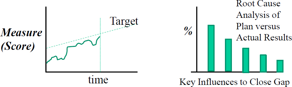
Source: Katzorki Nussle 1999.
- Take action based on the root cause analysis results using a new understanding of what factors drive plan results to be different from what was planned. This can include adapting or updating the plan and strategies accordingly.
Usage of Planning Frameworks and Methods in Transportation
Transportation agencies have utilized the above types of approaches and capabilities in similar ways as industry. Table 2 summarizes a selection of recent cases that demonstrate usage and successes of these frameworks and methods.
Table 2. Examples of Practice – Frameworks and Methods in Transportation
| Example from Practice | Description | Techniques Used |
|---|---|---|
| New York State: Long-term impacts of shared, connected, automated, and e-mobility (NYSDOT, 2020) | Planning and analysis study of autonomous vehicle evolution and future planning in NY State. | The study employed assessment of metrics, causal analysis of influences, modeling of plausible futures and scenario analysis, and assessment of challenges and opportunities. |
| Wyoming: Managing risks in project delivery (FHWA, 2013). | Effort to manage problems affecting Wyoming DOT’s ability to deliver projects on time and as intended. Investigated causes and avenues for improvement both in terms of planned actions and in terms of reducing uncertainties. Example of an effective qualitative approach. | This study used causal analysis to study the effects of various influences on outcomes, including uncertainties. (See Table 3 and Figure 14). This led the investigators to analyze project cost estimates from early reconnaissance to the letting date. As a result, they discovered influences like “gold-plating” projects that were firmly in the pipeline and “low-balling” new project costs that were reinforcing the influences and |
| decisions that caused important projects to be shelved. | ||
| Arizona Management System (Pounds, 2022) | Series of activities undertaken by ADOT starting in 2015 with the launch of the Office of Continuous Improvement (OIC) to work towards constant learning and improvement and to address hindrances in existing processes and tools. | ADOT uses the “Plan, Do, Check Act” (PDCA) cycle, and refers to it as their “mantra:”. They use the cycle for problem solving as well as root cause analysis, metrics tracking, and overall process analysis and improvement. |
| Michigan Mobility 2045 (Michigan DOT, 2021) | Statewide long-range transportation plan that included a scenario planning process to explore four alternative futures organized around the two axes of technology adoption (hi/low) and growth (hi/low). | This study used a mix of qualitative and quantitative scenario planning processes, including workshops to identify key sources of uncertainty and modeling in the statewide travel demand model of different patterns and levels of future growth and CAV technology adoption. The exercise identified how future CAV adoption could potentially have as large an increase on VMT growth as plausible high economic growth scenarios, pointing to the need to monitor this trend. The scenarios reinforced the general resilience of the network to increases in demand, confirming an emphasis on preserving and maintaining the existing network. A strategies workshop around scenarios also pointed to greater focus on partnerships and on hiring staff with data science skills. |
Table 3. Qualitative and Linear Causal Analysis of Influences on Project Deliveries from WYDOT
| Causes | Effects | Results | Candidate Strategies |
|---|---|---|---|
| Root Causes of Delays -- Low project cost estimates Inaccurate revenue projections Inaccurate inflation projections Uncertain funding | Revenue shortfalls. Over-programming of projects | Project splits Cost Escalation Downscoping Project Delays Increased crashes Redesign costs Lower performance | Pipeline loading Design time reduction “Critical Project” method TAM process improvements Revenue “smoothing” Org. response fixes PCS enhancements |
| “Hurry Up” Projects -- Volatile funding, Stimulus funds, “One-Time” infusions from the State, etc. | 1R2Rs get attention and get delivered. 3R4Rs pile up on the shelf and risk being delayed | ||
| Organizational Responses -- Beefing up projects already in the pipeline Tendency to provide low estimates “Early PCS” approach | Continued over-programming and project delays |
Source: FHWA (2013).
In addition to specific examples from practice, there is a range of research, guidebooks, and toolkits that apply similar frameworks and methods for specific purposes. The U.S. Climate Resilience Toolkit, for example, contains many resources aimed at developing resilience plans, including focused content around assessing vulnerability and risk (NOAA, n.d.). NCHRP Project 20-125 Strategies to Incorporate Resilience into Transportation Networks includes scenario planning as one method to support the building of network resilience (TRB, n.d.). Currently in-progress NCHRP Project 23-26 Impacts and Performance of State DOT Resilience Efforts is a research effort to help DOTs “check” the effects of resilience activities by identifying resilience performance measures across different asset classes and developing an approach that uses these measures to assess the effectiveness of resilience strategies. NCHRP Report 706, Risk Management and Data Management to Support Target-Setting for Performance-Based Resource Allocation by Transportation Agencies, discusses the analysis of performance metrics, including the impacts of uncertainty (Cambridge Systematics, Inc., 2011). Similarly, NCHRP Report 658, Guidebook on Risk Analysis Tools and Management Practices to Control Transportation Project Costs, offers support for quantifying the effects and impacts of uncertain threats (Molenaar et al., 2010).
Managing Deep Uncertainty: Joining Qualitative and Quantitative Approaches
Tough questions often accompany longer time horizons in planning. Typically, the future is more difficult to imagine than making simple projections or extrapolations from what is currently occurring or what has happened historically. “Uncertainty” frequently involves more than just one or two parameters that can be readily understood in formulating potential future scenarios. Moreover, it may not be possible to define or agree upon anything approaching a probabilistic distribution of potential outcomes. There can often be unintended consequences when implementing plans, including unanticipated effects of positive or negative feedback loops. These types of situations—which are very common in transportation planning—are sometimes referred to as “deep uncertainty” (DMDU Society, 2023).
An example of this would be the impacts of adoption of autonomous vehicles. According to one researcher at the National Renewable Energy Laboratory (NREL), who has been studying autonomous and/or shared vehicle futures for years, “We still do not know whether VMT will go up or down as a result of the advent of autonomous vehicles” (Sperling, 2019). Hence, the unknowns in the adoption of these vehicles are still significant.
So, what additional capabilities may be helpful in leveraging the basics of PDCA and basic causal diagrams for dealing with “deep uncertainty”? These types of capabilities would require more sophisticated methods and/or rigor, due to the inability to anticipate a range of coherent, plausible “futures”, especially for longer range plans. Dealing with high situational complexity requires the consideration of a full range of influences on outcomes, including identifying and analyzing potential feedback from proposed actions, and managing the possibility of there being a range of eventual scenarios. Depending upon the complexity of the situation, there may be
value in combining insights from a thorough qualitative causal analysis with more quantitative approaches such as simulation.
Illustrative Example: Managing Deep Uncertainty Using Scenario Analysis and Simulation
The following section walks through an illustrative example of how qualitative and quantitative methods can be used in combination to support understanding of and planning for uncertainty.
Basic causal analysis can be well utilized to depict a range of possible “futures” related to your plan. Once laid out, this analysis can be a useful framework and diagnostic for discovering how plans may unfold. Moreover, the use of causal analysis allows you to define and analyze a range of outcomes that could apply to the situation, including the impacts of risks and uncertainties that might exist.
For example, Figure 13 is a causal diagram of CAV adoption in a metro area (Redd, 2018). The purposes of the diagram were to capture key influences on CAV adoption and how they interact, in order to understand possible future scenarios, and to potentially support actual simulation of the overall environment. Specifically, the approach was useful in identifying a range of scenarios across a spectrum of highly variable and uncertain influences.

Source: Redd 2018.
Figure 14 shows how a range of “plausible futures” for CAV adoption may exist as a result of implementing a given plan. Specifically, if your causal analysis could possibly lead you in more
than one direction in terms of outcomes, it is important to identify those potential scenarios. The “secret” or “art” in doing so involves making sure each scenario is “coherent.” In other words, in the identification and depiction of a possible scenario, it is important to “tell the story”, and assure that the influences being considered in the analysis are holistically compatible in terms of how they drive outcomes in ways that make sense. This technique will allow the analyst to cut through large amounts of complexity, and create plausible futures that each involve realistic, but still uncertain and varied futures. Once established, these coherent scenarios can be used to manage the plan, and perhaps be quantified to some extent to provide more confident insight.

Source: Redd 2018.
Lastly, it may be helpful in some situations to quantify how things may “play out” over time through the use of modeling or simulation. The act of attempting to add numbers to the driving influences and quantify results can add realism and at least some further understanding of a situation, regardless of the fear of “being wrong.” But the ability to perform sensitivity studies of the effects of driving influences over realistic ranges can provide tremendous insight and perhaps direction in planning.
Figure 15 shows an example of CAV adoption simulation results from the causal analysis described above. The figure shows an actual quantification of the CAV adoption environment, based on a set of reasoned assumptions for the model. This provides an example of how various parameters behave (together) over time, and how they affect bottom-line results that planners are trying to understand.
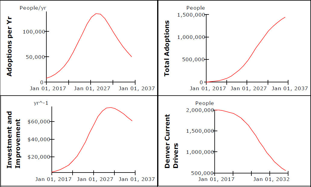
Source: Redd 2018.
Emerging and More Advanced Approaches
Within the spectrum of more quantitative approaches, there are a number of methods being developed and tested that are as of yet not embedded in practice but may provide new opportunities.
Decision-Making Under Deep Uncertainty (DMDU) refers to a collection of methods and tools that planners can use to migrate away from a “predict-then-act” framework to one that is focused on stress testing strategies to different futures and thereby learning to revise plans or identify new strategies (Figure 16). For example, the Sacramento Area Council of Governments (SACOG), through simulations over many plausible futures, used DMDU to examine which external trends are most likely to threaten its ability to meet future greenhouse gas emissions reductions goals (FHWA, 2022c; Lempert 2022).
Other advanced and emerging approaches include Robust Decision Making (RDM), Info-Gap Theory, and Dynamic Adaptive Pathways Planning. Robust Decision Making, unlike Monte-Carlo Simulation which takes a probabilistic approach to expected outcomes, helps policymakers identify robust strategies by using simulations to stress-test them under many conditions (Zmud et al., 2018). RDM is adaptive and can evolve over time as it receives new information. Once strategies are evaluated, analysts can identify which types of scenarios a given strategy performs poorly in, and make strategy adjustments to enhance resilience to that class of scenario (Lempert
et al., 2022). Info-Gap Theory, in contrast to RDM, uses models to see how options perform as a function of uncertainty (Zmud et al., 2018). The output of Info-Gap Theory is usually in the form of a graph that allows the decision makers to see what level of performance can be achieved as a function of uncertainty on the other axis highlighting trade-offs, risks, and vulnerabilities of each outcome (Zmud et al., 2018). Lastly, Dynamic Adaptive Pathways Planning conceptualizes series of different actions over time which provides different pathways, as the name suggests. By exploring path-dependency of actions, decision makers can design adaptive plans for short-term as well as long-term actions and also consider plan reassessment as needed.

Source: FHWA (2022).
3. Data and Methods to Assess Uncertainty and Its Impacts
Introduction
This chapter addresses data, methods, and tools that are widely available to transportation agencies to address the effects of uncertainty. Uncertainty is present in many of transportation agencies’ functions broadly defined by time horizon (from immediate decisions to multi-decade plans), transportation modes, and goals. The unifying thread is that the data, methods, and tools in this subsection can each help transportation agencies address their common functions related to the types of uncertainty addressed in the prior subsections.
Some of these transportation agency functions have more data, methods, or tools for addressing the effects of uncertainty than others, and some are more accessible to agencies with more funding or technical capabilities. This subsection reflects these differences by focusing on some of the most developed or accessible data, methods, and tools, delving most deeply into the
functions that have the most resources and highlighting gaps where few or no practical resources exist. Furthermore, this section does not seek to exhaustively inventory all resources for transportation agencies to address the effects of uncertainty. It instead focuses on those that are the most developed or are most likely to be helpful rather than on theoretical research or emerging methods.
The data, methods, and tools described help agencies account for uncertainty in different parts of their work. For example, they can help make agencies’ asset management plans more resilient to environmental changes, they can help identify airports at risk of major decreases in commercial aviation activity, and they can identify risks to agency business processes and provide a framework for developing mitigation strategies. These approaches can sometimes help distinguish high-probability / low-impact events from lower-probability / higher-impact events. Even where uncertainty cannot be captured probabilistically, these approaches can be used to explore the boundaries of potential outcomes and impacts.
Following this introduction is a summary section that describes the types of resources available to transportation agencies. Then, the report addresses resources for assessing uncertainty and its impacts organized within two broad categories of transportation agency functions:
- Infrastructure: Design, construction, maintenance, preservation, and management of physical transportation assets, such as roads and bridges.
- System performance: Multimodal transportation operations, including topics such as highway operations, safety, freight movement, non-highway transportation operations, and environmental impacts on transportation system operations.
Summary of Data, Methods, and Tools
This subsection describes tools, data sets, or methods. Table 4 below lists methods and Table 5 lists tools and data sets, which are presented together because many tools produce data sets. This document generally focuses on categories of tools and data sets, only citing specific tools and data sets that are very common or well known to illustrate the category. The greatest number of data, methods, and tools relate to infrastructure and system preservation, with a focus on highway infrastructure and automobile transportation over other types of infrastructure and modes.
Table 4: Summary of Methods
| Name | Description | Common Applications |
|---|---|---|
| Risk Management | Risk management involves identifying and assessing risks, as well as developing procedures to reduce their likelihood or mitigate their impacts | Asset management, highway and non-highway system performance |
| Sensitivity Analysis | Sensitivity analysis involves examination of the range of impacts that a variation in a given variable can have on an outcome. | Many quantitative/mathematical models, such as asset management models and travel demand models |
| Name | Description | Common Applications |
|---|---|---|
| Life-Cycle Analysis | Life-cycle analysis involves examination of the activities to preserve an asset and costs associated with these activities. | Asset management |
| Scenario Planning | Scenario planning involves the analysis of and preparation for multiple potential futures. | Asset management, highway and non-highway system performance |
| Use of contingency factors | Contingency factors can be added to a budget to account for unknown costs. | Estimation of project costs |
| Monte Carlo methods | Monte Carlo methods rely on repeated random sampling. | Estimation of project costs, comparison of scenario risk (e.g., climate impacts, hurricane exposure) (Zhu et al., 2018), high-level travel demand modeling (Hong and Najmi, 2022) |
| Visioning and Sketch Planning | Visioning tools help stakeholders develop a share vision for the future, while sketch planning tools aim to produce estimates of direction and order of magnitude of an outcome. | System operations and performance, although this method has wide-ranging applications |
| Decision Science and Tradeoff Analysis | Decision science involves a set of techniques to inform decision making. Tradeoff analysis examines the relative utility of different outcomes to decision makers in a given situation. | System operations and performance, although these methods have wide-ranging applications |
| Exploratory Analysis | Exploratory analysis is intended to uncover interactions or potential relationships among variables for further study. It is often contrasted with predictive analysis that builds off of known relationships among variables to forecast a future (Holdaway, 2014). | System operations and performance, although this method has wide-ranging applications |
Table 5: Summary of Data Sets and Tools
| Name | Description | Common Applications |
|---|---|---|
| Pavement Management Systems | Pavement management systems assist in pavement management decisions, often by storing data on pavement inventory and conditions, storing information on inspections, forecasting pavement condition, and selecting optimal preservation activities. | Pavement asset management |
| Bridge Management Systems | Bridge management system assist in bridge management decisions, often by storing data on bridge condition and inspections, forecasting bridge condition, and selecting optimal activities to maintain a state of good repair. | Bridge asset management |
| Transit asset management systems | Transit asset management systems store condition data and maintenance activity, prioritize maintenance and replacement activities within limited funding, and calculate investment needs. | Transit asset management |
| Visioning and sketch planning tools | Visioning tools help stakeholders develop a shared vision for the future, while sketch planning tools can illustrate the types, direction, and size of impacts of external factors and agency strategies on outcomes. VisionEval is a commonly used open-source visioning and sketch planning tool. | Multimodal mobility |
| Name | Description | Common Applications |
|---|---|---|
| Travel demand models | Travel demand models predict future travel activity within their modeling region under specified conditions. While many travel demand models are highway-focused or multimodal, there are also travel demand models focused on transit, such as the Simplified Trips-on-Project Software (STOPS). | Highway and multimodal mobility Transit system operations and performance |
| Freight models | Freight models predict freight movement within their modeling region under specified conditions. | Freight mobility |
| Decision science, tradeoff analysis, and exploratory modeling tools | Rhodium is an open-source Python library that provides tools for decision science, tradeoff analysis, and exploratory modeling. Transportation Model Improvement Program (TMIP) Exploratory Modeling and Analysis Tool (EMAT) is an exploratory modeling and analysis approach that is particularly focused on uncertainty in transportation systems that arises from technological advancements. | System operations and performance, although this method has wide-ranging applications |
| Freight forecasts | Freight forecasts show projections of future freight movement based on origin-destination fairs or assigned to transportation networks. The Freight Analysis Framework (FAF) is one of the most used freight forecasts. This free data set models and forecasts freight movement across several freight modes. There are several data tools that can be used to access the underlying data. | Freight system operations and performance |
| Airport weather-related tools | These tools can help airport managers understand how climate or weather events may affect airport infrastructure and operations. The Airport Weather Advanced REadiness (AWARE) toolkit can help show the effects of rare weather events on airports. The Airport Climate Risk Operational Screening (ACROS) tool helps airports identify airport components that are at risk from the climate. | Airport management |
| Environmental impact forecasting tools | Several tools exist to forecast exposure to or impacts of environmental hazards in different weather scenarios (e.g., hurricane impacts) or climate scenarios. For instance, the Vulnerability Assessment Scoring Tool (VAST)is a tool that guides users through a quantitative, indicator-based screening of vulnerabilities of the transportation system. The CREAT Climate Change Scenarios Projection Map shows climate-related risks to water provision and utility operations. Hazus estimates risks from earthquakes, floods, tsunamis, and hurricanes. | Environmental impacts |
Specific Data, Methods, and Tools
This section details the most developed or prevalent data, methods, and tools that transportation agencies can use to address uncertainty in transportation. The data, methods, and tools are grouped into categories around transportation infrastructure, system operations and performance, and transportation agency policies.
Infrastructure
Maintaining infrastructure to ensure safe operations is at heart of what transportation agencies do. Their experience has translated into fairly developed set of tools and techniques to quantify the performance implications of uncertainty. This section summarizes the data, methods, and data for accounting for uncertainty in infrastructure decision making that already exist in practice.
Uncertainties cover the spectrum of design, construction, operations, preservation, and maintenance activities. This section is organized according to national guidance on mitigating adverse impacts from uncertainties, followed by analytical techniques used to determine the range of likely outcomes, and how the techniques have been implemented throughout typical asset management business functions. This range of potential outcomes is then used to inform the risk monitoring process and considered when deciding on policy decisions.
Transportation agencies can address uncertainty at several levels within their business processes. These range from organizational-level strategies to the selection and implementation of projects and activities. The following subsections describe the data, methods, and tools available to transportation agencies to manage uncertainty in infrastructure management at each of these levels.
Organizational Strategies to Account for Infrastructure-related Uncertainties
Organizational strategies refer to the ways in which organization leaders decide to structure the organization and implement high-level policies and processes to guide the use of the organization’s resources and energies to address uncertainty. The Moving Ahead for Progress in the 21st Century Act (MAP-21) requires risk-based Transportation Asset Management Plans (TAMPs) and Transit Asset Management (TAM) plans with requirements for both highway infrastructure (i.e., pavement and bridges) and transit assets respectively. State DOTs and transit agencies are required to identify risk strategies as a condition of receiving federal funding. Since risk assessment is one of the major approaches that organizations deploy to manage uncertainty, the following paragraphs detail data, methods, and tools to develop systemic risk-based asset management plans.
Risk Assessment and Management for Transportation Asset Management Plans (TAMPs)
The International Organization for Standardization (ISO) has defined a series of steps in the risk management process. Table 6 below describes the different methods and tools that states use for each of these steps, as characterized by Liu and McNeil (2020). TAMPs typically include processes for risk as it relates to an organization’s physical infrastructure and its maintenance. These processes include identifying and assessing, analyzing, mitigating, and monitoring. Common categories of risk include environmental, cybersecurity, operational, and financial risk.
Table 6: Methods and Tools for Risk Management
| Steps | Tool and Description |
|---|---|
| Context Setting | Exercise: Form teams, assign risks, clarify objectives and environment |
| Risk Identification | Workshop*: Workshops are designed to engage experts in identifying risks using techniques such as brainstorming, interviews, Delphi, checklists, scenario analysis, cause and effect, and categorization |
| Risk Analysis | Understanding cause and effect: Usually based on expert judgment Likelihood of the risk*: May be qualitative or quantitative; set levels; build likelihood table Consequences: May be qualitative or quantitative; set levels; build consequence table Risk*: Risk is the product of likelihood and consequences; assemble risk matrix Determine cause: Managing the cause, conducting analysis workshops and work groups, bow-tie analysis (implemented in the framework of a diagram describing the causes [left side of the bow] and consequences [right side of the bow] of an event), structured what-if technique, root cause analysis, Monte Carlo simulation Risk score: Established a numerical score reflecting the probability of the event combined with the severity of the impact Risk map: Color code risk matrix |
| Risk Evaluation | Risk appetite: Sets threshold or tolerance for risk. May be value-based, program-based, cost-based, risk score-based, or asset-based Risk prioritization*: May be policy-based, cost-based, or based on secondary benefits or impacts |
| Risk Management | Five T’s: Tolerate, treat, transfer, terminate, take advantage of Three R’s: For catastrophic and disaster events: robustness (capacity to cope with stress), redundancy (alternative strategies), and resiliency (absorb, recover, adapt) |
| Communication, Monitoring, and Feedback | Risk registers*: Summarize the outcomes from the preceding steps Scorecards: Keeps track of activities Risk indicators as metrics: Integrates risk management with key agency business activities (e.g., target setting, performance management) |
Source: Adapted from Liu and McNeil (2020) * Indicates the most commonly used tools by state DOTs in TAMPs as described by Liu and McNeil (2020)
Risk assessment can also be used to identify the risk of bridge failure. Three common techniques for analyzing risks of failure include expert opinion (used when there is limited data), reliability analysis (used when there is not data on past failures), and failure analysis (based on analysis of historical data). Reliability analysis uses simulations of the bridge’s performance with different loads and conditions to estimate failure risk, while failure analysis applies statistical analysis to historical data on prior failures (Cook, 2014; Bulleit, 2008; Paté-Cornell, 1996).
Analytical Approaches for Quantifying Uncertain Outcomes
Many studies have detailed methods to quantify the performance implications of uncertainty on transportation infrastructure through a variety of models. In general, the choice of analytical approach depends on the type of uncertainty that the agency is assessing. Epistemic uncertainty (often simply called “uncertainty”) exists due to a lack of knowledge about a system’s workings, while aleatoric uncertainty (often called “risk”) relates to inherent variability and randomness associated with a system (Guo & Du). As described below, sensitivity analysis is generally used to
describe variations in outcomes due to epistemic uncertainty, while life-cycle analysis and other probabilistic approaches are used to account for aleatoric uncertainty.
Sensitivity Analysis
Sensitivity analysis assesses “uncertainty that quantifies how outputs may change when input values are systematically varied on a unit-by-unit basis” (Ford et al., 2012b). Sensitivity analysis techniques are the most commonly applied for quantifying the repercussions of epistemic uncertainty. Most commonly this calls for ‘swinging’ explanatory factors across a range of possible values with an assumption of holding constant all other factors.
Using sensitivity analysis when forecasting infrastructure conditions or developing asset management plans can help identify risks where changes in modeling assumptions (e.g., faster than expected deterioration of assets related to usage, precipitation, or temperature; lower than expected funding) can have major implications for resulting asset conditions (Ford et al., 2012). Sensitivity analysis is especially useful when inputs into a model are difficult to precisely estimate, increasing the uncertainty in model outputs. Sensitivity analysis allows model inputs to be varied to show the range of outputs that may be obtained and the variables that have the greatest impact on model outputs (Tobin and Friesz, 1988). One of the useful outputs of sensitivity analysis are “tornado diagrams,” which graphically depict a variables’ influence on outcomes as “the correlation between variations in model inputs and the distribution of the outcomes” (Molenaar, 2010). As illustrated in Figure 17, tornado diagrams derive their name from the fact that the longer bars at the top of the diagram, indicating in this case that the activity poses a greater likelihood of prolonging the schedule (or more generally pose greater risks), give the diagram the form of a tornado silhouette.
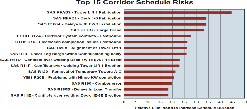
Source: Molenaar, 2010.
Asset Management Decision Making
Asset management decision making frameworks typically include life-cycle analysis, deterioration modeling, and financially-constrained work plan development. Pavement and bridge management software and transit asset management systems facilitate these steps for agencies for pavement, bridges, and transit assets respectively.
Pavement and bridge management software stores information about asset inventory and condition, track inspections and store inspection information, can forecast future conditions given a certain set of preservation activities, and can develop optimal sets of preservation activities within constraints provided by the agency. Transportation agencies operate pavement and bridge management software that they have developed themselves and that they have purchased from vendors.
Transit agencies build, operate, and maintain numerous assets, which depending on the type of transit may include vehicles, fixed-rail infrastructure, maintenance facilities, and bus and train stations among other asset types. Transit asset management systems help transit agencies track current asset condition, forecast asset condition, and select optimal treatments. One of the most common transit asset management systems is the Transit Economics Requirement Model (TERM) by the Federal Transit Administration (FTA). TERM provides a national-level analysis of asset conditions, state of good repair backlog, and 20-year reinvestment needs. TERM-Lite allows agencies to simulate asset conditions under different constrained funding amounts. Thus, agencies may account for uncertainty in funding availability by developing different funding and investment scenarios for which TERM-Lite can estimate assets future condition and backlogs in a state of good repair (FTA, 2019; FTA, 2013a).
Life-Cycle Analysis
Probabilistic risk analytical techniques are most often used to quantify the impacts of aleatoric uncertainty. Probabilistic risk analysis calls for simulating the joint probability distribution of independently modeled uncertainties. Probabilistic assessments are based on an examination of factors affecting the outcome of interest to an agency, such as asset life, and the way in which uncertainty propagates into subsequent processes (Ford et al., 2012). They can be used to quantify the level of confidence that an activity will be cost-effective based on probabilistic estimates of life. Pavement and bridge management software (including AASHTOWare’s Bridge Management (BrM), which is a widely used bridge management software (BMS)) can support lifecycle analysis of risk under conditions of changing traffic loads, environmentally related deteriorate rates (e.g., due to precipitation, temperature), and budget allocations. Different scenarios can be assembled for each of these, and assets experiencing the greatest deterioration can be identified, showing those assets’ risk levels (Fiorillo and Ghosn, 2022).
Deterioration Modeling
Usage of highway and transit infrastructure, particularly usage in non-ideal precipitation, temperature, other environmental, or usage conditions may create risks for the infrastructure and
shorten their life. Using asset management tools that forecast pavement or bridge deterioration based on historically derived deterioration rates and optimized treatments and activities allows asset managers to show network-level risks for different expenditure levels and ways of assigning activities (e.g., ‘worst first,’ lowest life cycle cost) (Fiorillo and Ghosn, 2022). Deterioration modeling may also leverage previously described methods such as sensitivity analysis and risk assessment (Ford et al., 2012) to show, for instance, the effect that elements such as usage, soil corrosiveness, precipitation, temperature, and location can have on bridge and culvert service life (sensitivity assessment) or to develop confidence intervals for service life (risk assessment) (Ford et al., 2012).
Environmental and Extreme Event Risk
Environmental and extreme event risk assessments can show hazards that may disrupt infrastructure, including bridge and pavement infrastructure. Risk assessment can often be integrated with asset management systems’ assessment of benefits and costs (AASHTO Standing Committee on Highways, 2016a). The final report for NCHRP 20-07 (378) has documented how transportation agencies account for risk in their asset management decision making and also provides a series of risk assessment work sheets that calculate a vulnerability index and a social cost of risk for bridges associated with potential hazards to bridge infrastructure such as landslides, floods, scour, wildfires, and usage by overweight or overheight vehicles (AASHTO Standing Committee on Highways, 2016a). The spreadsheets and framework provided by NCHRP 20-07 (378) use estimates of the likelihood of extreme events (e.g., earthquakes, floods), the likelihood of transportation service disruptions of these and other events including scour and overheight collisions, and the consequences of that service disruption to calculate vulnerability, resilience, and social cost of risk (AASHTO Standing Committee on Highways, 2016b). Additionally, some asset management tools provide a framework for applying risk models, including AASHTOWare Bridge Management (BrM). In BrM, risk is assessed at the level of individual bridges, whereby bridge inspectors may note risk-related concerns associated with bridges which are recorded with that bridge’s record in BrM. This is a concrete example of risk assessment being built into asset management systems since the system allows inspectors to enter risk-related concerns into the system using a numerical rating system for both the likelihood of a hazard and the severity of its consequences (AASHTO Standing Committee on Highways, 2016b).
Construction Costs
While there are numerous data sets, methods, and tools for managing and preserving transportation assets, transportation agencies encounter uncertainty well before the asset management stage of assets’ life-cycle. Indeed, there is significant uncertainty in assets’ design, bidding, and construction phases. Transportation agencies need to estimate project costs. This is done first in the planning phase and proceeds through programming, preliminary design, final design, advertising and bidding, and construction. At each phase, the construction cost estimates become more precise because more information is available about the project (Molenaar et al., 2010). The accuracy and comprehensiveness with which transportation agencies scope projects
at early phases will affect their ability to deliver the project on time and on budget. For most agencies, project scoping begins in the planning phase and ends in either the preliminary or detailed design phases (Molenaar et al., 2010). Although transportation agencies define and approach project scoping very differently, it is often possible for them to improve the accuracy of their scoping process by involving experts from multiple functional disciplines, using multiple tools and data sets to support the scoping process, and allocating adequate time and resources to complete project scoping (Molenaar et al., 2010).
Agencies may use risk management for estimating and managing project construction costs. As described by the Molenaar et al. (2010), risk management involves risk identification, risk assessment/analysis, risk mitigation and planning, risk allocation, and monitoring and control. These steps are roughly analogous to those described by Liu and McNeil (2020) around asset management in Table 6 above. These risk management steps can be applied to each stage of the cost estimation and refinement processes in planning, programming, and design, as summarized in Table 7 below. Similar risk management frameworks have been promoted by federal agencies (FHWA, 2018) and have been implemented for managing project risks by transportation agencies (Oregon Department of Transportation, 2019; Washington State Department of Transportation, 2018).
Table 7: Risk Management Framework Relationship to Project Phases
| Risk Management Step | Planning | Programming | Design |
|---|---|---|---|
| Risk identification | Identification of highest-level risks to project scope and feasibility | Complete and nonoverlapping identification of risks for baseline project estimate | Appraisal of identified risks Identification of new risks as design progresses |
| Risk assessment / analysis | Initial ranking of risks Order of magnitude risk costs and total cost range | Qualitative analysis / ranking of risks on minor projects Detailed quantitative risk analysis on major projects Contingency for baseline cost estimate | Updating of qualitative or quantitative risk analyses Updating/resolution of contingency |
| Risk mitigation and planning | Initial development of red flag list, risk register or formal risk management plan | Finalization of risk register or risk management plan Tradeoff analysis for mitigation options | Completion of risk management plan Continued tradeoff analysis for risk mitigation options |
| Risk allocation | Initial analysis or selection of project delivery method | Trade-off analysis for risk allocation (e.g., contract provisions for time, payment, delay, etc.) | Final risk allocation in contract provisions |
| Risk monitoring and control | Planning for risk monitoring and control | Implementation of risk register or risk management plan | Active management of risk register or risk management plan |
| Risk Management Step | Planning | Programming | Design |
|---|---|---|---|
Establishment of key risk management milestones | Active management and resolution of contingency |
Source: Molenaar et al., 2010.
In estimating project costs, risk analysis has both traditional methods and more complex methods that can help. Traditional methods for estimating cost determine point-estimates values for construction contingency (Hoseini et al., 2020). Traditional methods develop a cost contingency based on the probability of certainty costs and their likely cost, where the contingency is the sum product of costs and their probabilities (Molenaar et al., 2010). Whether developed this way or another way, the cost contingency is intended to be added to the base cost of the ‘known knowns’ related to the project and to account for the ‘known unknowns’ and the ‘unknown unknowns’ (Hoseini et al., 2020). It is also possible to consult experts to develop the most likely values, and upper and lower ranges for cost estimates (Galway, 2007). These methods contrast with other probabilistic methods that can explicitly incorporate uncertainty into the contingency cost estimates (Hoseini et al., 2020). More complex methods such as Monte Carlo simulation require users to provide information about the probability distribution of cost components and can produce project-level probability distributions showing the costs that are most likely as well as high and low estimates (Molenaar et al., 2010). These distributions can be narrowed as costs become more certain. An example of a project-level probability distribution from a Monte Carlo simulation is shown in Figure 18.

Source:Molenaar et al., 2010.
Other Topics
There are of course other infrastructure-related topics where transportation agencies face uncertainty. These include but are not limited to bid amounts, construction time, labor disruptions, changes in the price of materials and work, and contractor availability. While these and other areas of infrastructure-related uncertainty impact transportation agencies; methods, data, and tools for addressing uncertainty related to them are less developed in the state of the practice than for the areas highlighted above.
System Operations and Performance
System operations and performance relates to the operations of transportation systems across modes (e.g., highways, transit, rail) and purposes (e.g., passenger movement, freight movement, recreation). It encompasses such topics as highway mobility, safety, freight movement, non-highway system performance, and environmental disruptions. Transportation agencies encounter both epistemic uncertainty and aleatoric uncertainty in managing system performance. This section summarizes key data sets, methods, and tools for addressing uncertainty in system performance, organized around uncertainty in highway mobility, non-highway system performance, and the environment. Although environmental events (e.g., storms, earthquakes, forest fires, dust storms) may affect both highway and non-highway mobility, environmental events are addressed in separate section because of the existence of numerous data sets, methods, and tools focused on environmental uncertainties.
There are several types of data, tools, and methods that can help transportation agencies account for uncertainty in system operations and performance. Many of these categories of data, tools, and methods can address uncertainty across multiple modes or do not require mode-specific inputs.
Visioning and Sketch Planning Tools
Visioning tools help stakeholders develop a shared understanding vision for the future. Sketch level planning tools can provide stakeholders with a broad understanding of the types, direction, and size of impacts of external factors and agency strategies on future outcomes. They are often used in concert with scenario planning approaches.
VisionEval is one such visioning and sketch planning tool. VisionEval provides a fast, high-level strategic model for regional and statewide transportation organizations (Collaborative Development of New Strategic Planning Models Pooled Fund, 2023). Whereas tactical and operational models utilize fixed assumptions to model and make decisions on funding and implementation, strategic models such as VisionEval sacrifice detail to better explore potential futures for long-range visioning, policy-making, or resilience analysis. VisionEval takes inputs such as future population characteristics or transportation mode splits and employs elasticities between various factors to facilitate evaluation of many potential futures created by combinations of factor assumptions. Other sketch planning methods utilize even simpler
frameworks such as excel-based worksheets to explore and combine different factors affecting future system performance.
Travel Demand Model
Many transportation agencies have travel demand models used for forecasting capacity needs and highway mobility conditions. In a some but not all cases, these models are multimodal and inclusive of transit or non-motorized modes. These travel demand models are subject to uncertainty in their model inputs. For example, long-term demographic and economic forecasts are inherently uncertain. Travel survey-generated data used to support model calibration are also subject to uncertainty due to sampling bias, and bias produced by the survey design (Rasouli and Timmermans, 2012). Moreover, behavior and preferences can change over time, with data describing these things always lagging. It is possible to account for uncertainty through the use of scenarios that differ in the configuration of their inputs or by sensitivity analysis similar to the sensitivity analysis conducted for infrastructure assets (described on page 52).
Decision Science and Tradeoff Analysis
Tools for decision science inform decision making through a series of quantitative methods, which may include tradeoff analysis. Rhodium is an open-source Python library that provides tools for decision science, tradeoff analysis, and exploratory modeling (EM) (Project Platypus, 2023). Rhodium aims to identify robust strategies, characterize vulnerabilities, and evaluate tradeoffs. Rhodium can interface with models built in a variety of languages, including Python, R, and Excel. By defining aspects such as constraints, levers, uncertainty, and responses, users can better understand the performance of strategies across a wide range of scenarios. Although the known research does not cite any instances of the package being implemented for transportation planning in the U.S., several research articles on sustainability and climate resilience have cited the software and the associated paper in the Journal of Open Research Software (Hadjimichael et al., 2020).
Exploratory Analysis
Much like Rhodium, the Transportation Model Improvement Program (TMIP) Exploratory Modeling and Analysis Tool (EMAT) is designed to identify robust strategies and evaluate tradeoffs. It also provides exploratory analysis meant to uncover potential interactions for further study. FHWA’s TMIP started in 1994 and supports transportation professionals’ efforts to better represent their respective systems through products such as their travel analysis toolbox and the TMIP Exploratory Modeling and Analysis Tool (EMAT) (FHWA Travel Model Improvement Program, 2019). TMIP EMAT is an exploratory modeling and analysis approach that is particularly focused on uncertainty in transportation systems that arises from technological advancements. TMIP-EMAT’s purpose is to “help agencies manage uncertainties by illuminating interactions between transportation supply and demand on urban surface transportation system through exploratory modeling and simulation; provide insights of potential, possible, plausible, probable or preferred futures; and support robust regional transportation planning decision-making
incorporating principles of risk management” (FHWA, 2019). Because there is a wide range of unknowns related to this topic, EMAT runs other transportation models, adjusting their parameters to simulate hundreds or even thousands of possible scenarios. This produces a meta-model that can then be used to show the potential impact of various policy decisions on system performance outcomes. The development project conducted testing of the system with Oregon DOT using its activity-based model in VISUM, San Diego Association of Governments using its Emme-based sub-regional analysis model, and the Greater Buffalo Niagara Regional Transportation Council using its TransCAD trip-based model (FHWA, 2019).
Freight
Transportation agencies may need to forecast freight movement to prepare the transportation system for freight-related demand. Freight-related uncertainties include reconfigurations of the supply chain (e.g., nearshoring) that change origins or modes of freight movement, changes in demand for goods by consumers, and labor issues (e.g., strikes). These uncertainties may affect multiple modes including trucking, freight rail, ports and waterways, and air cargo. TRB research has developed a framework for transportation agencies to use to develop resilient supply chains that encompass the following steps (Meyer et al., 2019):
- Organize for success
- Develop a communications strategy/plan
- Assess current practice
- Understand the hazards and threats
- Develop strategies/actions
- Implement strategies and actions – note these may relate to system operations (e.g., enhance emergency response capabilities) and capital improvements.
- Monitor system performance
The same research also includes practical steps for transportation agencies to follow to implement the framework, which may include conducting pilot studies, collecting data on supply chain disruptions, conducting pre-incident resilience exercises, incorporating supply chains into emergency management exercises, establishing resiliency advisory committees for DOTs, developing resiliency performance measures, and others (Meyer et al., 2019). Many of these approaches are similar to risk management more broadly.
Some transportation agencies have freight models of various sorts that can be used for forecasting freight movement under different conditions. These models types may include truck models (which are truck-centric travel demand models), direct commodity table freight models (which produce truck trip tables from travel demand model outputs), economic freight models (which calculate demand and consumption of freight activity through an economic model), and four-step freight models (which produce truck trip tables through a traditional four-step model) (Travel Forecasting Resource, 2020). It is possible to use these models to account for uncertainty by developing scenarios with different configurations of these inputs or by conducting sensitivity
analysis. Depending on the model type, configurable inputs may include trip origins or destinations, future population and employment, fuel price (Goulias et al., 2013), and network capacity (Travel Forecasting Resource, 2020).
Additionally, one of the most commonly combined adopted resources for forecasting national freight activity, the Freight Analysis Framework (FAF), includes forecasts for three economic scenarios (low-growth, baseline, and high-growth), which can help users account for uncertainty in future economic performance (FHWA, 2022f).
Non-Highway System Operations and Performance
Transportation agencies also plan for, manage, and support non-highway system performance through modal plans, funding programs, and technical assistance among other means, including aviation, transit, rail, and active transportation. In doing so, they use a range of methods, data, and tools to help address uncertainty. While the tools for system operations and performance discussed in the prior section can be applicable to multiple transportation modes, this subsection discusses data, methods, and tools specific to the operations and performance of non-highway systems.
Aviation
One major way in which State DOTs conduct long-term planning in aviation is the development of statewide aviation system plans that forecast airport-level demand among other outputs. There is significant uncertainty in these forecasts which depend on elements such as passenger and cargo demand, airport investment and policies, and airline network configurations. Given this uncertainty, some statewide aviation system plans develop multiple scenarios to forecast aviation activity (Georgia Department of Transportation, 2018). Additionally, while less prevalent in the state of the practice, researchers have developed multiple methods for reducing uncertainty in airport planning by developing improved methods for identifying peer airports with similar socioeconomic trends, using a logistic regression model to predict airline hubbing changes that could affect airport activity, and improving airport activity forecasting accuracy by accounting for past forecasting errors (Suh, 2018). Adoption of these or similar technical improvements to existing forecasting techniques can help account for uncertainty by improving forecast accuracy.
There are also many tools, methods, and data sources to address the uncertain effects of environmental, weather, and climatic trends and occurrences on aviation. These may be used by aviation departments at State DOTs or by staff at individual airports. They include:
- The Airport Weather Advanced REadiness (AWARE) toolkit: The AWARE toolkit can help show the effects of rare weather events on airports and help assess airports’ readiness. It can help agencies address uncertainty by showing the weather events that airports may be exposed to and the potential costs associated with those weather events (ICF International et al., 2016).
- The Airport Climate Risk Operational Screening (ACROS) tool: ACROS helps airports identify airport components that are at risk from the climate and supports processes that are intended to help identify climate-related risks and potential adaptation measures (Dewberry et al., 2015). The Airport Cooperative Research Program (ACRP) subsequently developed practical guidance for identifying climate-related risks for airports, which can assist airports in using the ACROS tool (ICF et al., 2018).
Beyond seeking to identify risks and adaptation strategies, airports also have options for dealing with uncertainty by building facilities in ways that more easily allow them to flexibly change operations in the future (Chambers, 2007).
Transit
While some agency’s travel demand models are multimodal, particularly in regions with long histories of transit usage, it is also common in transit planning to rely on specialized transit modeling and forecasting tools. One of the commonly used models for predicting usage of transit routes is the Federal Transit Administration’s (FTA) Simplified Trips-on-Project Software (STOPS). The STOPS methodology is similar to that of other travel demand models, but with several steps adjusted to make it useful for transit and with varying options for local calibration without the need for full-blown local model development. STOPS can forecast transit usage and change in vehicle miles traveled (VMT) due to a transit project in ‘build’ scenarios with the project and ‘no-build’ scenarios without it. There is uncertainty in transit inputs similar to those for other travel demand models (documented on page 58). Since the tool does not account for uncertainty explicitly, it is best to account for it in how the tool is used, such as by developing scenarios with different inputs or conducting sensitivity analysis (FTA, 2013b).
Intercity Passenger Rail
As with other modes, intercity passenger rail planning relies on forecasts of demand to support planning of future investments in infrastructure and service. Demand and ridership depend on the conditions of service offered as well as the future configurations of many other elements that affect demand for rail service, including population growth, economic activity, cost and service of competing modes, and the details of the rail option’s service offerings. The most ambitious passenger rail project in the United States in the last decade has arguably been the California High-Speed Rail program. As such, it is an example of the tools and methods that have been used to manage uncertainty in passenger rail planning. The California High-Speed Rail Authority developed a model to forecast its ridership for different service options with separate long-distance and short-distance components (California High-Speed Rail Authority, 2016). The Authority recognized the great amount of uncertainty in its forecasts and employed a combination of risk-based modeling processes to address this. Specifically, it developed a range of ridership estimates by running the model 150 times with different inputs and then developing statistical relationships (a ‘metamodel’) between inputs and ridership that it could use to
extrapolate those 150 model runs into many times more configurations of inputs (California High-Speed Rail Authority, 2020).
The California High-Speed Rail Authority also identified risks to achieving revenue and ridership forecasts through a risk analysis process whose steps are summarized in Table 8 below.
Table 8: Summary of California High-Speed Rail Authority’s Eight-Step Risk Analysis Approach
| Phase | Step |
|---|---|
| Identify Risk Variables | 1. Identify Risk Factors |
| 2. Determine Risk Variables | |
| 3. Narrow Down Risk Variables to Key Variables | |
| Develop Risk Variable Ranges and Distributions | 4. Develop Range for Each Risk Variable |
| 5. Develop Distributions and Correlations for Each Variable | |
| Implement Risk Analysis | 6. Run the BPM-V3 Model to Obtain Data Points |
| 7. Create a Regression Model (i.e., Meta-Model) | |
| 8. Perform Monte Carlo Simulation Based on Regression Model |
Source: California High-Speed Rail Authority (2020)
Bicycle and Pedestrian Transportation
There are fewer tools available and in common use in the United States to address uncertainty related to active transportation operations and performance. In fact, bicycle and pedestrian planning is often constrained by limited availability of data on assets (e.g., where are there sidewalks or bicycle lanes) and usage, meaning that even the basic informational infrastructure of planning for these modes is often missing.
Environment
Environmental events such as hurricanes, wildfires, floods, and dust storms as well as trends such as shifts in temperature, precipitation, extreme weather, extreme heat, and water level can disrupt transportation operations and damage infrastructure. While prior sections of this report have addressed environmental uncertainties specific to the topic or mode being discussed, this section examines data, methods, and tools for addressing environmental uncertainties that may affect any mode. There are numerous data sets and tools that show the environmental hazard exposure of transportation infrastructure or operations. These data sets and tools are too numerous to exhaustively inventory here; instead this section addresses the leading examples in the state of practice. Many of the leading data sets and tools are produced by different federal agencies including the U.S. Department of Transportation, U.S. Environmental Protection Agency, and Federal Emergency Management Agency, with different focuses depending on their intended usage. While applications across agencies vary, many of these tools may contribute to plans or analyses of transportation infrastructure resiliency.
Vulnerability Assessment Scoring Tool (VAST)
VAST is a spreadsheet tool that guides users through a quantitative, indicator-based screening of vulnerabilities of the transportation system. The assets that can be screened are numerous and quite comprehensive, including roads, bridges, culverts, traffic signals, signs, ports, docks, airports, rail lines, trains, transit assets, buildings, and boardwalks among other assets. The tool assesses vulnerability through a combination of exposure to hazards, the assets’ sensitivity to disruption, and the transportation system’s ability to adapt to the disruption (‘adaptive capacity’). It covers numerous climate-related hazards such as temperature changes, precipitation changes, sea level rise, winds, storm surge, and severe storms. The tool allows users to build climate scenarios with different projected temperature changes (USDOT, 2015).
CREAT Climate Change Scenarios Projection Map
The Climate Resilience Evaluation and Awareness Tool (CREAT) shows climate-related risks to water provision and utility operations (U.S. EPA, 2022). The CREAT Climate Change Scenarios Projection Map is an interactive map that provides easy access to scenario-based climate change projections drawn from CREAT. While CREAT is oriented toward the water sector, the exposure from the map can conceivably be used for other sectors, including transportation. The tool includes nationwide geospatial forecasts for 2045 and 2060 for temperature, precipitation, storms, extreme heat, and sea level (U.S. EPA, n.d.).
Hazus
The HAZUS program provides tools for estimating risks from and mapping exposure to earthquakes, floods, tsunamis, and hurricanes. The HAZUS model is a free, GIS-based model (FEMA, 2022).
4. Regulatory Context and Requirements
Introduction
While any forward-looking document inherently concerns an uncertain and unknown future, regulations directing transportation agencies’ planning and programming documents have different levels and types of requirements about how they must discuss or incorporate uncertainty. This chapter briefly describes where transportation agencies, primarily state departments of transportation (DOTs) and metropolitan planning organizations (MPOs), must consider and incorporate uncertainty or risk in their required planning documents, including statewide and metropolitan long-range plans, asset management plans, transportation improvement programs, and freight plans. New plans or opportunities created as a result of the Infrastructure Investments and Job Act (IIJA) are also noted. This subsection also highlights some selected opportunities for DOTs and MPOs to include additional considerations of uncertainty or risk, even if not required. Transportation agencies may use the data and methods
described in the previous section to estimate and quantify uncertainty and risk throughout their required planning documents. Note that some content is similar or repeated (for example, discussions of MPOs Transportation Improvement Program and state DOTs’ Statewide Transportation Programs) in order to provide a complete overview within each subsection.
This subsection provides an overview of the regulatory context and requirements around uncertainty and is not intended to substitute for referencing regulations and guidance for purposes of regulatory compliance. Detailed guidance and implementing rules may be published in the future that change or expand upon the current understanding of requirements.
Overall, MPO and DOT are rarely required to explicitly consider or discuss uncertainty in their planning and programming documents; the primary avenues for discussions of uncertainty are related to risk management and forwarding-looking financial planning requirements. However, there are a variety of opportunities for state DOTs and MPOs to voluntarily incorporate uncertainty to strengthen required sections or add optional supporting content to planning documents, including scenario planning, financial forecasts, and cost estimation.
Long-Range Transportation Plan (State DOT)
Requirements
Each state is required to develop a long-range transportation plan (LRTP) with a forecast period of at least 20 years. While DOTs are not required to discuss uncertainty within their long-range transportation plan, as with any forward-looking document, LRTPs necessarily consider and make assumptions about the future (23 CFR § 450).
Opportunities
While DOTs are not required to explicitly discuss uncertainty within LRTPs, there are several opportunities for planners to consider, evaluate, and discuss the implications of various potential futures to inform and strengthen the document. These are detailed below.
Scenario Planning
The Federal Highway Administration (FHWA) has encouraged state DOTS to use scenario planning exercises to identify alternative futures that plausibly could arise because of changes in external forces that have the most uncertainty and which are likely to have the most impact on the future (Lempert, Popper, & Hernandez, 2022; FHWA 2016). Scenarios can be developed to show diverse and diverging options for potential futures and can enable broader thinking about potential future outcomes (Zmud et al., 2018).
Scenario planning allows planners to consider a range of potential outcomes and how they could impact the transportation system and the ability to achieve transportation goals. Strategies that are developed as a result of scenario planning are more likely to be resilient and relevant to a
range of possible futures. Scenario planning can also be used to stress test the assumptions underlying a DOT’s LRTP by assessing how well the plan would guide decision-makers in various futures where those assumptions about conditions outside the DOT’s control might drastically change. Scenario planning can also identify important leading indicators that DOTs can monitor to track whether a given possible future is becoming more likely and update decisions or strategies accordingly (Lempert, Popper, & Hernandez, 2022).
Scenario planning at the statewide level has historically been either qualitative or has relied on a mix of qualitative analysis supported by quantitative assessment of existing/forecast geospatial data (pertaining to land use, socioeconomics, the environment, and transportation network characteristics). However, as more agencies develop statewide transportation demand models (TDM), more opportunities to adjust parameters or assumptions about demographics and land use and review the results on statewide travel behavior may emerge. Quantitative approaches to financial and system performance forecasting can also be leveraged in a scenario planning context.
Strategies
Strategies established in long-term plans may use an “if-then” format to allow decision-makers to be flexible and prepared to act under a variety of uncertain future conditions. Such flexible or adaptive strategies that are designed to change over time and respond to new information or changing circumstances allow decision-makers to act with relative confidence under a variety of uncertain futures. Such an approach was adopted for water quality management in Los Angeles. While not identified transportation practice to date, this approach could potentially apply to LRTPs. DOTs can also design strategies that increase the likelihood of desirable future states. Finally, strategies may be informed and “stress tested” through scenario planning to identify strategies that perform the best over a wide range of possible futures. (Lempert, Popper, & Hernandez, 2022).
Financial Plan
LRTPs may include a financial plan that “indicates resources from public and private sources that are reasonably expected to be made available to carry out the plan and recommends any additional financing strategies for needed projects and programs.” (23 CFR § 450). If a state DOT decides to develop a financial plan as part of its LRTP, the agency may develop a revenue forecast model to estimate how much federal, state, and local funding is likely to be available over the forecast period to carry out the plan. While typical revenue forecasts rely on static assumptions, agencies can gain a better understanding of the range of possible future funding by developing revenue models with dynamic assumptions regarding forces that impact transportation funding, including economic and population growth, fuel tax rates, future vehicle-miles traveled (VMT), fuel efficiency, electric or hybrid vehicle adoption rates, and fuel prices, among others. Ranges of assumptions for revenue forecasting can also be developed through scenario planning, as described above.
Dynamic or interactive revenue forecasts can also allow planners or decision-makers to adjust key variables to see impacts on forecasted revenue and identify which external conditions should be closely monitored due to their impact on future revenues.
Linkages to Other Plans
LRTPs must incorporate or include descriptions of the state’s transportation performance measures and performance targets (described in the TPM subsection below). LRTPs may be aligned with or linked to a DOT’s Transportation Asset Management Plan, which is required to include discussions of risk management (described in the TAMP subsection below).
Statewide Freight Plan (State DOT)
Requirements
Any state that receives funding under the National Highway Freight Program is required to develop a state freight plan with a forecast period of at least eight years (23 USC § 167; 49 USC § 70202). State freight plans are required to consider uncertainty via projections or forecasts in discussions of pavement deterioration, freight trends, and a fiscally constrained freight investment plan.
Pavement Deterioration
If a roadway is projected or forecasted to “substantially deteriorate” due to travel by heavy vehicles (including mining, agricultural, energy cargo or equipment, and timber vehicles) the state DOT must describe improvements that may be required to reduce or impede the deterioration. DOTs must project both which roads are likely to experience significant travel from heavy vehicles, and the rate of deterioration those roads will experience (49 USC § 70202).
Freight Investment Plan
State DOTs must include a fiscally constrained, eight-year freight investment plan including a list of priority projects to be funded through the National Highway Freight Program funds. Typically, state DOTs will not know their apportionment for the entire eight-year planning period and must forecast how much funding can be “reasonably expected to be available” despite inherent uncertainty around funding and revenue (49 USC § 70202).
Freight System Trends
State Freight Plans must include a discussion of freight trends impacting freight movement in the state. This can include forecasting freight movement by commodity type and mode, or other external trends that could affect freight.
Opportunities
Forecast Period
While state DOTs are only required to plan over an eight-year horizon, USDOT guidance encourages a 20+ year forecast period, which necessarily increases the amount of uncertainty throughout the plan (USDOT, 2016).
Freight System Trends
State DOTs have the option to include emerging issues that may impact the state’s freight system in the future, in addition to impacts of current trends. Guidance suggests considering the future of:
- Economic conditions and outlooks
- Population growth and locations
- Income and employment by industry and sector
- Freight attributes of industry and service sectors (the importance of and impact on freight for notable industries and service sectors)
- Type, value and quantity of imports and exports
- Industrial or agricultural production forecasts
- Forecasts of freight movements by commodity type and location (USDOT, 2016)
Over the eight-to-twenty-year forecast period, state DOTs may utilize scenario planning or other techniques described in the LRTP and following Metropolitan Transportation Plan (MTP) sections (beginning on page 72) to model trends where there is high uncertainty and many potential impacts on freight movement, such as future economic, industrial, and technological conditions (USDOT, 2016). State DOTs are also encouraged to consider broader uncertainties such as climate and its associated risks (USDOT, 2016).
Transportation Asset Management Plans
State DOTs must develop 10-year, risk-based Transportation Asset Management Plans for the National Highway System (NHS) to improve or preserve the condition of the assets and the performance of the system (23 USC 119). TAMPs include explicit requirements for considering uncertainty in the risk management plan. In addition, life-cycle planning and target setting inherently require DOTs to consider, forecast, and model uncertain outcomes for statewide asset conditions (23 CFR 515).
Requirements
Risk Management
Uncertainty is inherent in the definition of risk as referenced in federal TAMP requirements: “Risk means the positive or negative effects of uncertainty or variability upon agency objectives.” State DOTs are required to identify, analyze, evaluate, and address risks to assets and overall system performance in each TAMP’s Risk Management Plan section. States are required to identify risks that can affect the condition or performance of the state’s NHS pavements and bridges, including risks related to future environmental conditions, budget uncertainty, operational risks, and strategic risks (23 CFR 515). The TAMP must include a discussion of the likelihood of each risk occurring and its potential impact or consequence. Risks must also be evaluated and prioritized, and agencies must discuss their approach to mitigate and monitor top-priority risks. (23 CFR 515).
Financial Plan
State DOTs must also include a process for developing a 10-year financial plan based on long-term forecasts. The financial plan must include sources and amounts of revenue expected to be available for investment in asset management condition targets and risk management; funding needed to achieve agency goals, objectives, and targets; estimated annual cost to implement the agency’s investment strategies; and estimates of the value of the state’s NHS pavement and bridge assets, and the estimated annual cost to maintain the value of those assets. All of these forecasts are typically expressed as single point deterministic forecasts (FHWA, 2017).
Investment Strategies
State DOTs must evaluate various potential future funding level scenarios to identify the investment strategies that are most likely to achieve state asset condition targets at minimum practicable cost while managing risks, given uncertain future funding (23 CFR 515).
Life-Cycle Management
State DOTs must consider uncertain future changes in demand, environmental conditions, and other factors that could impact the whole-of-life costs of assets. These uncertainties are captured in deterioration models for NHS bridge and pavement assets which must be discussed in each TAMP (23 CFR 515).
Bridge and Pavement Management Systems
State DOTS are required to develop and operate bridge and pavement management systems that forecast deterioration for all NHS pavement and bridge assets (23 CFR 515).
Opportunities
Life-Cycle Management
State DOTs practicing advanced life-cycle management may use probabilistic modeling techniques to reduce uncertainty and more accurately predict how assets are likely to perform in the future (AASHTO, n.d. a).
Risk Management
To supplement the required risk management plan within the TAMP, state DOTs may elect to develop risk registers, risk reports, and/or risk mitigation plans to regularly evaluate risks that may need to be adjusted or mitigated. (AASHTO, n.d. b).
Congestion Mitigation and Air Quality Improvement Program
The Congestion Mitigation and Air Quality Improvement (CMAQ) Program funds transportation projects and programs that help meet the requirements of the Clean Air Act by reducing congestion and improving air quality for areas that do not meet the National Ambient Air Quality standards for ozone, carbon monoxide, or particulate matter (nonattainment areas) and for former nonattainment areas now in compliance, referred to as maintenance areas (Federal Highway Administration, 2022).
Requirements
CMAQ annual reporting requires agencies to submit specific point estimates of emissions benefits for each new CMAQ project for volatile organic compounds (VOC), carbon monoxide (CO), nitrogen oxides (NOX), particulate matter 10 (PM10), particulate matter 2.5 (PM2.5), and carbon dioxide (CO2). Emissions benefits from a given project are not measured directly but are estimated or forecasted using emissions models. FHWA provides the CMAQ Emissions Calculator Toolkit to estimate point emissions benefits for several project types, including the following items (Federal Highway Administration, n.d.):
- Adaptive traffic control systems
- Alternative fuel vehicles and infrastructure
- Bicycle and pedestrian improvements
- Carpooling and vanpooling
- Congestion reduction and traffic flow improvements
- Diesel idle reduction strategies
- Diesel truck and engine retrofit and replacement
- Dust mitigation
- Electronic open-road tolling
- Electric vehicles and EV charging infrastructure
- Locomotive and marine engine retrofit and replacement
- Managed lanes
- Non-road construction and intermodal equipment
- Transit bus upgrades & system improvements
- Transit but service and fleet expansion
- Travel advisories
The calculator toolkits are based on general assumptions about project impacts based on user inputs and project types.
Opportunities
While CMAQ requirements dictate that there be point estimates of emissions benefits, some of the same methods used to generate these estimates might also facilitate more exploratory or scenario-based analysis of air quality impacts of a range of project investment strategies.
Statewide Transportation Improvement Program
Each state must develop a Statewide Transportation Improvement Program (STIP) at least every four years including all surface transportation projects proposed for funding under specific federal programs covering a period of at least four years (23 CFR § 450). Programming typically includes a baseline scope, cost, and schedule for each project (Molenaar et al., 2010).
Requirements
State DOTs must consider or incorporate assumptions about uncertain futures in a few aspects of each STIP, including project costs, funding availability, and projects’ impacts on performance.
Cost Estimates
Both revenue and cost estimates must be expressed in “year of expenditure” dollars, and states must cooperate with MPOs and public transportation operators to estimate an unknown future inflation rate based on reasonable financial principles and information (23 CFR § 450). Inflation rates can change based on multiple national and international economic factors that may be challenging for even economists to forecast.
In addition to uncertain inflation rates, many additional factors can influence a project’s final costs; research has indicated that at least 18 factors may impact project costs over time and many of those will be unknown at the programming stage; for example, procurement approach, market conditions, project schedule changes, or ambiguous contract provisions (Anderson et al., 2006). However, despite those uncertainties, states are required to estimate future project costs as single-point estimates and include them in the STIP.
Funding Forecasts
States DOTs may only include a project or project phase in the STIP if “full funding can reasonably be anticipated to be available for the project within the time period contemplated for completion of the project” (23 CFR § 450), so each agency must forecast how much funding it is likely to have available over at least four years. In some instances, there may be relatively little uncertainty in funding. However, often there can be major uncertainty around future federal funding authorizations or state-level revenue sources.
Impacts on Performance
States must also discuss the impact that programmed projects are forecasted to have on their performance targets and demonstrate that the STIP links investment priorities to those performance targets (23 CFR § 450).
Opportunities
Cost Estimates
Multiple variables are likely to impact final project costs over the course of a project’s life cycle. At the programming stage for the STIP, state DOTs may develop a risk strategy to identify potential risks to each project, the likelihood of that risk occurring, and what each risk’s impact on the final project cost would be (Anderson et al., 2006). Quantifying the uncertainty relevant to each project will help state DOTs develop estimates and contingencies that more accurately reflect the cost of the project (Molenaar et al., 2010).
For additional details regarding construction cost estimating data and methods, please refer to the previous Construction Costs section.
Financial Plan
Although not required, the STIP may include a financial plan that indicates resources from public and private sources that are reasonably expected to be available to carry out the STIP (23 CFR § 450). A financial plan can consider varying levels of certainty in different sources of future funding and allow agencies to plan for the most likely funding levels, while also providing a range of possible funding scenarios that might reasonably be expected to occur.
While typical financial plans rely on static assumptions, state DOTs can gain a better understanding of the range of possible future funding by developing revenue models with dynamic assumptions regarding forces that impact transportation funding, including economic and population growth, fuel tax rates, future vehicle miles traveled, fuel efficiency, electric or hybrid vehicle adoption rates, and fuel prices, among other forces. Ranges of assumptions for revenue forecasting can also be developed through scenario planning, as described above.
Dynamic or interactive revenue forecasts can also allow planners or decision-makers to adjust key variables to see impacts on forecasted revenue and identify which external conditions should be closely monitored due to their impact on future revenues.
Impacts on Performance
States may incorporate the methods used to forecast programmed projects’ impacts on performance into any statewide scenario planning process, and/or align forecasting methods with target setting methodologies described in the Transportation Performance Management (TPM) subsection. Aligning expected impacts of programmed projects with other planning and target setting activities is an important component of effective performance management (WSP USA, Inc. et al., 2022).
Programming and Project Development Pipeline Beyond Federal Requirements
Some states do create and maintain longer-horizon non-federally mandated improvement programs (e.g., 6 or 10 years) that could theoretically provide for some flexibility in project definition in out years. This practice overlaps with other practices related to managing a project development pipeline. It is not clear from the state of practice whether these mid-range plans are used to manage uncertainty and this topic may merit further investigation.
Metropolitan Transportation Plan
Requirements
Each MPO is required to develop a Metropolitan Transportation Plan (MTP) with a forecast period of at least 20 years. There are several areas in which MPOs must develop deterministic forecasts for specific future conditions within its MTP, as described below (23 CFR § 450).
Projected Transportation Demand
MPOs must describe the “current and projected transportation demand of persons and goods in the metropolitan planning area over the period of the transportation plan” (23 CFR § 450). Typically, MPOs use the results of a travel demand model (TDM) to develop a single-point “best estimate” forecast of future travel conditions (Lempert et al., 2022).
Financial Plan
Unlike statewide LRTPs where financial plans are optional, MTPs must include a financial plan which contains “system-level estimates of costs and revenue sources that are reasonably expected to be available” and uses inflation rate(s) to estimate the year of expenditure dollars based on “reasonable financial principles and information” (23 CFR § 450). In the first 10 years of the MTP, the cost estimates must be aggregated into single point estimates.
Opportunities
MPOs have several opportunities for planners to consider, evaluate, and discuss the implications of various potential futures to inform and strengthen the document beyond the required deterministic forecasts described above.
Projected Transportation Demand
Travel demand models historically required laborious data inputs and, in some cases, still take several days to run due to the number of interconnected models and extensive parameters. Despite the complexity of the modeling process, parameters are typically point estimates and may be based on assumptions that are hidden from decision-makers (Dewar and Wachs, 2008). However, increasingly MPOs provide transparency for key parameters such as growth forecasts through Technical Advisory Committees and MPO Policy Boards. Some MPOs have used multiple model runs to establish the impacts of varying underlying assumptions –such as exploring different patterns of growth. This can be resource intensive, and not all uncertain parameters are equally easy to modify within a model (e.g., spatial data are a standard input and easier to model than, for example, underlying trip generation parameters). Some strategic modeling tools allow MPOs to estimate a range of travel demand in multiple possible future scenarios (Lempert et al., 2022). Scenario planning tools or approaches (described in more detail in the Scenario Planning subsection below) which forecast multiple potential land use or development futures can provide a range of scenario-driven inputs to travel demand models (such as traffic analysis zone-level socioeconomic inputs), which would allow MPOs to establish integrated land use and projected travel demand scenarios (ICF, 2020). Uncertainty in the context of land use modeling is described in further detail in Chapter 1.
Scenario Planning
Scenario planning is referenced as optional feature of an MTP: “An MPO may while fitting the needs and complexity of its community, voluntarily elect to develop multiple scenarios for consideration as part of the development of the metropolitan transportation plan.” Regulations encourage MPOs to include the following considerations in scenario planning:
- Potential regional investment strategies for the planning horizon;
- Assumed distribution of population and employment;
- A scenario that, to the maximum extent practicable, maintains baseline conditions for the performance areas and measures;
- A scenario that improves the baseline conditions for as many of the performance measures as possible;
- Revenue-constrained scenarios based on the total revenues expected to be available over the forecast period of the plan; and
- Estimated costs and potential revenues available to support each scenario (23 CFR § 450)
Note that the above include a mix of factors within an agency’s control and “exogenous” outside factors like growth patterns that are outside the direct control of an MPO. In addition to the traditional predictive scenario planning described in 23 CFR § 450, MPOs can also leverage explorative and/or normative scenario planning. Predictive scenario planning allows MPOs to react to or plan for the most likely or predicted futures, while normative scenario planning envisions possible futures, establishes a consensus around which is the desired or preferred future, and establishes goals and strategies to achieve the desired future. Finally, exploratory scenario planning considers less likely but highly disruptive events, evaluates the impact those events could have on the effectiveness of planned strategies, and identifies ways to manage risks and leverage opportunities that could arise in those disrupted scenarios (ICF, 2020).
Financial Plan
While typical revenue forecasts rely on static assumptions, MPOs can gain a better understanding of the range of possible future funding by developing revenue models with dynamic assumptions regarding forces that impact transportation funding, including economic and population growth, fuel tax rates, future vehicle miles traveled, fuel efficiency, electric or hybrid vehicle adoption rates, and fuel prices, among other forces. Ranges of assumptions for revenue forecasting can also be developed through scenario planning, as described above.
Dynamic or interactive revenue forecasts can also allow planners or decision-makers to adjust key variables to see impacts on forecasted revenue and identify which external conditions should be closely monitored due to their impact on future revenues.
In addition, beyond the first 10 years of the MTP, the MPO may elect to provide cost ranges instead of point estimates to capture the uncertainty surrounding future construction costs and longer-term inflation rates (23 CFR § 450).
For additional details regarding construction cost estimating data and methods, please refer to the previous Construction Costs section.
Transportation Improvement Program
Each MPO must develop a Transportation Improvement Program (TIP) at least every four years including all surface transportation projects proposed for funding under specific federal programs (23 CFR § 450). Programming typically includes a baseline scope, cost, and schedule for each project (Molenaar et al., 2010).
Requirements
MPOs must consider or incorporate assumptions about uncertain futures in a few aspects of each TIP, including project costs, funding availability, and financial plan.
Cost Estimates
Both revenue and cost estimates must be expressed in “year of expenditure” dollars, and states must cooperate with MPOs and public transportation operators to estimate an unknown future inflation rate based on reasonable financial principles and information (23 CFR § 450). Inflation rates can change based on multiple national and international economic factors that may be challenging for even economists to forecast.
In addition to uncertain inflation rates, many additional factors can influence a project’s final costs; research has indicated that at least 18 factors may impact project costs over time and many of those will be unknown at the programming stage (Anderson et al., 2006). despite those uncertainties, MPOs are required to estimate future project costs as a single-point estimate and include them in the TIP.
Financial Plan
MPOs may only include a project or project phase in the TIP if “full funding can reasonably be anticipated to be available for the project within the time period contemplated for completion of the project” (23 CFR § 450) so each agency must forecast how much funding it is likely to have available over at least four years. The TIP must include a financial plan which demonstrates the consistency between reasonably available and projected sources of federal, State, local, and private revenues, and the costs of implementing proposed transportation system improvements.
In some instances, there may be relatively little uncertainty in funding. However, often there can be major uncertainty around future federal funding authorizations or state-level revenue sources.
Opportunities
Cost Estimates
Multiple variables are likely to impact final project costs throughout a project’s life cycle. At the programming stage for the TIP, MPOs may develop a risk strategy to identify potential risks to each project, the likelihood of that risk occurring, and what each risk’s impact on the final project cost would be (Anderson et al., 2006). Quantifying the uncertainty relevant to each project will help state DOTs develop estimates and contingencies that more accurately reflect the cost of the project (Molenaar et al., 2010).
For additional details regarding construction cost estimating data and methods, please refer to the previous Construction Costs section.
Transportation Performance Management (TPM)
Requirements
State DOTs and MPOs must establish four-year performance targets for the following performance measures which reflect the anticipated condition or performance at the end of each performance period:
- The condition of pavements on the Interstate System (23 CFR 490.307(a)(1) and (2)).
- The condition of pavements on the NHS excluding the Interstate (23 CFR 490.307(a)(3) and (4)).
- The condition of bridges on the NHS (23 CFR 490.407(c)(1) and (2)).
- NHS Travel Time Reliability (23 CFR 490.507(a)(1) and (2)).
- Freight movement on the Interstate System (23 CFR 490.607).
- Traffic congestion (23 CFR 490.707(a)).
- On-road mobile source emissions (23 CFR 490.807).
- Serious injuries and fatalities per vehicle miles traveled (23 CFR 490.201)
- Number of serious injuries and fatalities (23 CFR 490.201)
State DOT safety performance targets shall represent the anticipated performance outcome for all public roadways within the state regardless of ownership or functional class (23 CFR § 490).
While there are no specific requirements for DOTs or MPOs to discuss uncertainty while reporting targets, the nature of developing meaningful targets for future performance provides ample opportunity for agencies to consider and incorporate uncertainty.
Opportunities
The TPM Guidebook defines target setting as “the use of baseline data, information on possible strategies, resource constraints, and forecasting tools to collaboratively establish a quantifiable level of performance the agency wants to achieve within a specific time frame” and suggests a six-step technical methodology to setting targets, including forecasting future performance (FHWA, 2022d):
- Establish a baseline
- Analyze historical trends
- Identify influencing factors and assess risk
- Define target parameters
- Forecast future performance
- Document technical methodology (FHWA, 2022d)
In Step 3, “Identify influencing factors and assess risk”, agencies can identify those factors most likely to influence performance outcomes, and identity and quantify the uncertainty related to the
likely risks to performance. Step 5, “Forecast future performance” is where agencies have the greatest opportunity to incorporate those influencing factors and risks to establish the range of possible, likely, and/or desirable outcomes. Depending on the target and agency resources, FHWA’s TPM Guidebook recommends several tools or methods that agencies can use to forecast uncertain future performance or ranges of likely outcomes (using sensitivity testing) to support setting targets (FHWA, 2022d):
Table 9: Tools and Methods for Forecasting Uncertain Future Performance
| Target Category | Tools and Methods |
|---|---|
| Bridge |
|
| Pavement |
|
| Safety |
|
| System Performance |
|
Source: Adapted from FHWA (2022d).
Agencies can also incorporate funding scenarios to estimate the impact of different funding levels on future performance outcomes.
Transit Asset Management Plan
Requirements
Any recipient of federal transit funding is required to prepare and submit a transit asset management (TAM) plan to describe its transit assets, their existing condition, strategies for
investing in those assets, the plan for future asset rehabilitation or replacement, and how assets impact agencies’ services (USC 49 Section 5326).
Future Performance
Each TAM plan must include a condition assessment that generates “information in a level of detail sufficient to monitor and predict the performance of the assets” (USC 49 Section 5326).
Funding
When developing an investment prioritization, a provider must take into consideration its estimation of funding levels from all available sources that it reasonably expects will be available in each fiscal year during the TAM plan horizon period (USC 49 Section 5326). With the goal of maintaining a state of good repair, some agencies already implement decision support tools to estimate needs. Implementing more robust frameworks in these processes would allow agencies to select investments with greater resilience to a wider range of future situations.
Target Setting
A provider must set a performance target based on realistic expectations, and both the most recent data available and the financial resources from all sources that the provider reasonably expects will be available during the TAM plan horizon period (USC 49 Section 5326).
Opportunities
TAM plans may benefit by considering uncertainty related to their capital needs and their ability to fund them. Agencies could consider scenarios with different ridership numbers, fleet sizes, and asset deterioration rates to estimate a range of capital needs out to the required horizon years. They could also develop revenue scenarios that are sensitive to changes in tax and farebox receipts, grant availability, and access to other funding streams. These scenarios could then be used to advocate for resilient policy decisions and to assess likely asset condition for the development of future asset rehabilitation and replacement plans.
Emerging Opportunities Under IIJA
Resilience Improvement Plans
State DOTs are encouraged to develop optional Resilience Improvement Plans, which are meant to address surface transportation resilience to current and future weather events and natural disasters. Resilience Improvement Plans may be incorporated into a state’s LRTP and/or an MPO’s MTP.
Requirements
Resilience Improvements Plans must include a risk-based assessment of transportation systems’ and assets’ vulnerabilities to the full range of current and future weather and natural disaster events. Resilience Improvement Plans should consider the probability that transportation assets or systems would experience each type of event, and the likely consequences of the events occurring (FHWA, 2022g).
Opportunities
States or MPOs which choose to develop a Resilience Improvement Plan may also use a risk-based method to assess the resilience of other related community assets such as buildings, energy, water, and communications infrastructure.
National Electric Vehicle Infrastructure Program
States are required to develop a State Electric Vehicle (EV) Infrastructure Deployment Plan to describe how it intends to use its apportioned National Electric Vehicle Infrastructure (NEVI) program funding. The plans must include a discussion of unknown or uncertain future conditions related to EV infrastructure deployment (FHWA, 2022a).
Requirements and Opportunities
State EV Infrastructure Deployment Plans must include discussions of “current and future temperature and precipitation patterns, industry/market conditions (to include an overview of the existing state of EV charging, current and projected EV ownership, the location of existing EV charging, and a discussion of the roles of DC Fast Charging stations), public transportation needs, freight and other supply chain needs, grid capacity necessary to support additional EV charging infrastructure, electric utilities that service the study area, land use patterns, travel patterns, EV charging infrastructure, information dissemination about the EV charging station availability…[and a] discussion on known risks and challenges for EV deployment.” (FHWA, 2022a). Many of these factors are inherently uncertain, and therefore federal requirements are likely de facto introducing some form of planning and reflection around this uncertainty.
Reference List
23 C.F.R. § 450. 2016. Planning Assistance and Standards.
23 C.F.R. § 490. 2016. National Performance Management Measures.
23 U.S.C. § 167. 2012. National Highway Freight Program.
49 U.S.C. § 70202. 2015. State Freight Plans.
AASHTO Standing Committee on Highways. 2016a. Assessing Risk for Bridge Management NCHRP 20-07 Task 378 Final Report. Retrieved on December 27, 2022. https://onlinepubs.trb.org/Onlinepubs/nchrp/docs/NCHRP2007Task378FinalReport.pdf.
AASHTO Standing Committee on Highways. 2016b. NCHRP 20-07 Task 378 Risk Assessment Worksheets. Retrieved on December 27, 2022. https://apps.trb.org/cmsfeed/TRBNetProjectDisplay.asp?ProjectID=3924.
Alho, A., T. Sakai, S. Oh, C. Cheng, R. Seshardi, W.H. Chong, Y. Hara, J. Caravias, L. Chea, and M. Ben-Akiva. 2021. “A Simulation-Based Evaluation of a Cargo-Hitching Service for E-Commerce Using Mobility-on-Demand Vehicles.” Future Transportation, Vol. 1, No. 3, pp. 639-656. https://www.mdpi.com/2673-7590/1/3/34.
American Association of State Highway and Transportation Officials (AASHTO). n.d. a. “Chapter 4: Maximizing the Performance of Transportation Assets.” Transportation Asset Management Guide. https://www.tamguide.com/chapter/4-asset-performance/.
American Association of State Highway and Transportation Officials (AASHTO). n.d. b. “Chapter 6: Monitoring and Managing Risks.” Transportation Asset Management Guide. https://www.tamguide.com/subsection/6-5-1-monitoring-and-managing-risks/.
American Association of State Highway and Transportation Officials (AASHTO). 2021. “Drop in VMT Coincides with Spike In Motor Vehicle Fatalities, Injuries.” AASHTO Journal. https://aashtojournal.transportation.org/drop-in-vmt-coincides-with-spike-in-motor-vehicle-fatalities-injuries/.
American Association of State Highway and Transportation Officials (AASHTO). 2019. “AASHTO Annual Survey of State Funding for Public Transportation 2019.” AASHTO Journal.
American Public Transportation Association (APTA). 2013. The Role of Transit in Support of High Growth Business Clusters in the U.S. https://www.apta.com/wp-content/uploads/Resources/resources/reportsandpublications/Documents/TransitHighGrowthClustersUS-Final2013-1124-1.pdf.
American Road & Transportation Builders Association. 2015. Looming Highway Trust Fund Crisis: Impact on State Transportation Programs. http://www.transportationinvestment.org/wp-content/uploads/2015/05/ARTBA-HTF-Uncertainty-Report-05-27-2015.pdf.
Anderson, M., and M. Auffhammer. 2011. “Pounds that kill: The External Costs of Vehicle Weight.” National Bureau of Economic Research. http://www.nber.org/papers/w17170.
Anderson, S. D., K. R. Molenaar, and C. J. Schexnayder. 2006. NCHRP Web-Only Document 98: Final Report for NCHRP Report 574: Guidance for Cost Estimation and Management for Highway Projects During Planning, Programming, and Preconstruction. Transportation Research Board of the National Academies, Washington, DC. https://doi.org/10.17226/22045.
Atlanta Regional Commission (ARC). 2021. Remote Work Survey Results & 4C Outreach. https://cdn.atlantaregional.org/wp-content/uploads/06152021-tdmcc-june2021-foster.pdf.
Atlanta-Region Transit Link Authority (ATL). 2020. Annual Report and Audit 2020. http://atltransit.ga.gov/wp-content/uploads/2021/07/ATL-Annual-Report-and-Audit-2020.pdf.
Bardaka, E., L. Hajbabai, and M.P. Singh. 2020. “Reimaging Ride Sharing: Efficient, Equitable, Sustainable Public Microtransit.” IEEE Internet Computing, Vol. 24, No. 5, pp. 38-44. https://doi.org/10.1109/MIC.2020.3018038.
Batista, A., J. Crossett, M. Grant, B. Zgoda, and H. Twaddell. 2022. NCHRP Research Report 993: Managing Performance to Enhance Decision-Making: Making Targets Matter. Transportation Research Board, Washington, DC. https://doi.org/10.17226/26600.
Bialik, K. and R. Fry. 2019. “Millennial life: How young adulthood today compares with prior generations.” Pew Research Center. https://www.pewresearch.org/socialtrends/2019/02/14/millennial-life-how-young-adulthood-today-compares-with-prior-generations-2/.
BloombergNEF (BNEF). 2022. Electric Vehicle Outlook 2022. Retrieved on December 13, 2022. https://about.bnef.com/electric-vehicle-outlook/.
Booz Allen Hamilton. 2020. Impacts of Connected and Automated Vehicle Technologies on the Highway Infrastructure. Task 5 Final Project Report, NCHRP 20-102(15). Transportation Research Board, Washington, DC. https://onlinepubs.trb.org/onlinepubs/nchrp/docs/NCHRP20-102-15FinalProjectReport.pdf
Booz Allen Hamilton. 2022. NCHRP Research Report 1001 and BTSCRP Research Report 2: Framework for Assessing Potential Safety Impacts of Automated Driving Systems. Transportation Research Board, Washington, DC. https://doi.org/10.17226/26791.
Brown, S. 2020. “Reshoring, restructuring, and the future of supply chains.” MIT Ideas Made to Matter Blog. MIT Management Sloan School. https://mitsloan.mit.edu/ideas-made-to-matter/reshoring-restructuring-and-future-supply-chains.
Bulleit, W. M. 2008. “Uncertainty in Structural Engineering.” Practice Periodical on Structural Design and Construction, Vol. 13, No. 1, pp. 24-30. https://doi.org/10.1061/(ASCE)10840680(2008)13:1(24).
Bureau of Transportation Statistics (BTS). 2018. Average Annual PMT, VMT Person Trips and Trip Length by Trip Purpose. U.S. Department of Transportation, Bureau of Transportation Statistics. Retrieved on December 5, 2022. https://www.bts.gov/content/average-annual-pmt-vmt-person-trips-and-trip-length-trip-purpose.
Bureau of Transportation Statistics (BTS). 2021. Daily Vehicle Travel During the COVID-19 Public Health Emergency. U.S. Department of Transportation, Bureau of Transportation Statistics. Retrieved on December 5, 2022. https://www.bts.dot.gov/covid-19/daily-vehicle-travel.
Burget, S. 2022. “EV eligible funding in IIJA and IRA represents nearly 30 times the total EV funding awarded by U.S. government to date.” EV Hub Data Stories. https://www.atlasevhub.com/data_story/3-billion-in-federal-funding-for-evs-to-date/.
California Air Resources Board. 2021. Advanced Clean Trucks Fact Sheet. Retrieved on December 13, 2022. https://ww2.arb.ca.gov/resources/fact-sheets/advanced-clean-trucks-fact-sheet.
California Air Resources Board. 2022. Advanced Clean Cars II. Retrieved on December 13, 2022. https://ww2.arb.ca.gov/our-work/programs/advanced-clean-cars-program/advanced-clean-cars-ii.
California Air Resources Board. States that have Adopted California’s Vehicle Regulations. April 2025. https://ww2.arb.ca.gov/our-work/programs/advanced-clean-cars-program/states-have-adopted-californias-vehicle-regulations
California High-Speed Rail Authority. 2016. California High-Speed Rail Ridership and Revenue Model: Business Plan Model-Version 3 Model Documentation. Retrieved on December 28, 2022. https://hsr.ca.gov/wp-content/uploads/docs/about/ridership/CHSR_Ridership_and_Revenue_Model_BP_Model_V3_Model_Doc.pdf.
California High-Speed Rail Authority. 2020. California High-Speed Rail 2020 Business Plan: Ridership and Revenue Risk Analysis. Retrieved on December 28, 2022. https://hsr.ca.gov/wp-content/uploads/docs/about/business_plans/2020_Business_Plan_Ridership_and_Revenue_Risk_Analysis.pdf.
Cambridge Systematics, Inc. 2011. NCHRP Report 706: Uses of Risk Management and Data Management to Support Target-Setting for Performance-Based Resource Allocation by Transportation Agencies. Transportation Research Board of the National Academies, Washington, DC. https://doi.org/10.17226/13325.
Cambridge Systematics, Inc. 2019. Quick Response Freight Methods. Federal Highway Administration, Washington, DC. https://ops.fhwa.dot.gov/publications/fhwahop19057/fhwahop19057.pdf.
Caplice, C. and S. Phadnis. 2013. NCHRP Report 750: Strategic Issues Facing Transportation, Volume 1: Scenario Planning for Freight Transportation Infrastructure Investment. Transportation Research Board of the National Academies, Washington, DC. https://doi.org/10.17226/22628.
Center for Climate and Energy Solutions (C2ES). 2022. “State Climate Policy Maps.” C2ES. Retrieved on December 20, 2022. https://www.c2es.org/content/state-climate-policy/.
Cervero, R. and K. Kockelman. 1997. “Travel demand and the 3Ds: Density, diversity, and design.” Transportation Research Part D: Transport and Environment, Vol. 2, No. 3, pp. 199-219. https://doi.org/10.1016/S1361-9209(97)00009-6.
Chambers, R.-D. 2007. Tackling Uncertainty in Airport Design: A Real Options Approach. Massachusetts Institute of Technology, Cambridge, MA. Retrieved on December 10, 2022. https://web.mit.edu/ardent/www/Real_opts_papers/Chambers%20ThesisTackling%20Uncertainty%20Thesis.pdf.
Chicago Metropolitan Agency for Planning (CMAP). n.d. ON TO 2050 Socioeconomic forecast. Retrieved on January 29, 2023. https://www.cmap.illinois.gov/onto2050/socioeconomic-forecast.
Cho, R. 2021. “How Close Are We to Climate Tipping Points?” State of the Planet. Columbia Climate School. https://news.climate.columbia.edu/2021/11/11/how-close-are-we-to-climate-tipping-points/.
Codur, A. 2021. Global Climate Change: Policy Responses. Chapter 13. Tufts University Global Development and Environment Institute. https://sites.tufts.edu/gdae/files/2021/03/13-Global-Climate-Change-Policy-Responses.pdf.
Collaborative Development of New Strategic Planning Models Pooled Fund. 2023. VisionEval. https://visioneval.org/about.
Congressional Budget Office (CBO). 2020. Reauthorizing Federal Highway Programs: Issues and Options. https://www.cbo.gov/system/files/2020-05/56346-CBO-Highway-Reauthorization.pdf.
Cook, W. 2014. Bridge Failure Rates, Consequences, and Predictive Trends. Utah State University, Logan, UT. Retrieved on December 10, 2022. https://digitalcommons.usu.edu/etd/2163/.
De Gues, A. 1997. “The Living Company.” Harvard Business Review Magazine. https://hbr.org/1997/03/the-living-company.
De Gues, A. 1998. “Planning as Learning.” Harvard Business Review Magazine. https://hbr.org/1988/03/planning-as-learning.
Decision Making Under Deep Uncertainty (DMDU) Society. 2023. The Society for Decision Making Under Deep Uncertainty: About Us. Retrieved on January 26, 2023. https://www.deepuncertainty.org/.
Dewar, J.A., and M. Wachs. 2008. Transportation Planning, Climate Change, and Decision Making Under Uncertainty. RAND Corporation. https://rosap.ntl.bts.gov/view/dot/17367/dot_17367_DS1.pdf.
Dewberry; Gresham, Smith and Partners; GCR Inc.; and R. Marchi. 2015. ACRP Report 147: Climate Change Adaptation Planning: Risk Assessment for Airports. Transportation Research Board, Washington, DC. https://doi.org/10.17226/23461
Dingel, J. and B. Neiman. 2020. “How Many Jobs Can be Done at Home?” Whitepaper. The University of Chicago Becker Friedman Institute for Economics, Chicago, IL. https://bfi.uchicago.edu/working-paper/how-many-jobs-can-be-done-at-home/.
Duncan, C., M. Brown, N. Stein, D. Rowe, D. Rotert, M. D. Hurst, T. Lomax, P. Hylton, H. McGee, and A. Morris. 2020. NCHRP Research Report 917: Right-Sizing Transportation Investments: A Guidebook for Planning and Programming. Transportation Research Board, Washington, DC. https://doi.org/10.17226/25680.
Environmental Protection Agency (EPA). 2022. “Latest Version of Motor Vehicle Emission Simulator (MOVES).” EPA. Retrieved on January 2, 2023. https://www.epa.gov/moves/latest-version-motor-vehicle-emission-simulator-moves.
EVAdoption. 2022. EV Adoption. Retrieved on December 13, 2022. https://evadoption.com/.
Evans, T. 2017. WHERE ARE WE GOING? Implications of Recent Demographic Trends in New Jersey. New Jersey Future, Trenton, NJ. https://www.njfuture.org/wp-
content/uploads/2017/09/New-Jersey-Future-Demographic-Trends-by-Age-September-2017.pdf.
Fan, Z. and C. Harper. 2022. “Congestion and environmental impacts of short car trip replacement with micromobility modes.” Transportation Part D: Transport and the Environment, Vol. 103. https://doi.org/10.1016/j.trd.2022.103173.
Federal Emergency Management Agency (FEMA). 2022. “Hazus.” FEMA. https://www.fema.gov/flood-maps/products-tools/hazus.
Federal Highway Administration (FHWA) Office of Asset Management. 2017. “Developing TAMP Financial Plans.” U.S. Department of Transportation, Federal Highway Administration. https://www.fhwa.dot.gov/asset/pubs/developing_tamp_fp.pdf.
Federal Highway Administration (FHWA) Travel Model Improvement Program. 2019. TMIP-EMAT Documentation. https://tmip-emat.github.io/index.html.
Federal Highway Administration (FHWA). 2014. “Corporate Average Fuel Economy (CAFE) Standards.” U.S. Department of Transportation, Federal Highway Administration. Retrieved on November 20, 2022. https://www.transportation.gov/mission/sustainability/corporate-average-fuel-economy-cafe-standards
Federal Highway Administration (FHWA). 2016. Supporting Performance-Based Planning and Programming through Scenario Planning. U.S. Department of Transportation, Federal Highway Administration, Washington, DC. http://rosap.ntl.bts.gov/view/dot/49738.
Federal Highway Administration (FHWA). 2017. 2017 National Household Travel Survey. U.S. Department of Transportation, Federal Highway Administration, Washington DC. https://nhts.ornl.gov/.
Federal Highway Administration (FHWA). 2018. Roadmap to Risk Management in Transportation Planning. U.S. Department of Transportation, Federal Highway Administration, Washington, DC. https://www.planning.dot.gov/documents/FHWARiskMgmtRoadmap_July2018.pdf.
Federal Highway Administration (FHWA). 2018. Transportation Safety Planning and the Zero Deaths Vision: A Guide for Metropolitan Planning Organizations and Local Communities. U.S. Department of Transportation, Federal Highway Administration, Washington DC. https://highways.dot.gov/sites/fhwa.dot.gov/files/2022-06/MPOLocalSafetyPlanGuide_508compliant.pdf.
Federal Highway Administration (FHWA). 2019. “TMIP Exploratory Modeling and Analysis Tool (TMIP-EMAT) Beta Test Results.” U.S. Department of Transportation, Federal Highway Administration. Retrieved on January 25, 2023.
https://www.fhwa.dot.gov/planning/tmip/publications/other_reports/emat_beta/#toc24473476.
Federal Highway Administration (FHWA). 2022a. The National Electric Vehicle Infrastructure (NEVI) Formula Program Guidance. U.S. Department of Transportation, Federal Highway Administration, Washington, DC. https://www.fhwa.dot.gov/environment/alternative_fuel_corridors/nominations/90d_nevi_formula_program_guidance.pdf.
Federal Highway Administration (FHWA). 2022b. “Human Factors.” U.S. Department of Transportation, Federal Highway Administration. Retrieved on January 3, 2023. https://highways.dot.gov/research/research-programs/safety/human-factors.
Federal Highway Administration (FHWA). 2022c. “Transportation Planning for Uncertain Times: Decision Making under Conditions of Deep Uncertainty (DMDU).” U.S. Department of Transportation, Federal Highway Administration. https://www.fhwa.dot.gov/planning/tmip/tmip_dmdu_11-28-2022.pdf.
Federal Highway Administration (FHWA). 2022d. “Component 2: Target Setting.” TPM Guidebook. https://www.tpmtools.org/guidebook/chapter-02/chapter-02-home/.
Federal Highway Administration (FHWA). 2022e. “Congestion Management and Air Quality (CMAQ) Improvement Program Fact Sheet.” U.S. Department of Transportation, Federal Highway Administration. Retrieved on December 30, 2022. https://www.fhwa.dot.gov/bipartisan-infrastructure-law/cmaq.cfm.
Federal Highway Administration (FHWA). 2022f. “Freight Analysis Framework.” U.S. Department of Transportation, Federal Highway Administration. Retrieved on December 30, 2022. https://ops.fhwa.dot.gov/freight/freight_analysis/faf/.
Federal Highway Administration (FHWA). 2022g. “Promoting Resilient Operations for Transformative, Efficient, and Cost-Saving Transportation Formula Program Implementation Guidance.” U.S. Department of Transportation, Federal Highway Administration. https://www.fhwa.dot.gov/environment/sustainability/resilience/policy_and_guidance/protect_formula.pdf.
Federal Highway Administration (FHWA). n.d. “CMAQ Emissions Calculator Toolkit. U.S.” Department of Transportation, Federal Highway Administration. https://www.fhwa.dot.gov/environment/air_quality/cmaq/toolkit/index.cfm.
Federal Highway Administration (FTA). 2021. “Human Factors.” U.S. Department of Transportation, Federal Transit Administration. https://highways.dot.gov/research/researchprograms/safety/human-factors.
Federal Register. “National Performance Management Measures; Assessing Performance of the National Highway System, Greenhouse Gas Emissions Measure.” 2025. https://www.federalregister.gov/d/2025-06664
Federal Reserve. 2021. Economic Well-Being of U.S. Households in 2020 - May 2021. Retrieved on December 5, 2022. https://www.federalreserve.gov/publications/2021-economic-well-being-of-us-households-in-2020-employment.htm.
Federal Transit Administration (FTA). 2013a. “Transit Economic Requirements Model Overview. User Training.” U.S. Department of Transportation, Federal Transit Administration. Retrieved on December 27, 2022. https://www.transit.dot.gov/sites/fta.dot.gov/files/TERM_Lite_Overview.pdf.
Federal Transit Administration (FTA). 2013b. “An Overview of STOPS.” U.S. Department of Transportation, Federal Transit Administration. Retrieved on December 28, 2022. https://www.transit.dot.gov/funding/grant-programs/capital-investments/overview-stops.
Federal Transit Administration (FTA). 2019. “Transit Economic Requirements Model User’s Guide.” U.S. Department of Transportation, Federal Transit Administration. Retrieved on December 27, 2022. https://www.transit.dot.gov/sites/fta.dot.gov/files/2022-11/TERM-Federal-User-Guide.pdf.
Federal Transit Administration (FTA). 2020. “Shared Mobility Definitions.” U.S. Department of Transportation, Federal Transit Administration. Retrieved on September 13, 2023. https://www.transit.dot.gov/regulations-and-guidance/shared-mobility-definitions.
Federal Transit Administration (FTA). n.d. “Statewide Transportation Improvement Program (STIP).” U.S. Department of Transportation, Federal Transit Administration. Retrieved on January 27, 2023. https://www.transit.dot.gov/regulations-and-guidance/transportation-planning/statewide-transportation-improvement-program-stip.
Fiorillo, G., and M. Ghosn. 2022. “Risk-based life-cycle analysis of highway bridge networks under budget constraints.” Structure and Infrastructure Engineering, Vol. 18, No. 10-11, pp. 1-15. https://doi:10.1080/15732479.2022.2059525.
Ford, K. M., M. H. R. Arman, S. Labi, K. C. Sinha, P. D. Thompson, A. M. Shirole, Z. Li. 2012. NCHRP Report 713: Estimating Life Expectancies of Highway Assets, Volume 2: Final Report. Transportation Research Board of the National Academies, Washington, DC. https://doi.org/10.17226/22783.
Forrester, J. 1961. Industrial Dynamics. MIT Press.
Galway, L. A. 2007. Evaluating Uncertainty in Cost Estimates: A Practical Guide to Eliciting Expert Judgments. RAND Corporation, Santa Monica, CA. https://doi:10.7249/RB216.
Georgia Department of Transportation. 2018. “Georgia Statewide Aviation System Plan.” Georgia Department of Transportation. Retrieved on December 10, 2022. https://www.dot.ga.gov/GDOT/Pages/AviationSystemPlan.aspx.
Goulias, K. G., C. R. Bhat, R. M. Pendyala, et al. 2013. “Simulator of Activities, Greenhouse Emissions, Networks, and Travel (SimAGENT) in Southern California.” Southern California Association of Governments. Retrieved on December 28, 2022. https://scag.ca.gov/activity-based-model.
Grant, M., K. Snyder, S. Dhuri, S. Lettes, H. Eggert, A. Batista, and B. Allen. 2023. NCHRP Research Report 1035: Guide to Effective Methods for Setting Transportation Performance Targets. Transportation Research Board, Washington, DC. https://doi.org/10.17226/26764.
Guan, J., S. Zhang, L.A. D’Ambrosio, K. Zhang, and J.F. Coughlin. 2021. “Potential Impacts of Autonomous Vehicles on Urban Sprawl: A Comparison of Chinese and US Car-Oriented Adults.” Sustainability. Vol. 13, No. 14. https://doi.org/10.3390/su13147632.
Guendert, Z. and N. Christensen. 2021. Instruction Booklet: Member Designated Projects: Instructions for submission to the Committee on Transportation and Infrastructure. House Transportation Committee, Washington DC. https://transportation.house.gov/uploadedfiles/2021-03-23_member_project_designation_instruction_booklet_-_final.pdf.
Guo, J., and X. Du. n.d. “Sensitivity Analysis with Mixture of Epistemic and Aleatory Uncertainties.” AIAA Journal, Vol. 45, No. 9. https://doi:10.2514/1.28707.
Hadjimichael, A., D. Gold, D. Hadka, and P. Reed. 2020. “Rhodium: Python Library for Many-Objective Robust Decision Making and Exploratory Modeling.” Journal of Open Research Software, Vol. 8, No. 1, p. 12. https://doi.org/10.5334/jors.293.
Hammond, J. 2023. “Moving MaaS: Mobility as a Service in the United States and Abroad.” Eno Center for Transportation. https://enotrans.org/article/moving-maas-mobility-as-a-service-in-the-united-states-and-abroad/.
Hampton Roads Transportation Planning Organization (HRTPO). 2019. Hampton Roads 2045 Socioeconomic Forecast and Transportation Analysis Zone Allocation. https://www.hrtpo.org/uploads/docs/Hampton%20Roads%202045%20Socioeconomic%20Forecast%20and%20TAZ%20Allocation%20Report.pdf.
Hampton Roads Transportation Planning Organization (HRTPO). n.d. Greater Growth Scenarios. Retrieved on January 29, 2023. https://connectorstudy.org/greater-growth-scenarios/.
He, S.Y. and L. Hu. 2015. “Telecommuting, income, and out-of-home activities.” Travel Behaviour and Society, Vol. 2, No. 3, pp. 131-147. https://doi.org/10.1016/j.tbs.2014.12.003.
Holdaway, K. R. 2014. “Harness Oil and Gas Big Data with Analytics: Optimize Exploration and Production with Data-Driven Models.” O’Reilly. Retrieved on January 25, 2023. https://www.oreilly.com/library/view/harness-oil-and/9781118910894/xhtml/Chapter09.xhtml.
Holguín-Veras, J., C. Wang, J. Ng, D. Ramírez-Ríos, J. Wojtowicz, O. Calderón, B. Caron, C. RiveraGonzález, S. Pérez, J. Schmid, W. Kim, A. Ismael, J. C. Amaral, C. Lawson, and D. Haake. 2022. NCHRP Research Report 998: Planning Freight-Efficient Land Uses: Methodology, Strategies, and Tools. Transportation Research Board, Washington, DC. https://doi.org/10.17226/26737.
Hong, S.-J., and H. Najmi. 2022. “Impact of High-speed rail on air travel demand between Dallas and Houston applying Monte Carlo simulation.” Journal of Air Transport Management, Vol. 102. https://doi.org/10.1016/j.jairtraman.2022.102222.
Hoque, J., M. Chen, R. Souleyrette, D. Schmitt, A. Chaudhary, S. Rapolu, K. Kim, S. Weller, E. Sall, and M. Wachs. 2020. NCHRP Research Report 934: Traffic Forecasting Accuracy Assessment Research. Transportation Research Board, Washington, DC. https://doi.org/10.17226/22366.
Horowitz, A., T. Creasey, R. Pendyala, and M. Chen. 2014. NCHRP Report 765: Analytical Travel Forecasting Approaches for Project-Level Planning and Design. Transportation Research Board of the National Academies, Washington, DC. https://doi.org/10.17226/22366.
Hoseini, E., M. Bosch-Rekveldt, and M. Hertogh. 2020. “Cost contingency and cost evolvement of construction projects in the preconstruction phase.” Journal of Construction Engineering and Management, Vol. 146, No. 6. https://doi.org/10.1061/(ASCE)CO.1943-7862.0001842.
ICF. 2021. “Overview of Scenario Planning.” Metropolitan Washington Council of Governments. National Capital Region Transportation Planning Board. Oversight Committee on Organizational Awareness and Understanding of Scenario Planning. https://www.mwcog.org/documents/2021/08/11/scenario-planning-organizational-awareness-and-understanding/.
ICF, Gresham, Smith and Partners, and Faith Group, LLC. 2018. ACRP Research Report 188: Using Existing Airport Management Systems to Manage Climate Risk. Transportation Research Board, Washington, DC. https://doi.org/10.17226/25327.
ICF International, Burrst, Inc., Kramer Aerotek, Inc., and S. Barrett. 2016. ACRP Report 160: Addressing Significant Weather Impacts on Airports: Quick Start Guide and Toolkit. Transportation Research Board, Washington, DC. https://doi.org/10.17226/23629.
Igini, M. 2022. “Biden’s CHIPS Act Will Finance Climate Research, Help Boost US Net-Zero Transition.” Earth.org. https://earth.org/chips-act/.
Institute of Transportation Engineers (ITE). 2021. Trip and Parking Generation Resources. Retrieved on January 2, 2023. https://www.ite.org/technical-resources/topics/trip-and-parking-generation/resources/.
International Bridge, Tunnel and Turnpike Association. 2014. Toll Enforcement Remedies Equity of Toll Payment. Retrieved on January 27, 2023. https://www.ibtta.org/awards/toll-enforcement-remedies-equity-toll-payment.
Jaller, M. 2021. “Who Shops Online? & How Sustainable is the Delivery Process?” UC Davis Institute of Transportation Studies. https://uttri.utoronto.ca/files/2021/02/Jaller-UCD-Who-Shops-Online-How-Sustainable-Is-It-2-12-21.pdf.
Jaller, M., A. Pahwa, and S. Karten. 2020. “Keeping e-Commerce Environmentally Friendly—What Consumers Can Do.” UC Davis Institute of Transportation Studies. https://its.ucdavis.edu/blog-post/keeping-e-commerce-environmentally-friendly-what-consumers-can-do/.
Kaplan, R.S. and D. P. Norton. 1996. The Balanced Scorecard: Translating Strategy into Action. Harvard Business School Press.
Katzorki, M. and R. Nussle. 1999. Cessna Supply Chain Management.
Kentucky Transportation Cabinet. n.d. Density and Mixing Land Use. Retrieved on January 2, 2023. https://transportation.ky.gov/Congestion-Toolbox/Pages/Density-And-Mixing-Land-Use.aspx.
Kepner, W. 2016. EPA and a Brief History of Environmental Law in the United States. International Visitor Leadership Program, Las Vegas, NV. https://cfpub.epa.gov/si/si_public_record_report.cfm?Lab=NERL&dirEntryId=319430.
Koch Industries. 1997. Study of the Deregulating Electric Power Markets.
KPMG. 2020. “COVID-19 forces one of the biggest surges in technology investment in history.” KPMG. https://kpmg.com/ro/en/home/media/press-releases/2020/11/covid-19-forces-one-of-the-biggest-surges-in-technology-investme.html.
Lane, J. S., C. Duncan, W. Carroll, M. Miller, H. Glassman, K. Kemp, J. Billings, D. Rotert, R. Ewing, and B. Siracuse. 2022. NCHRP Research Report 1002: Metropolitan Planning Organizations: Strategies for Future Success. Transportation Research Board, Washington, DC. https://doi.org/10.17226/26555.
Lattanzio, Richard K. Clean Air Act: A Summary of the Act and Its Major Requirements. 2022. https://www.congress.gov/crs-product/RL30853
Ledna, C., M. Muratori, A. Yip, P. Jadun, and C. Hoehne. 2022. “Decarbonizing Medium and Heavy-Duty On-Road Vehicles: Zero-Emission Cost Analysis.” NREL. https://www.nrel.gov/docs/fy22osti/82081.pdf.
Lehigh Valley Planning Commission (LVPC). n.d. “Introduction: What is High Cube and Automated Warehousing?” Lehigh Valley Planning Commission. Retrieved on January 29, 2023. https://lvpc.org/high-cube-introduction.html.
Lempert, R. 2022. “Using Scenarios to Create Robust and Flexible Plans. Scenario Planning in Transportation, Session 12: Integration Opportunities in Your Organization and Tools to Make it Stick.” Presented at the 2022 TRB Conference, Washington, DC.
Lempert, R. J., S. W. Popper, and C. C. Hernandez. 2022. Transportation Planning for Uncertain Times: A Practical Guide to Decision Making under Deep Uncertainty for MPOs. U.S. Department of Transportation, Federal Highway Administration, Washington, DC. https://rosap.ntl.bts.gov/view/dot/64646.
Litman, T. 2022. “Land Use Impacts on Transport.” Victoria Transport Policy Institute. https://www.vtpi.org/landtravel.pdf.
Liu, L. and H. Miller. 2022. “Measuring the impacts of dockless micromobility services on public transit accessibility.” Computers, Environment, and Urban Systems, Vol. 98. https://doi.org/10.1016/j.compenvurbsys.2022.101885.
Liu, Y., and S. McNeil. 2020. “Using Resilience in Risk-Based Asset Management Plans.” Transportation Research Record: Journal of the Transportation Research Record, Vol. 2674, Issue 4. https://doi.org/10.1177/0361198120912239.
Los Angeles Metro (LA Metro). n.d. Metro Micro Website. Retrieved on September 29, 2023. https://micro.metro.net/.
Mehryar, S. 2022. “What is the difference between climate change adaptation and resilience?” Grantham Institute Explainers. London School of Economics and Political Science and Grantham Research Institute on Climate Change and the Environment. https://www.lse.ac.uk/granthaminstitute/explainers/what-is-the-difference-between-climate-change-adaptation-and-resilience.
Memphis MPO. 2015. Memphis MPO Land Use Model Update MODEL DEVELOPMENT REPORT. Memphis MPO, Memphis, TN. https://memphismpo.org/sites/default/files/documents/resources/projects/land-use-model/memphis_lum_mdr_03-23-2015.pdf.
Metro Analytics, LLC. 2022. “NCHRP 20-125: Strategies for Incorporating Resilience into Transportation Networks.” Final Report Under Review, NCHRP Project 20-125. https://apps.trb.org/cmsfeed/TRBNetProjectDisplay.aqsp?ProjectID=4582.
Metropolitan Washington Council of Governments (MWCOG). n.d. Cooperative Forecast. Retrieved on January 2, 2023. https://www.mwcog.org/community/planning-areas/cooperative-forecast/.
Meyer, M., J. Mallela, A. Nwankwo, N. Bennett, L. Washington, and S. Lockwood. 2021. NCHRP Research Report 980: Attracting, Retaining, and Developing the Transportation Workforce: Transportation Planners. Transportation Research Board, Washington, DC. https://doi.org/10.17226/26429.
Meyer, M. D., S. McLeod, T. Fidell, H. Gajjar, D. Sood, M. Kamali, R. Wingate, D. O. Willauer, and F. Southworth. 2019. NCFRP Research Report 39: Freight Transportation Resilience in Response to Supply Chain Disruption. Transportation Research Board, Washington, DC. https://doi.org/10.17226/25463.
Michigan Department of Transportation (Michigan DOT). 2021. Michigan Mobility 2045. Retrieved on January 26, 2023. http://www.michiganmobility.org/.
Mitropoulous, L., A. Kortsari, V. Mizaras, and G. Ayfantopoulou. 2023. “Mobility as a Service (Maas) Planning and Implementation: Challenges and Lessons Learned.” Future Transportation, Vol. 3, No. 2, pp. 498-518. https://doi.org/10.3390/futuretransp3020029.
Moen, R. 2020. Foundation and History of the PDSA Cycle. https://deming.org/wp-content/uploads/2020/06/PDSA_History_Ron_Moen.pdf.
Molenaar, K., S. Anderson, and C. Schexnayder. 2010. NCHRP Report 658: Guidebook on Risk Analysis Tools and Management Practices to Control Transportation Project Costs. Transportation Research Board of the National Academies, Washington, DC. https://doi.org/10.17226/14391.
Nair, G.S., F.F. Dias, N. Ruiz-Juri, J. Kuhr, and C.R. Bhat. 2018. “Travel Modeling in an Era of Connected and Automated Transportation Systems: An Investigation in the Dallas-Fort Worth Area.” Technical Report 143. Center for Transportation Research D-STOP. https://ctr.utexas.edu/wp-content/uploads/143.pdf.
National Association of Realtors. 2015. Millennials Favor Walkable Communities, Says New NAR Poll. News Release. https://nacto.org/wp-content/uploads/2016/02/1_Natl-Assoc-of-Realtors-2015-Community-Preference-Survey.pdf.
National Center for Sustainable Transport (NCST). 2021. “Quantifying the Effects of Vehicle Electrification Programs on Traffic Loads.” UC Davis Institute of Transportation Studies.
Retrieved on January 2, 2023. https://ncst.ucdavis.edu/project/quantifying-effects-vehicle-electrification-programs-traffic-loads.
National Highway Traffic Safety Administration (NHTSA). 2022. Automated Vehicle Safety. Retrieved on December 19, 2022. https://www.nhtsa.gov/technology-innovation/automated-vehicles-safety.
National Highway Traffic Safety Administration (NHTSA). 2022. National Highway Traffic Safety Administration. https://www.nhtsa.gov/.
National Highway Traffic Safety Administration (NHTSA). 2022. NHTSA Releases 2020 Traffic Crash Data. https://www.nhtsa.gov/press-releases/2020-traffic-crash-data-fatalities.
National Oceanic and Atmospheric Administration (NOAA). n.d. U.S. Climate Resilience Toolkit. Retrieved on January 18, 2023. https://toolkit.climate.gov/steps-to-resilience/.
NESCAUM. 2022. Multi-State Medium- and Heavy-Duty ZEV Action Plan. https://www.nescaum.org/documents/multi-state-medium-and-heavy-duty-zev-action-plan-dual-page.pdf.
New York State Department of Transportation (NYSDOT). 2020. Long-Term Impacts of Shared, Connected, Automated, and E-Mobility in New York State: Exploring Hubs of Mobility and Energy Innovation. New York State Energy Research and Development Authority and New York State Department of Transportation, Albany, NY. https://rosap.ntl.bts.gov/view/dot/53989.
North Carolina Department of Transportation (NCDOT). 2023. Transforming Public Transit with a Rural On-Demand Microtransit Project. Federal Transit Administration, Washington, DC. https://www.transit.dot.gov/sites/fta.dot.gov/files/2023-04/FTA-Report-No-0243.pdf.
North Jersey Transportation Planning Authority (NJPTA). 2020. Regional Freight Commodity Profile E-Commerce Deliveries. North Jersey Transportation Planning Authority, Newark, NJ. https://www.njtpa.org/NJTPA/media/Documents/Planning/Regional-Programs/Studies/2050%20Freight%20Industry%20Level%20Forecasts/12-Ecommerce-ScreenView2020.pdf.
Offen, R.J., and R. Jeffery. 1997. “Establishing Software Measurement Programs.” IEEE Software, Vol. 14, No. 2, pp. 45-53. https://doi.org/10.1109/52.582974.
Oregon Department of Transportation. 2019. Guide to Managing Project Risks for ODOT Statewide Transportation Improvement Program. https://www.oregon.gov/ODOT/Engineering/Docs_RMVE/Managing-Project-Risks-ODOT-STIP.pdf.
Paté-Cornell, M. E. 1996. “Uncertainties in risk analysis: Six levels of treatment.” Reliability Engineering & System Safety, Vol. 54, No. 2-3, pp 95-111. https://doi.org/10.1016/S0951-8320(96)00067-1.
Pounds, L. 2022. “Leadership Matters: Arizona Management System.” Presented at TPM Webinar 14: More than Just Asphalt, Concrete, and Steel: Innovations from Our People that are Moving Our Transportation System Forward. https://www.tpm-portal.com/events/tpm-webinar-14/.
Price, J., D. Blackshear, W. Blount Jr., and L. Sandt. 2021. “Micromobility: A Travel Mode Innovation.” FHWA Public Roads Magazine, Vol. 85, No. 1. https://highways.dot.gov/public-roads/spring-2021/02.
Project Platypus. 2023. “Rhodium.” Github. https://github.com/Project-Platypus/Rhodium.
Puget Sound Regional Council. n.d. UrbanSim (Parcel-Based Land Use Model). Retrieved on January 2, 2023. https://www.psrc.org/urbansim-parcel-based-land-use-model.
Qian, X., and N. Linscheid. 2022. Telecommuting during COVID-19: How does it shape the future workplace and workforce? Minnesota Department of Transportation, St. Paul, MN. https://cts-d8resmod-prd.oit.umn.edu/pdf/mndot-2022-05.pdf.
Rasouli, S., and H. Timmermans. 2012. “Uncertainty in travel demand forecasting models: literature review and research agenda.” Transportation Letters, Vol. 4, No. 1, pp. 55-73. https://doi.org/10.3328/TL.2012.04.01.55-73.
Redd, L. 2007. “Maximizing Opportunities in Strategic Sourcing.” Presented at Institute of Supply Management Spring Conference, Phoenix, AZ.
Redd, L. 2009. “Asphalt Risk Management at WYDOT.” Presented at WASHTO Conference, Seattle, WA.
Redd, L. 2018. Connected Autonomous Vehicle Adoption. Paper, TRB Annual Meeting, 2018.
Redd, L., and K. Redd. 2013. Managing risks in the project pipelines. Wyoming Department of Transportaiton, Cheyenne, WY. https://rosap.ntl.bts.gov/view/dot/27320/dot_27320_DS1.pdf.
Rodrigue, J. 2020. The Geography of Transport Systems. 4.2 – Transportation and the Environment. Retrieved on December 20, 2022. https://transportgeography.org/contents/chapter4/transportation-and-environment/.
Roy, S., D. Cooper, A. Mucci, B. Sana, M. Chen, J. Castiglione, and G.D. Erhardt. 2020. “Why is traffic congestion getting worse? A decomposition of the contributors to growing
congestion in San Francisco – Determining the role of TNCs.” Case Studies on Transport Policy, Vol. 8, No. 4, pp. 1371-1382. https://doi.org/10.1016/j.cstp.2020.09.008.
RSG. 2020. COVID-19 Transportation Insights Panel. Retrieved on December 5, 2022. https://rsginc.com/insights/the-people-telework-has-left-behind/.
RSG. 2021. MassDOT Telework Impact Study: Literature Review.
Saied, S., X. Shi, X. Li, and Y. Hu. 2020. Incorporating Mixed Automated Vehicle Traffic in Capacity Analysis and System Planning Decisions. University of Texas, Arlington, TX. https://rosap.ntl.bts.gov/view/dot/54431.
Sakai, T., A.R. Alho, B. Bhavathrathan, G. Dalla Chiara, R. Gopalakrishan, P. Jing, T. Hyodo, L. Chea, and M. Ben-Akiva. 2020. “SimMobility Freight: An Agent-Based Urban Freight Simulator for Evaluating Logistics Solutions.” Transportation Research Part E: Logistics and Transportation Review, Volume 141. https://doi.org/10.1016/j.tre.2020.102017.
Sanchez-Diaz, I., J. Wojtowicz, S. Campbell, H. Levinson, C. Lawson, E. L. Powers, and L. Tavasszy. 2012. NCHRP Report 739 and NCFRP Report 19: Freight Trip Generation and Land Use. Transportation Research Board of the National Academies, Washington, DC. https://doi.org/10.17226/23437,
San Diego Workforce Partnership. 2019. Workforce Development and Bus Fleet Electrification. San Diego Workforce Partnership, San Diego, CA. https://workforce.org/wp-content/uploads/2019/01/Workforce-Development-and-Bus-Fleet-Electrification-Report-Chapter-6_GUHSD.pdf.
Senge, P. 1991. The Fifth Discipline. Doubleday/Currency.
Shaheen, S. and S. Wong. 2021. Future of Public Transit and Shared Mobility: Scenario Planning for COVID-19 Recovery. University of California Institute of Transportation Studies, Berkeley, CA. https://escholarship.org/uc/item/15t657r2.
Shaheen, S., A. Cohen, A., and I. Zohdy. 2016. Shared Mobility Current Practices and Guiding Principles. Federal Highway Administration, Washington, DC. https://ops.fhwa.dot.gov/publications/fhwahop16022/fhwahop16022.pdf.
Shaheen, S., and A. Cohen. 2017. “Impacts of Shared Mobility and Transportation Demand Management.” Move Forward Blog. https://medium.com/move-forward-blog/impacts-of-shared-mobility-and-transportation-demand-management-cde9ec19eae8.
Shankman, S. 2022. “Healey taps Melissa Hoffer of the EPA to serve as state’s first climate chief.” Boston Globe. https://www.bostonglobe.com/2022/12/19/metro/healey-taps-melissa-hoffer-epa-serve-states-first-climate-chief/.
Sochor, J., H. Arby, M.I.C. Karlsson, and S. Sarasini. 2018. “A topological approach to Mobility as a Service: A proposed tool for understanding requirements and effects, and for aiding the integration of societal goals.” Research in Transportation Business & Management, Vol. 27, pp. 3-14. https://doi.org/10.1016/j.rtbm.2018.12.003.
Soskin, E. J. 2022. Challenges Facing DOT in Implementing the Infrastructure Investment and Jobs Act Office of Inspector General for the Department of Transportation. Memorandum. U.S. Department of Transportation Office of Inspector General. https://www.oig.dot.gov/sites/default/files/OIG%20Correspondence%20-%20Challenges%20Facing%20DOT%20in%20Implementing%20IIJA.pdf.
Sperling, J. 2019. Forum on shared and autonomous vehicles, 2019. Boulder, CO.
Steuteville, R. 2021. “Preference for walkable communities strong, but young families want a bigger home.” Public Square. Center for New Urbanism. https://www.cnu.org/publicsquare/2021/01/28/walkable-community-stock-rises-young-families-want-bigger-home.
Suh, D. Y. S. 2018. Forecast To Grow: Aviation Demand Forecasting and Peer-Group Learning in the Era of Demand Uncertainty and Optimism Bias. University of Pennsylvania, Philadelphia, Pennsylvania. https://repository.upenn.edu/edissertations/2977/.
The White House. 2021. “FACT SHEET: The Biden-Harris Electric Vehicle Charging Action Plan.” The White House. Retrieved on December 13, 2022. https://www.whitehouse.gov/briefing-room/statements-releases/2021/12/13/fact-sheet-the-biden-harris-electric-vehicle-charging-action-plan/.
The White House. 2025. Unleashing American Energy. https://www.whitehouse.gov/presidential-actions/2025/01/unleashing-american-energy/
Thompson, P. D., K. M. Ford, M. H. R. Arman, S. Labi, K. C. Sinha, and A. M. Shirole. 2012. NCHRP Report 713: Estimating Life Expectancies of Highway Assets, Volume 1: Guidebook. Transportation Research Board of the National Academies, Washington, DC. https://doi.org/10.17226/22782.
Tobin, R. L., and Friesz, T. L. 1988. Sensitivity Analysis for Equilibrium Network Flow. Transportation Science. Vol. 22, No. 4, pp. 242-250. https://doi.org/10.1287/trsc.22.4.242.
Tomer, A. 2022. “Will the infrastructure law and Inflation Reduction Act transform American transportation? It’s complicated.” Brookings Institution. https://www.brookings.edu/research/will-the-infrastructure-law-and-inflation-reduction-act-transform-american-transportation-its-complicated/.
Transportation Research Board. 2002. TRB Special Report 264: The Congestion Mitigation and Air Quality Improvement Program: Assessing 10 Years of Experience. TRB, National Research Council, Washington, DC. https://doi.org/10.17226/10350.
Transportation Research Board and S. J. Peterson. 2021. TRB Special Report 340: Investing in Transportation Resilience: A Framework for Informed Choices. Transportation Research Board, Washington, DC. https://doi.org/10.17226/26292.
Travel Forecasting Resource. 2020. Statewide Freight Modeling. Retrieved on December 28, 2022. https://tfresource.org/topics/Statewide_Freight_Modeling.html.
Triangle J Council of Governments (COG). 2020. 2050 MTP CommunityViz Growth Model: Technical Guide. Retrieved on December 30, 2022. https://www.tjcog.org/sites/default/files/uploads/TransPlanning/2050_mtp_communityviz_technical_guide_1-24-20_-_dchc_person_jurisdictions.pdf.
U.S. Census Bureau. 2022a. “The Number of People Primarily Working from Home Tripled Between 2019 and 2021.” U.S. Census Bureau. https://www.census.gov/newsroom/press-releases/2022/people-working-from-home.html.
U.S. Census Bureau. 2022b. Week 51 Household Pulse Survey: November 2 - November 14. Employment Table 7a. Anyone in Household Teleworked or Worked from Home in the Last 7 Days, by Select Characteristics: United States. U.S. Census Bureau, Washington DC. https://www.census.gov/data/tables/2022/demo/hhp/hhp51.html.
U.S. Census Bureau. 2022c. Quarterly E-Commerce Report Historical Data: 3rd Quarter 2022. U.S. Census Bureau, Washington, DC. https://www2.census.gov/retail/releases/historical/ecomm/22q3.pdf.
U.S. Department of Energy (USDOE). 2022. Electric Vehicles. Retrieved on December 13, 2022. https://www.energy.gov/save/electric-vehicles.
U.S. Department of Energy (USDOE). n.d. a. Clean Cities Coalition Network. Retrieved on December 13, 2022. https://cleancities.energy.gov/.
U.S. Department of Energy (USDOE). n.d. b. Alternative Fuels Data Center. Retrieved on December 13, 2022. https://afdc.energy.gov/data/.
U.S. Department of Transportation (USDOT). 2015. Vulnerability Assessment Scoring Tool: User’s Guide. U.S. Department of Transportation, Washington, DC. Retrieved on December 18, 2022. https://www.fhwa.dot.gov/environment/sustainability/resilience/tools/scoring_tools_guide/.
U.S. Department of Transportation (USDOT). 2016. Guidance on State Freight Plans and State Freight Advisory Committees. Federal Register. U.S. Department of Transportation, Washington, DC. https://www.transportation.gov/sites/dot.gov/files/2020-02/DOT-OST-2012-0168-0056.pdf.
U.S. Department of Transportation (USDOT). 2023. “Planning for Micromobility.” U.S. Department of Transportation. Retrieved on September 13, 2023. https://www.transportation.gov/rural/electric-vehicles/ev-toolkit/planning-micromobility.
U.S. Department of Transportation (USDOT). n.d. a. Environmental Mitigation in Transportation Planning. https://www.environment.fhwa.dot.gov/env_initiatives/pel/pubcase_6001.pdf.
U.S. Department of Transportation (USDOT). n.d. b. SAFETEA-LU – Fact Sheets – Obligation Limitation. Retrieved on January 27, 2023. https://www.fhwa.dot.gov/safetealu/factsheets/oblim.htm.
U.S. Department of Transportation (USDOT). 2025. “Fixing the CAFE Program.” 2025. https://www.transportation.gov/sites/dot.gov/files/2025-01/Signed%20Secretarial%20Memo%20re%20Fixing%20the%20CAFE%20Program.pdf
U.S. Department of Transportation. “Memorandum for Secretarial Offices and Heads of Operating Administrations.” 2025. https://perma.cc/46X4-MRD3
U.S. Department of Transportation. “President Trump’s Transportation Secretary Sean Duffy Announces Availability of $5.4 Billion in Bridge Funding to Get America Building Again.” 2025. https://www.transportation.gov/briefing-room/president-trumps-transportation-secretary-sean-duffy-announces-availability-54
U.S. Department of Transportation Bureau of Transportation Statistics (BTS). 2022. Transportation Statistics Annual Report 2022. U.S. Department of Transportation, Bureau of Transportation Statistics, Washington, DC. https://doi.org/10.21949/1528354.
U.S. Environmental Protection Agency (EPA). 2022. “Climate Resilience Evaluation and Awareness Tool (CREAT) Risk Assessment Application for Water Utilities.” U.S. Environmental Protection Agency. https://www.epa.gov/crwu/climate-resilience-evaluation-and-awareness-tool-creat-risk-assessment-application-water.
U.S. Environmental Protection Agency (EPA). n.d. “CREAT Climate Change Scenarios Projection Tool.” U.S. Environmental Protection Agency. Retrieved on December 28, 2022. https://epa.maps.arcgis.com/apps/MapSeries/index.html?appid=3805293158d54846a29f750d63c6890e.
U.S. Environmental Protection Agency (USEPA). n.d. “Clean Air Act Requirements and History.” U.S. Environmental Protection Agency. Retrieved on December 20, 2022. https://www.epa.gov/clean-air-act-overview/clean-air-act-requirements-and-history.
U.S. Environmental Protection Agency (USEPA). n.d. “Fast Facts on Transportation Greenhouse Gas Emissions.” U.S. Environmental Protection Agency. Retrieved on December 20, 2022. https://www.epa.gov/greenvehicles/fast-facts-transportation-greenhouse-gas-emissions.
U.S. Government Accountability Office (GAO). 2022. “Highway Trust Fund: Federal Highway Administration Should Develop and Apply Criteria to Assess How Pilot Projects Could Inform Expanded Use of Mileage Fee Systems.” U.S. Government Accountability Office. https://www.gao.gov/products/gao-22-104299.
University of California Davis and Caltrans. 2007. GPS Automated Travel Diary (GPS-ATD) Enhances Travel Behavior Surveys. University of California Davis, Davis, CA. https://ahmct.ucdavis.edu/sites/g/files/dgvnsk8581/files/inline-files/ahmct_gps_auto_travel_diary_05-2007.pdf.
University of Utah. 2016. Land Use - Transportation Scenario Planning Library Collection. Retrieved on January 2, 2023. https://collections.lib.utah.edu/search?facet_setname_s=uu_lu_tsp.
Urban Institute. n.d. “Highway and Road Expenditures.” Urban Institute. Retrieved on January 27, 2023. https://www.urban.org/policy-centers/cross-center-initiatives/state-and-local-finance-initiative/state-and-local-backgrounders/highway-and-road-expenditures.
Vasudevan, V., and S.S. Nambisan. 2011. Analysis of Effects of CAFE Standards, Hybrid and Alternative Fuel Vehicles on Fuel Tax Revenues. Transportation Research Board, Washington, DC. https://trid.trb.org/view/1092443.
Vij, A., S. Gorripaty, and J. Walker. 2017. “From trend spotting to trend ’splaining: Understanding modal preference shifts in the San Francisco Bay Area.” Transportation Research Part A: Policy and Practice, Vol. 95, pp. 238-258. https://doi.org/10.1016/j.tra.2016.11.014.
Virginia Department of Transportation. 2020. Travel Demand Modeling Policies and Procedures Version 3.0. Virginia Department of Transportation, Richmond, VA. https://www.virginiadot.org/Projects/vtm/easset_upload_file82463_149572_e.pdf.
Viu-Roigm M., and E.J. Alvarez-Palau. 2020. “The Impact of E-Commerce-Related Last-Mile Logistics on Cities: A Systematic Literature Review.” Sustainability, Vol. 12, No. 16. https://doi.org/10.3390/su12166492.
Wang, K., X. Qian, D.T. Fitch, Y. Lee, J. Malik, and G. Circella. 2023. “What travel modes do shared e-scooters displace? A review of recent research findings.” Transport Reviews, Vol. 43, No. 1, pp. 5-31. https://doi.org/10.1080/01441647.2021.2015639.
Washington, S. P., I. van Schalkwyk, S. Mitra, M. D. Meyer, E. Dumbaugh, and M. Zoll. 2006. NCHRP Report 546: Incorporating Safety into Long-Range Transportation Planning. Transportation Research Board of the National Academies, Washington, DC. https://doi.org/10.17226/13891.
Washington State Department of Transportation. n.d. “Growth Management Act (GMA) Comprehensive Plan resources.” Washington Department of Transportation. Retrieved on January 2, 2023. https://wsdot.wa.gov/engineering-standards/planning-guidance/land-use-transportation-planning.
Washington State Department of Transportation. 2018. Project Risk Management Guide. https://wsdot.wa.gov/publications/fulltext/CEVP/ProjectRiskManagementGuide.pdf.
Wazowicz, M. 2021. Equity Considerations in Minnesota’s Electrification Policies. Midwest Energy Efficiency Alliance, Chicago, IL. https://michaelsenergy.com/wp-content/uploads/2021/11/Equity-Considerations-in-Minnesotas-Electrification-Policies.pdf.
WSP USA, Inc., SK Solutions, LLC, and EBP US. 2022. NCHRP Research Report 1004: Federal Funding Uncertainty in State, Local, and Regional Departments of Transportation: Impacts, Responses, and Adaptations. Transportation Research Board, Washington, DC. https://doi.org/10.17226/26591.
Zhu, Y., X. Kun, K. Ozbay, and H. Yang. 2018. “Hurricane Evacuation Modeling Using Behavior Models and Scenario-Driven Agent-based Simulations.” Procedia Computer Science, Vol. 130, pp. 836-843. https://doi.org/10.1016/j.procs.2018.04.074.
Zmud, J., V. P. Barabba, M. Bradley, J. R. Kuzmyak, M. Zmud, and D. Orrell. 2014. NCHRP Report 750: Strategic Issues Facing Transportation, Volume 6: The Effects of Socio-Demographics on Future Travel Demand. The National Academies Press, Washington, DC. https://doi.org/10.17226/22321.
Zmud, J., G. Goodin, M. Moran, N. Kalra, and E. Thorn. 2017. NCHRP Research Report 845: Advancing Automated and Connected Vehicles: Policy and Planning Strategies for State and Local Transportation Agencies. Transportation Research Board, Washington, DC. https://doi.org/10.17226/24872.
Zmud, J., N. Kalra, J. Wagner, R. Baker, G. Goodin, D. Fagnant, and M. Moran. 2016. “Policy and Planning Actions to Internalize Societal Impacts of CV and AV Systems in Market Decisions.” Interim Deliverable, NCHRP Project 20-102(1). Texas A&M Transportation Institute, College Station, TX. https://onlinepubs.trb.org/onlinepubs/nchrp/docs/NCHRP20-102(01)_InterimReport.pdf.
Zmud, J., T. Williams, M. Outwater, M. Bradley, N. Kalra, and S. Row. 2018. NCHRP Research Report 896: Updating Regional Transportation Planning and Modeling Tools to Address Impacts of Connected and Automated Vehicles, Volume 2: Guidance. Transportation Research Board, Washington, DC. https://doi.org/10.17226/25332.


