Guide on Methods for Assigning Counts to Adjustment Factor Groups (2024)
Chapter: 3 Cluster Analysis and Complementary Assignment Methods

CHAPTER 3
Cluster Analysis and Complementary Assignment Methods
Introduction
This chapter describes how cluster analysis can be used to create groups of CCSs and how SDCs can be assigned to clusters in a data-driven manner. It provides information on how to develop adjustment factor groups using two popular clustering methods, non-hierarchical and hierarchical clustering, that have been examined and suggested by several research studies. Each method has its own characteristics and considerations catering to different user needs. Readers can select the method that best suits their data and preferences. The methods described in this chapter can be applied to higher functional classes, where there are typically a high number of CCSs.
Clustering can be used to identify groups of similar temporal traffic patterns, including recreational and potentially other unusual patterns. The groups are created based on variability in the data. This chapter provides information on how to improve the definition of clusters and address other shortcomings associated with clustering. Agencies should review the produced clusters and make necessary refinements to create well-defined factor groups based on one or more attributes that can be used to directly assign counts to one of the groups. However, this may not always be feasible and straightforward. Some clusters may not be easily defined from a practical perspective, yet their distinct traffic patterns may warrant their existence as separate factor groups.
For this reason, the last section in this chapter presents an intuitive machine learning method, decision trees (DTs), that can be used to assign counts to clusters if the latter exhibit unique traffic patterns but do not have easily identifiable assignment characteristics. This method and other similar assignment methods can potentially complement, but not replace, cluster analysis and can be omitted if the factor groups are well-defined.
Cluster Analysis
What Is Clustering?
Cluster analysis can be used to create clusters or groups of objects (i.e., CCSs) that have similar characteristics, such as temporal traffic patterns. It uses statistical concepts for data exploration and analysis and employs algorithmic approaches for machine learning tasks. Clustering is an unsupervised method in which the user provides unlabeled data inputs, such as the 12 monthly adjustment factors or 84 monthly day-of-week factors of individual CCSs that do not have defined categories or groups. The clustering algorithm explores hidden patterns in the data and creates groups of similar CCSs without knowing a priori the cluster membership of each CCS. In contrast, in supervised machine learning methods, which are not covered in this guide, the models are trained using labeled input data and make predictions on unlabeled data.
In addition to creating new factor groups, clustering can be used for other purposes, including, but not limited to:
- Evaluating the appropriateness of existing factor groups and determining if new patterns have emerged within one or more groups.
- Assigning new CCSs to factor groups.
- Determining CCSs that consistently exhibit similar traffic patterns over time, and therefore allowing for one or more CCSs to potentially be eliminated or moved elsewhere to monitor other locations.
- Determining recreational traffic patterns.
- Determining outliers and unusual traffic patterns due to planned/unplanned events.
Strengths and Weaknesses
Cluster analysis has several strengths and weaknesses; the most important are summarized in Table 3.
Clustering is effective in identifying similar traffic patterns that may not be intuitively obvious. From a statistical perspective, the goal of clustering is to minimize the variability within clusters and maximize the variability between clusters using various similarity or dissimilarity distances/ metrics. The clusters tend to be internally homogeneous (i.e., low within-group variability) because they are developed using a data-driven unbiased process. The latter also allows for determining clusters of recreational or unusual traffic patterns that may be difficult to identify manually.
Because of the reduced within-cluster variability, the group adjustment factors are typically more precise (see Equations 13–15) than those produced from other traditional approaches. Most importantly, the AADT estimates derived from annualized counts can be more accurate than those produced by traditional approaches (Krile et al. 2015). In addition, clusters can be created efficiently using statistical software and programming languages (e.g., R).
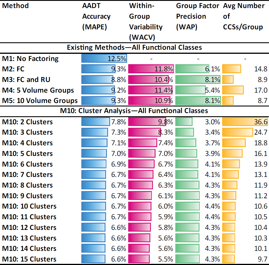
Table 4 shows the main aggregate results produced in NCHRP Project 07-30 from the validation of five traditional methods [M1: no factoring; M2: functional class (FC); M3: FC combined with rural/urban (RU) area type; M4: five volume groups (VGs); and M5: 10 VGs] and cluster analysis (M10). The latter involved running clustering multiple times by developing a different number of clusters each time. All methods were applied and validated using data from over 10,000 CCSs located in 45 states—three years per state. The validation was based on 24-hour sample counts taken from Monday through Friday.
This large validation dataset provided several benefits related to the extent and completeness of the analysis and the diversity in the results across the country; however, it was impractical to manually modify the thousands of factor groups generated by each method using localized knowledge of
Table 3. Strengths and weaknesses of cluster analysis.
| Strengths | Weaknesses |
|---|---|
|
|
Table 4. Performance metrics of existing traditional methods versus cluster analysis across all state-years examined in NCHRP 07-30.
 |
each of the 45 state transportation networks, as is typically done in practice, and recommended by federal guidance (FHWA 2022). In other words, the methods evaluated in NCHRP Project 07-30 relied solely on one or more grouping variables (e.g., functional class, area type, volume group) without applying knowledge of local patterns to identify recreational sites and potentially reassign CCSs to other factor groups based on unique regional factors. Therefore, the methods examined in NCHRP 07-30 represent “base” versions, and agencies can improve them (along with the produced results shown in the guide) if they apply local knowledge of their network to further refine the factor groups (M2–M5) or clusters (M10) created by each method.
The five columns in Table 4 show the method examined, the AADT accuracy (MAPE, Equation 18), the within-group variability (WACV, Equation 12), the group factor precision (WAP, Equation 15), and the average number of CCSs per group, respectively.
The results showed that regardless of the number of clusters created, cluster analysis outperforms all traditional methods, yielding more accurate AADTs (i.e., lower MAPE), more homogeneous groups (i.e., lower WACV), and more precise group factors (i.e., lower WAP). The improvement in AADT accuracy (i.e., decrease in MAPE) is more pronounced when the first few (3–7) clusters are created. Beyond a critical point, creating more clusters marginally improves the AADT accuracy, but the within-group variability (WACV) continues to decrease. Unlike the MAPE and the WACV, which exhibit decreasing trends as more clusters are created, the group factor precision (WAP) follows an increasing trend up to a certain point, beyond which it stabilizes. In general, the precision is disproportionally affected by the number of CCSs per cluster, which is in the denominator of the precision equation (Equation 13), but proportionally influenced by the variability (i.e., CV) of group adjustment factors, included in the numerator of the precision
calculation. When more clusters are created, CCSs are moved from old clusters to new clusters. As a result, both the average number of CCSs per cluster and the CV decrease. However, the reduction in the average number of CCSs per cluster is more significant compared to the reduction in the CV and, therefore, has a greater impact on the precision.
The general increasing/decreasing trends described above are observed in most states and years. One variable that can change from one state to another is the total number of CCSs within each state. This number affects the position of the critical point beyond which the AADT accuracy (i.e., MAPE) tends to stabilize or change at a very low rate. For example, Figure 5a shows the average performance metrics calculated for Vermont using data from 32 CCSs per year, whereas,
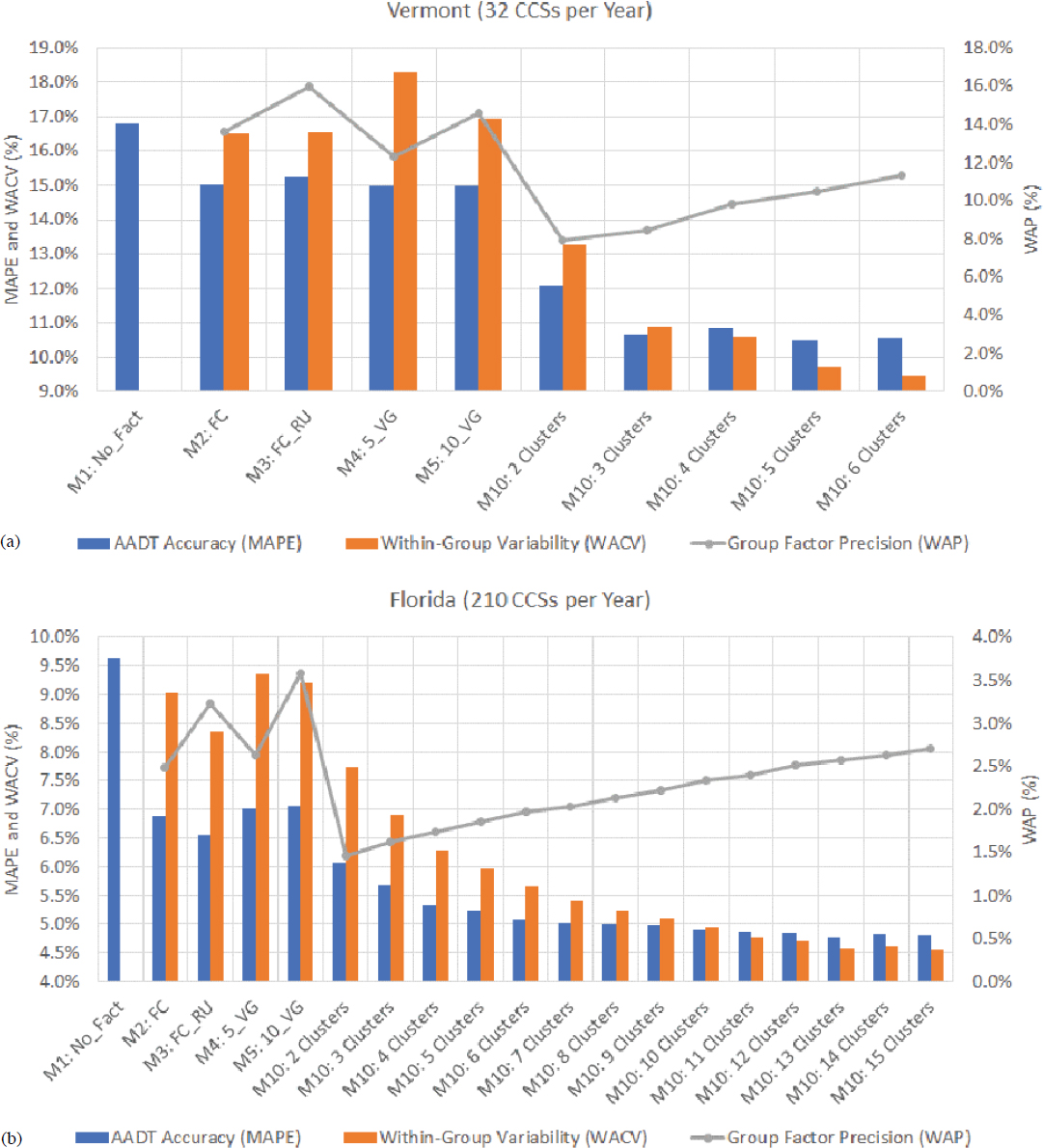
in Figure 5b, the performance metrics are based on 210 CCSs per year in Florida. In the case of Vermont, the MAPE stabilizes when three clusters are created, but in Florida, the MAPE continues to decrease at a very low rate as more clusters are developed.
Despite its superior performance over other simpler traditional methods, clustering has a few practical disadvantages. Its main shortcoming is that it may not be easy to define the produced clusters based on one or more distinct traffic, roadway, or other characteristics. As a result, assigning SDCs to the most suitable cluster may be a challenging task. This may also create difficulties in explaining clusters to other users. One option to partially overcome this challenge is to use the k-prototypes algorithm or hierarchical clustering that can handle both continuous variables (e.g., temporal adjustment factors) and categorical variables (e.g., functional class, area type, land use, etc.). More information on these methods is provided in subsequent sections in this chapter. Also, Appendix D provides examples of how to apply the k-prototypes algorithm in the programming language R using continuous and categorical variables.
No clustering algorithm or set of clustering inputs can automatically generate well-defined clusters. To address this need, the clusters generated by a computer need to be refined by applying engineering judgment and knowledge of the local transportation network. A second option to assign counts to clusters is to use a statistical or machine learning assignment method such as decision trees. More information about these methods is provided in the last section of this chapter, “Complementary Assignment Methods.”
Another major limitation of clustering is the lack of guidelines for determining the optimal number of clusters created by partitioning clustering methods, where users need to specify a priori the number of clusters to be produced. While mathematically, this is feasible by employing clustering optimization criteria (e.g., the pseudo-F statistic, elbow criterion, Bayesian information criterion, Akaike information criterion), the latter primarily account for changes in the within-group variability—not the AADT accuracy—as the number of clusters increases. This is problematic because, as explained above, the AADT accuracy starts to plateau before the within-group variability starts to decrease at a low rate.
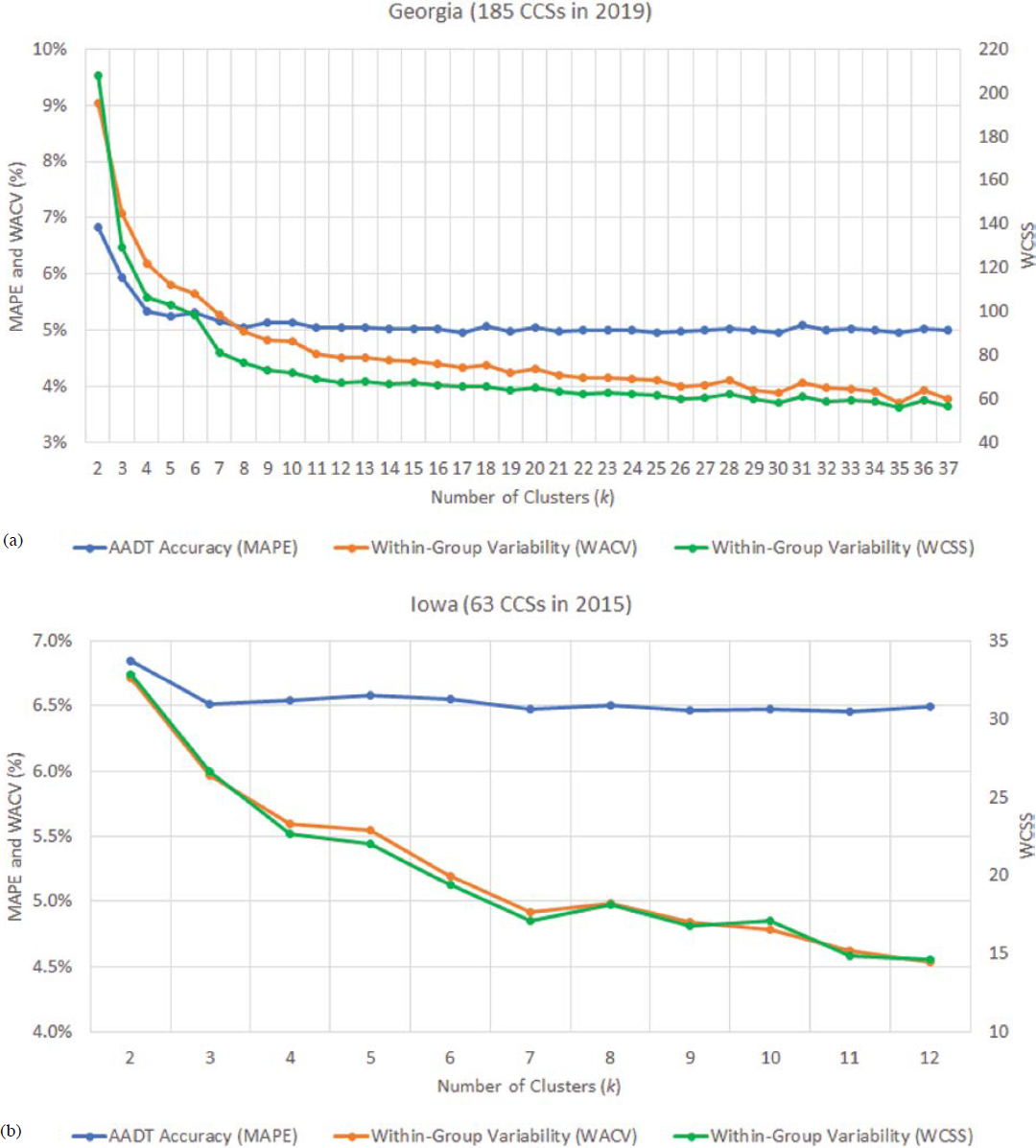
Figures 6a and 6b show graphs developed using data from Georgia and Iowa, respectively. In these graphs, both the WACV and the within-cluster sum of squares (WCSS) are measures of the within-group variability. The WCSS is computed in the elbow optimization criterion. Both the WCSS and the WACV exhibit similar decreasing trends as the number of clusters increases. Similar trends are consistently observed in many states and years. A common finding is that both the WCSS and the WACV continue to decrease even after the critical point beyond which the MAPE starts to plateau.
For instance, in Figure 6a, the MAPE stabilizes after creating four (k = 4) clusters, but the WACV and the WCSS continue to decrease at a relatively high rate until k = 11, after which their reduction rate significantly drops. In Figure 6b, no improvement in AADT accuracy is gained after creating more than three clusters, despite the fact that the within-group variability continues to decrease until the maximum number (max k = 12) of clusters is reached. The advantage of the WACV over the WCSS is that the former is expressed as a percentage, similar to the MAPE, making the visualization and interpretation of the results easier. Appendix B describes a case study in which Washington State Department of Transportation (WSDOT) used the WCSS to determine the optimal number of clusters.
In NCHRP 07-30, the pseudo-F statistic was also employed to automatically determine the optimal number of clusters by state and year. The results indicated that the optimal number of clusters in all 135 state-years examined in the project was 3.0; however, in many cases, the AADT accuracy continued to improve when more than three clusters were created, particularly when the number of CCSs was high.
Further, existing optimization criteria do not provide the flexibility to incorporate guidelines or other user preferences and constraints. As a result, engineering judgment is necessary to select a rational number of clusters and then make additional modifications if needed.
Like many statistical methods, clustering is also sensitive to outliers. The latter may affect the formation and the size of the clusters. Analysts should ideally identify and exclude potential outliers before performing clustering. One way to address this need is to calculate 12 monthly CVs (CV = standard deviation ÷ mean) for each CCS using the corresponding monthly adjustment factor from multiple years. For example, Figure 7 shows the monthly factors from 2016 through
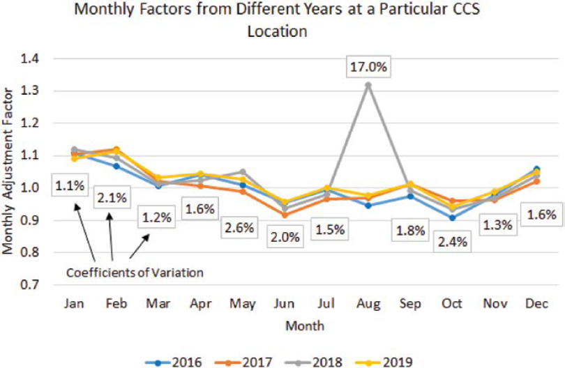
2019 at a particular CCS location. The percentages in rectangles are the 12 monthly CVs. Each CV was calculated using the four monthly adjustment factors from the four years (2016–2019) shown in the graph.
Though exceptions may occur, typical monthly CV values at nonrecreational sites are relatively small, usually less than 5 percent. Any CV greater than 5 percent should be further investigated to determine the reasons behind the high traffic variability within that month. High CV values may be indicators of possible outliers that should be removed. For example, in Figure 7, the CV for the month of August is 17 percent, whereas the remaining 11 CVs range from 1.1 percent to 2.6 percent. If similar graphs are constructed by including factors from all recreational and nonrecreational sites, high CV values may indicate the existence of either outliers (e.g., due to construction) or recreational traffic. In this case, local knowledge of the network should be used to investigate the reasons behind the atypical patterns. Potential outliers should be excluded, whereas recreational sites need to be kept but reassigned to a “recreational” factor group.
Another limitation of clustering is that the clusters tend to be unstable from one year to the next, complicating the development of factor groups (Faghri et al. 1996, Zhao et al. 2004). Agencies should ideally perform clustering every year to determine if new traffic patterns have emerged and make appropriate changes in the factor groups if needed. An alternative is to perform clustering using data from multiple (e.g., three) consecutive years. However, this option may lead to misleading results in case of potential changes in traffic patterns at one or more permanent sites due to new developments, construction, changes in land use, and others.
Also, cluster analysis may not be applicable to lower functional classes where only a few or no CCSs may exist in each state. To put things in perspective, the average number of CCSs on the three lowest roadway functional classes [rural minor collectors (6R), rural local roads (7R), and urban local roads (7U)] is 1.6 CCSs per state (Tsapakis et al. 2020, Tsapakis et al. 2021).
Clustering Types
The literature reveals a plethora of traditional and new clustering algorithms that have been used in various fields. For example, a 2015 survey of clustering algorithms identified nine groups
of traditional clustering algorithms and ten groups of modern algorithms (Xu and Tian 2015). The traditional algorithms are categorized based on partition, hierarchy, fuzzy theory, distribution, density, graph theory, grid, model, and fractal theory. The modern algorithms are based on kernel, ensemble, swarm intelligence, spectral graph theory, affinity propagation, density and distance, spatial data, data stream, large-scale data, and quantum theory. Each group contains multiple algorithms, and some algorithms may fall into one or more groups. More information about the different types of clustering algorithms is provided in the study by Xu and Tian (2015).
The clustering algorithms mainly differ in the following ways:
- the types of data (e.g., quantitative or qualitative variables) that each algorithm is designed for,
- whether similarities or dissimilarities between objects are calculated,
- the metrics used to capture similarities or dissimilarities, and
- how the objects are initially grouped.
Due to these differences, it is not easy to divide the various types of algorithms into a small number of distinct categories.
The clustering methods that have been used most frequently in the development of adjustment factor groups and are available in many statistical programs include non-hierarchical or partitioning clustering (Garber and Bayat-Mokhtari 1986, Flaherty 1993, Schneider and Tsapakis 2009, Tsapakis 2009, Tsapakis et al. 2011a, Tsapakis et al. 2011b, Gecchele et al. 2011, Rossi et al. 2014, Krile et al. 2015, Sfyridis and Agnolucci 2020) and hierarchical clustering (Sharma and Allipuram 1993, Sharma and Leng 1994, Sharma et al. 2000, Zhao et al. 2004). Some studies have also explored other clustering methods, such as model-based clustering (Zhao et al. 2004, Li et al. 2006, Gecchele et al. 2011, Rossi et al. 2014). However, the latter tend to be more complex and difficult to comprehend without providing a significant improvement in performance over other simpler methods. The following two sections present non-hierarchical and hierarchical methods, respectively. Each section discusses their main strengths, weaknesses, assumptions, and data considerations and provides suggestions for addressing some of their shortcomings.
Non-Hierarchical Clustering
Non-hierarchical or partitioning clustering creates non-overlapping partitions or clusters of objects, with each object belonging to one group (Aldenderfer and Blashfield 1984). A key characteristic of partitioning clustering is that users have to specify the number (k) of clusters to be developed. The clusters are created simultaneously and, therefore, do not have a hierarchical (e.g., tree-shaped) structure. The optimal number of clusters is unknown, particularly when new factor groups need to be created. For this reason, clustering is often performed multiple times by specifying a different number k of clusters each time, as shown in the previous section.
For example, it is common to initially create two clusters (k = 2) and sequentially increase the value of k by one up to a maximum value that should be less than the number of available CCSs within a state. To reduce computational time and the amount of effort required to review a large set of clustering results, the max k can be set equal to the total number of CCSs divided by a factor of two or three. This usually excludes clusters that contain a single CCS. A general recommendation is that each group of nonrecreational sites exhibiting moderately stable traffic patterns should have a minimum of six CCSs (FHWA 2022) so that the group adjustment factors meet the precision targets described in the previous chapter. Therefore, small clusters containing one or two CCSs are usually not desired unless the CCSs are located on recreational roads or the objective of clustering is to determine locations with unusual patterns that do not fit in any group.
The partitioning algorithm initially assigns each CCS to one of the predefined k groups, and then at each step of the process, each CCS is moved to the most similar cluster based on a similarity distance/metric. Depending on the clustering algorithm used, the goal is to maximize the similarity
or minimize the dissimilarity within each cluster while maximizing dissimilarity between clusters. This is achieved by optimizing an objective function, such as minimizing the intra-cluster variance and maximizing the inter-cluster variance. The k-means and the k-prototypes clustering algorithms are described below.
K-Means Algorithm
K-means is one of the most popular partitioning algorithms. It can handle continuous variables such as adjustment factors. It starts with the determination of cluster centers or centroids, which can be designated by the user or constructed automatically by the algorithm. In the next step, each CCS is assigned to the nearest cluster based on a distance/metric (e.g., the Euclidean distance computes the sum of squared distances between objects and cluster centroids). After the first assignment of all CCSs to clusters, all cluster centroids are recalculated based on the mean values of the objects in each cluster. These steps are repeated until any reassignment of CCSs does not change the value of the cluster centers by a certain threshold, known as the convergence criterion, or the maximum number of iterations set by the user is reached. Table 5 summarizes the strengths and weaknesses of the algorithm.
The k-means algorithm is relatively simple compared to other, more advanced algorithms. It is efficient and can not only handle large datasets that may contain a high number of CCSs but also work with a large number of independent variables and records. Many software packages provide various outputs, such as the cluster membership of each CCS at every iteration, the distance from cluster centers, analysis of variance results, and other statistics that capture the contribution of each variable to the separation of the clusters.
On the other hand, the algorithm is designed for continuous variables that ideally should be of the same scale. If continuous variables measured in different scales are to be used (e.g., adjustment factors, traffic volumes, and geographic coordinates), users should consider normalizing the variables first using an appropriate method such as the min-max scaling equation (Jin et al. 2008):
| (20) |
Where:
Xscaled = scaled variable.
X = original variable.
min(X) = minimum value of original variable.
max(X) = maximum value of original variable.
The normalization ensures that all variables contribute equally to clustering, regardless of their original scales.
As explained previously, another shortcoming of all partitioning algorithms is the need to specify the number (k) of clusters beforehand. The k-means algorithm is also sensitive to the initial
Table 5. Strengths and weaknesses of k-means algorithm.
| Strengths | Weaknesses |
|---|---|
|
|
determination of centroids. Different initializations may yield different final clusters. The algorithm is also sensitive to outliers since the latter may affect the centroids and the final size of clusters.
K-Prototypes Algorithm
The k-prototypes algorithm is a combination of the k-means and the k-modes algorithms (Sfyridis and Agnolucci 2020). It can develop clusters using both continuous variables (e.g., adjustment factors, traffic volumes, etc.) and categorical variables (e.g., functional class, rural/ urban area type, land use, etc.). The cluster development process using k-prototypes is similar to that of the k-means algorithm described above. The main difference is that each object is assigned to the nearest cluster based on not only distances computed using numerical data (e.g., Euclidean distance) but also other distances suitable for categorical features (Huang 1998). Distances/metrics that are commonly used to measure dissimilarity between data points of categorical variables are the simple matching coefficient, the hamming distance, and the Jaccard similarity coefficient. These distances/metrics are automatically computed by the software that executes the k-prototypes clustering. Understanding the calculation of the metrics and the software may be helpful, but it is not required to interpret the clustering results.
Appendix D provides an example of performing k-prototypes clustering in R, an open-source programming language, using as inputs 12 monthly adjustment factors and the roadway functional class combined with the rural/urban area type of each CCS. Similar to the k-means algorithm, if the continuous variables are of different scales, they need to be normalized, as explained above. With a few exceptions, the k-prototypes algorithm has similar strengths and weaknesses (see Table 6) as the k-means algorithm.
Because it can handle mixed variable types, the k-prototypes algorithm can potentially produce more well-defined clusters than the k-means algorithm. The clusters produced by k-prototypes can exhibit similar traffic patterns (e.g., using temporal adjustment factors) and also share other common qualitative characteristics (e.g., functional class) that can potentially facilitate the assignment process.
There is a tradeoff between using only numerical variables and combining them with categorical variables. As more qualitative variables are combined with numerical variables, the definition of clusters improves, but the within-cluster variability increases. The reduced internal homogeneity of the clusters tends to slightly reduce the accuracy of the AADT estimates derived from factored counts.
One disadvantage of k-prototypes is that it does not provide variable importance scores or statistics like other machine learning methods do; however, many software packages provide users with the option to specify the weight assigned to each numerical and categorical variable that is used as input to develop clusters. As the weight of the categorical variable(s) increases, the development of the clusters relies more on these (categorical) variables, improving the definition of the produced clusters but making them internally more variable. For this reason, it is common
Table 6. Strengths and weaknesses of k-prototypes algorithm.
| Strengths | Weaknesses |
|---|---|
|
|
to initially develop clusters using only numerical variables to determine if one or more clusters share some assignment characteristics.
The most important continuous clustering variables are the 84 monthly day-of-week factors and the 12 monthly factors of each CCS. Additionally, incorporating the geographic coordinates of CCSs into clustering can assist in grouping sites that have similar patterns and are also located close to each other (Zhao et al. 2004). If the produced clusters are poorly defined, qualitative variables may be included in the model by initially assigning low weights to them. For example, a starting point is to assign 10 percent to qualitative variables and 90 percent to numerical variables. The roadway functional class, the area type (e.g., rural and urban), and land use characteristics (if available) are the most important qualitative variables that can potentially improve the definition of clusters (Regehr et al. 2015, Sfyridis and Agnolucci 2020). However, the influence/ importance of each of these variables in the grouping process varies geographically by state and region. Users may need to perform clustering a few times by increasing the weights assigned to the categorical variables each time until the clusters are better defined.
Hierarchical Clustering
Hierarchical clustering groups objects in a tree-shaped structure, known as a dendrogram. Dendrograms provide a visual representation of the relationships among clusters. There are two types of hierarchical clustering: agglomerative and divisive.
Agglomerative clustering initially assigns each object to a single group. At each step of the clustering process, the two most similar groups are merged into a new group based on a linkage method and a similarity distance/metric. The linkage method dictates how the distance between existing clusters is calculated during the merging process, while the distance/metric measures the dissimilarity between individual objects. Common types of linkage methods include single linkage, complete linkage, average linkage, and Ward’s Method. Commonly used distances/metrics are the Euclidean distance, the Manhattan distance, and the correlation distance. This merging process is repeated until all objects are grouped into a single cluster.
On the other hand, in divisive hierarchical clustering, all objects are initially grouped into a single cluster. Pairwise dissimilarities between objects are computed in the next step, and the cluster is split into two subclusters that are least similar. The splitting process is repeated multiple times until each object is in its own cluster.
Figure 8 displays an example dendrogram of CCS clusters created using agglomerative clustering. Each leaf node along the vertical axis at the left of the dendrogram corresponds to one of the 20 CCSs clustered in this dendrogram. Internal nodes represent merged clusters at different levels of similarity. The horizontal axis shows the distance among clusters when they are merged.
To obtain a specific number of clusters, users must make a cross-section cut at a particular point on the dendrogram. For example, in the dendrogram shown in Figure 8, a cut needs to be made vertically. The resulting clusters align with the branches at the cutting point. For instance, if a cut is made between distances 20 and 25, the CCSs would be divided into two clusters. A cut at distance 5 yields five clusters.
Table 7 summarizes the strengths and weaknesses of hierarchical clustering. One difference between hierarchical clustering and other clustering methods is that the dendrograms produced provide a visual, intuitive representation of the relationships among clusters. Users can develop a better understanding of the data by reviewing how the various subclusters created during the merging process are interconnected.
Additionally, hierarchical clustering computes all possible pairwise distances among objects (i.e., CCSs) during the merging process. Consequently, it is not sensitive to how the initial clusters are constructed. Unlike other methods, hierarchical clustering does not assume equal cluster sizes, making it well-suited for datasets with varying cluster densities.

Further, some statistical software and programming languages (e.g., R, Python) can handle mixed data types. For example, the “hclust” function in R can handle mixed data types using the “daisy” function from the “cluster” package, which supports various distance metrics for both continuous and categorical variables. Figure 9 shows an example of performing hierarchical clustering in the programming language R using both continuous and categorical variables.
On the other hand, hierarchical clustering comes with certain limitations, particularly when applied to large datasets. One notable drawback is that it is not recommended for datasets containing a high number of CCSs (e.g., >100). The algorithm tends to become computationally intensive
Table 7. Strengths and weaknesses of hierarchical clustering.
| Strengths | Weaknesses |
|---|---|
|
|

and time-consuming in such scenarios, impacting its efficiency and scalability. The challenges further extend to the review process, especially when dealing with large dendrograms constructed using many CCSs. Navigating and interpreting extensive dendrograms can be a complex and demanding task.
Additionally, hierarchical clustering requires users to select the optimal number of clusters. This step introduces a level of subjectivity into the process since there is no standardized or objective criterion for determining the ideal number of clusters. Consequently, the choice may vary based on individual preferences and perspectives.
Another limitation is the algorithm’s sensitivity to outliers, which may influence the final clusters. Outliers in the dataset can distort the hierarchical tree structure, leading to the formation of clusters that are disproportionately affected by extreme values. As a result, users need to be cautious and consider preprocessing steps when dealing with datasets that may contain outliers.
Complementary Assignment Methods
As previously explained, users should ideally develop clusters and then make necessary refinements so that the final factor groups are clearly defined from a practical standpoint. This clarity is important for effectively assigning counts to factor groups based on one or more easily identifiable assignment characteristics. In practice, developing well-defined clusters may be a challenging and time-consuming task that involves several steps. For example, analysts usually have to:
- Map the CCSs of each cluster.
- Plot and visually examine their traffic patterns.
- Identify potentially common characteristics (e.g., FC, RU, land use, region, etc.) of the CCSs within each cluster.
- Determine the CCSs that can remain in a cluster and those that need to be reassigned to other groups.
- Calculate the precision of group adjustment factors for each modified cluster to meet relevant (precision) targets.
- Determine the required sample size of each group.
During this process, some clusters may exhibit distinct seasonal and time-of-day traffic patterns that may be worth keeping as separate factor groups. Nevertheless, the CCSs of these clusters may not have any unique characteristics upon which a cluster can be explicitly defined. Dissolving poorly defined clusters by reassigning their CCSs to other potentially better-defined clusters could increase the within-group variability and decrease the effectiveness of the remaining clusters.
Appendix A describes a unique statistically based assignment approach that the North Carolina Department of Transportation (NCDOT) uses to assign seasonal counts to six factor groups. In brief, NCDOT conducts four four-day counts per year at each count location. An AADT estimate is obtained by annualizing the four seasonal counts taken at each location using appropriate adjustment factors from every factor group. The result is 120 AADT estimates (= 4 seasonal counts × 5 days per count × 6 factor groups) per count location and year. NCDOT calculates the CV of the 20 AADT estimates (= 4 seasonal counts × 5 days per count) generated for each group. In the last step, the count is assigned to the factor group that results in the lowest CV. As described in Chapter 4, this approach can also be used to evaluate whether an SDC station has been assigned to the appropriate factor group even if the assignment was originally performed using a different method (e.g., functional classification).
Another option is to employ machine learning methods to assign counts to poorly defined clusters, which nonetheless may have unique traffic patterns. The assignment can be performed in a data-driven manner based on common attributes that can be determined for both clusters and counts. Table 8 briefly describes various machine learning methods that can be used for classification purposes (Gecchele et al. 2012, Rossi et al. 2012, Tsapakis and Schneider 2015), and Table 9 summarizes their strengths and weaknesses (Murphy 2012, Shalev-Shwartz 2014).
Table 8. Machine learning methods suitable for assignment purposes.
| Method | Description |
|---|---|
| Artificial neural networks | A collection of input, hidden, and output layers of interconnected neurons. Each neuron produces an output, which then becomes the input to the next layer. This continues until the terminal neurons produce an output. |
| Decision tree | A tree-shaped model that continuously splits the dataset into subsets based on one attribute at each split. The splitting process terminates when certain criteria are met. |
| Discriminant analysis | A model that finds linear combinations of common assignment characteristics between SDCs and factor groups and calculates the probability of group membership for each SDC. |
| Random forest | Random forest constructs multiple decision trees from randomly selected subsets of the entire dataset. It can be used for classification and prediction. In the case of classification, the SDC is assigned to the CCS selected by most trees. In the case of prediction, the output is the average of all values predicted by the trees. |
| Gradient boosting | Unlike random forests that build several independent trees at once, gradient boosting starts by building a collection or ensemble of “weaker” trees and then iteratively and sequentially learns from each weak tree to build a stronger model. It can be used for prediction, classification, and ranking. |
| K-nearest neighbors | A method that can be used for classification and regression. It identifies the k most similar CCSs that are closer to an SDC. In the case of classification, the SDC is classified by a plurality vote of its neighboring CCSs and is assigned to its most similar CCS based on certain characteristics. The output is a class membership. In the case of regression, the output is a property value, which is the average of the values produced by the algorithm. |
| Support vector machine | A method that uses a kernel function to transform nonlinearly separated data from an input space to a feature space where data are linearly separated and then are transformed back to the input space, where they again become nonlinear. |
Table 9. Strengths and weaknesses of various machine learning methods.
| Method | Strengths | Weaknesses |
|---|---|---|
| Artificial neural networks |
|
|
| Decision trees |
|
|
| Discriminant analysis |
|
|
| Gradient boosting |
|
|
| K-nearest neighbors |
|
|
| Random forest |
|
|
| Support vector machines |
|
|
The effectiveness of these methods is greater when the number of clusters to which counts can be assigned is small and when each cluster has unique traffic patterns. The methods are not needed if the factor groups are well-defined. Though the performance of these methods is generally satisfactory, the methods tend to have complicated structure, and decreased interpretability, and there is limited reproducibility of the results. For these reasons, the methods are often called “black boxes.” Some of them operate in complex, nonlinear ways that are challenging for humans to fully understand. Some methods produce different results every time they are trained or evaluated because of the randomness and stochastic nature of their algorithms.
NCHRP Project 07-30 validated several decision trees and support vector machines and found that the latter performed slightly better than the decision trees. However, the decision trees’ simplicity and intuitiveness outweigh the marginal performance gains obtained from the more complex support vector machines. Due to the complexity and implementation considerations associated with many machine learning methods, the next section presents decision trees, which are easier to understand, apply, and interpret compared to other methods.
Decision Trees
Decision trees were introduced in 1984 by Breiman et al. They are a machine learning method widely used for regression and classification tasks, including assigning objects to groups. For the purposes of this guide, the goal of decision trees is to predict the cluster membership of a count based on a set of independent variables (e.g., hourly factors, functional class, area type, etc.) that are common between a count and each cluster.
A decision tree is a vertical or horizontal flowchart that includes nodes connected with branches. Figure 10 shows the main components of a tree. The first (root) node in a tree is split into two internal nodes based on a decision rule that relies on an independent variable. Among all independent variables used to construct a tree, the algorithm determines the variable and the split point that provides the best separation of the dataset into different classes or groups. This is done using an impurity measure that assesses the homogeneity of a node. If a node is highly variable or impure, it will be split into two more homogeneous nodes. For example, a decision rule can be “is functional class 1 or 2?” Another example of a rule that a continuous variable can be is “Is the 10th hourly factor on a Monday in January greater than 10.0?”

Each of the two internal nodes may be further split into new nodes based on a new decision rule. The splitting process is repeated until a predetermined stopping criterion is met. The nodes that are not split further are the terminal or leaf nodes of the tree (Figure 10). The tree predicts a target value (i.e., cluster membership) for each terminal node.
To develop a tree, analysts need to prepare a training set using data from the CCSs that belong to the clusters of interest. The training set should contain independent variables that can also be calculated from SDCs. Examples of important independent variables that are common between clusters and counts include continuous variables (e.g., hourly factors by day of year, hourly factors by month and day of week) and categorical variables (e.g., functional class, area type, land use).
Once a decision tree is trained, it can be applied to assign new counts not included in the training set to the clusters of interest. The new counts need to be included in a testing test, which is fed into the tree. The latter automatically checks whether the new counts meet the decision rules at each node of the tree starting from the root node. If the decision rule at the root node is met (i.e., the answer to the rule/question is yes), the algorithm proceeds to the left branch checking the decision rule at the first internal node downstream. If a rule is not met (i.e., the answer to the rule/question is no), the algorithm follows the right branch and checks the validity of the rule at the next node downstream. This process is repeated until a terminal node is reached, which indicates the cluster membership of the count.
Statistical programs typically output decision trees as diagrams or tables containing each node’s decision rule. Some of them provide statistics that capture the improvement achieved when a node is split and the importance of each independent variable. The importance of a variable depends on all the improvements observed in the nodes that were divided based on that variable.
Decision trees have several advantages related to the data that they can handle. Unlike some statistical models, decision trees make no assumptions about the underlying distribution of the data. This flexibility allows them to handle both continuous and categorical variables. Further, they are not sensitive to the scale of input variables, eliminating the need for data normalization or scaling. This makes them suitable for datasets with heterogeneous scales. Decision trees can automatically select relevant attributes for decision-making. This feature simplifies the process of identifying key variables that contribute to the model’s accuracy by ignoring unimportant features that have minimal impact on the model’s performance. Decision trees can also use the same variable multiple times in a tree, allowing them to capture complex interdependencies among variables. In addition, they are less influenced by outliers compared to other machine learning algorithms. Outliers may affect individual branches but are less likely to distort the overall model.
Despite their flexibility in handling mixed data types, decision trees have some limitations. They are prone to overfitting, especially when the model becomes too complex and closely fits the training data. Small changes in the training dataset, such as the addition or removal of data points, can lead to different tree structures. This sensitivity may impact the model’s stability. Further, large decision trees can be challenging to interpret and present. Communicating the logic of complex structures to non-experts may require simplification or additional visualization aids. Decision trees may be sensitive to the choice of some parameters, such as tree depth, minimum impurity decrease to split a node, and the minimum number of objects within each terminal node.


