Guide on Methods for Assigning Counts to Adjustment Factor Groups (2024)
Chapter: 5 Adjustment Factors Using Probe Data

CHAPTER 5
Adjustment Factors Using Probe Data
Introduction
This chapter describes how probe data from third-party vendors can be used to develop segment-specific adjustment factors and then annualize SDCs. The chapter includes three sections that provide information related to the following topics that the research team aimed to examine in relation to probe data:
- Development of adjustment factors from probe data.
- Accuracy of AADT estimates derived from counts annualized using probe-based factors.
- Applicability of probe-based factors to lower functional classes.
What Are Probe Data?
Probe data include timestamped location data collected from various sources, including but not limited to phones, tablets, portable global positioning system (GPS) devices, GPS devices embedded in vehicles, smartphone applications, other mobile devices, and connected and autonomous vehicles. The probe data are captured at a certain sample frequency (e.g., every three seconds). Probe data typically capture only a sample of vehicles (or “probes”) of the entire vehicle population in the traffic stream. The ratio of the total number of probes to the total number of vehicles at a particular location and within a certain period represents the penetration rate of a raw probe dataset for that period.
Probe data can be used to estimate various traffic parameters, including, but not limited to, speed, travel time, origin-destination tables, and volume. Probe data are sold by a number of third-party data vendors. Many vendors obtain various types of probe data from different sources and then use advanced machine learning methods such as random forests, gradient boosting, and artificial neural networks to develop their products (Schewel et al. 2021). The vendors typically do not disclose their data sources and processing algorithms.
The two most common data sources are location-based services and connected vehicles. Location-based service (LBS) data come from mobile devices such as smartphones, which use a combination of GPS, Wi-Fi, Bluetooth, and cell tower signals to determine the device’s location. Device locations are collected at regular intervals by wireless carriers and by many smartphone application developers. These companies then sell LBS data to third-party data vendors. Connected vehicle data come from vehicle systems and on-board devices. Most newer passenger cars have GPS receivers and cellular connections for their navigation, entertainment, and security systems. Trucks have GPS and cellular or Bluetooth communications in their electronic logging devices (ELDs), and newer models may also have vehicle systems similar to those found in passenger cars. Vehicle locations and other attributes are collected at regular intervals by vehicle and ELD manufacturers, who may sell connected vehicle data to third-party data vendors.
Several data processing steps are applied by third-party data vendors to prepare location data for transportation applications. A key processing step for all location data is map matching, where the location points from a particular trip of a probe device are used to determine the most probable route taken through the road network. Map matching methods use knowledge of the roadway network and trip-specific attributes, like speed and travel time, to distinguish between similar routes. LBS data may include both motorized and nonmotorized trips. Machine learning models can be trained to classify trips by mode based on characteristics such as speed, travel time, and route. Vendors may apply additional processing steps to remove duplicate trip records (which can occur when multiple devices travel in the same vehicle) and to produce estimates such as total volume from the probe sample.
Strengths and Weaknesses
Annualizing SDCs using probe-based, segment-specific temporal adjustment factors is a promising assignment method primarily due to the continuously increasing penetration of probe data in the traffic stream. Table 13 summarizes the strengths and weaknesses of probe-based adjustment factors. Probe factors can potentially be developed for every roadway segment of the transportation network, even those on lower functional classes. This granularity enables a more detailed understanding of traffic patterns, including those on recreational roads, across the entire road network.
Probe factors eliminate the need to develop adjustment factor groups and assign counts to them. This streamlines the AADT estimation process, saving time and resources while eliminating the errors associated with these intermediary steps. The simplicity and directness of probe-based adjustment factors make them easy to explain to a diverse audience. This is important for effective communication with stakeholders, decision-makers, and other end users who may not be familiar with the intricacies of traffic analysis.
While probe-based adjustment factors offer several advantages, they have a few limitations. One consideration is that the accuracy of these factors heavily relies on the penetration rate of probe data and how well the probe samples represent the entire vehicle population. A low penetration rate or biased representation of the overall traffic flow may compromise the effectiveness of the adjustment factors. For example, LBS data from smartphone applications may exhibit higher penetration rates in dense urban areas around shopping centers compared to rural areas. Connected vehicle data
Table 13. Strengths and weaknesses of probe-based adjustment factors.
| Strengths | Weaknesses |
|---|---|
|
|
from a limited number of original equipment manufacturers (OEMs) may not be representative of the entire traffic flow, especially on routes dominated by truck traffic. Oversampling can also be an issue, particularly when multiple probe devices (e.g., smartphones) are present in a single vehicle.
The dynamic nature of probe data may also introduce challenges. The addition of new probe data sources to existing datasets from a vendor can lead to abrupt changes in temporal traffic patterns, impacting the accuracy of adjustment factors. Similarly, discontinuation of one or more probe data sources may cause sudden shifts in patterns, affecting the effectiveness of probe factors.
Another drawback is the limited availability of probe data for higher vehicle classes, such as trucks. This limitation can hinder the development of truck-specific temporal adjustment and axle-correction factors, especially when trying to account for the diverse characteristics of various vehicle types.
Furthermore, storing and processing large volumes of raw probe data demands advanced computer hardware and software capabilities. This can pose challenges for transportation agencies that may have limited technical expertise, technological infrastructure, and cloud storage and computing resources required to handle big data. In practice, transportation agencies often purchase processed aggregated probe-based products from private vendors, who typically manage and process raw probe “big” data. Though this may alleviate the challenges associated with managing extensive datasets, including handling personally identifiable information, it limits agencies’ ability to fully understand the characteristics and potential biases inherent in the data.
FHWA pooled-fund study TPF-5(384) developed guidelines for obtaining AADT estimates from nontraditional sources (Hallenbeck et al. 2021). The document discussed how transportation agencies can purchase or accept probe-based traffic volume estimates from data vendors. Further, Chapter 6 of the 2022 TMG provides information on third-party data needs, quality, ownership, management, rights, version control, and costs (FHWA 2022).
Probe-Based Factors
The results produced in NCHRP 07-30 indicate that probe data can be a viable data source for calculating temporal adjustment factors. However, as of the publication of this guide, it is more difficult to develop axle-correction factors due to the limited availability of probe data for specific vehicle classes. In general, the effectiveness of probe-based factors in annualizing counts depends on several interconnected factors, of which the most important are:
- The penetration rate of the raw probe data.
- The types of probe data (e.g., GPS, LBS, connected vehicles) and their representativeness of the entire vehicle population.
- The correlations between probe-based factors and actual adjustment factors.
- The types of adjustment factors being used.
Temporal Adjustment Factors
As described above, probe data capture a sample of the total traffic on a given roadway segment. Provided that this sample is unbiased the raw probe trip counts on a roadway segment can be expected to follow the same monthly, day-of-week, and daily variations as the total volume on that segment. Similar to actual CCS volume data, probe trip data can be used to calculate various average probe counts and adjustment factors at a specific roadway location or segment for a given time interval:
- Average probe counts:
- 1 annual average daily probe count (AADPC).
- 7 annual average day-of-week probe counts (AADWPCs).
- 12 monthly average daily probe counts (MADPCs).
- 84 monthly average day-of-week probe counts (MADWPCs).
- 365 average daily probe counts (ADPCs).
- Probe-based adjustment factors:
- 7 annual day-of-week factors (= AADPC ÷ AADWPC).
- 12 monthly factors (= AADPC ÷ MADPC).
- 84 monthly day-of-week factors (= AADPC ÷ MADWPC).
- 365 daily factors (= AADPC ÷ ADPC).
The equation for calculating probe-based adjustment factors is the same as that using actual CCS volume data (Equation 7). The main difference is that in the numerator, the AADT is replaced by the AADPC, and in the denominator, the average traffic volume is replaced by the corresponding average probe count. To be able to calculate the AADPC, and thus the probe-based adjustment factors, probe data have to be available for at least 12 consecutive months.
Penetration Rate
The penetration rate of the probe data is not required for the calculations described above because the adjustment factor for a given time interval reflects the variation in traffic relative to the annual average. However, it is important to understand whether and how the penetration rate varies over time. As new sources of probe data emerge, vendors may incorporate new probe data into their databases to increase the penetration rate of their data and, therefore, the accuracy of their products. However, adding new sources of probe data to existing datasets may lead to sudden changes in temporal probe-based traffic patterns and, as a result, affect the accuracy of probe-based adjustment factors developed using existing data. Likewise, the discontinuation of one or more probe data sources may also affect the seasonal and day-of-week probe-based traffic patterns and the accuracy of adjustment factors and other probe-based products such as volumes. The penetration rate at a particular CCS location can be calculated as follows:
| (22) |
Where:
PRi = penetration rate of probe data at CCS i.
d = day of year (1, 2, . . ., 365 or 366 in leap years).
dmax = total number of days in a year (365 or 366 in leap years).
ADTd,i = average daily traffic at CCS i on day-of-year d.
ADPCd,i = average daily probe count at the location of CCS i on day-of-year d.
If some of the 365 or 366 ADT values of a CCS have missing data, the denominator in the equation above should be replaced by the AADT of CCS i multiplied by 365 or 366 days. The penetration rate can vary significantly from one vendor to another depending on the types and the number of probe datasets each vendor obtains from various sources (e.g., smartphone applications, connected vehicles, etc.). Though exceptions exist, the higher the penetration rate, the higher the correlation between probe-based factors and actual adjustment factors calculated from CCS data.
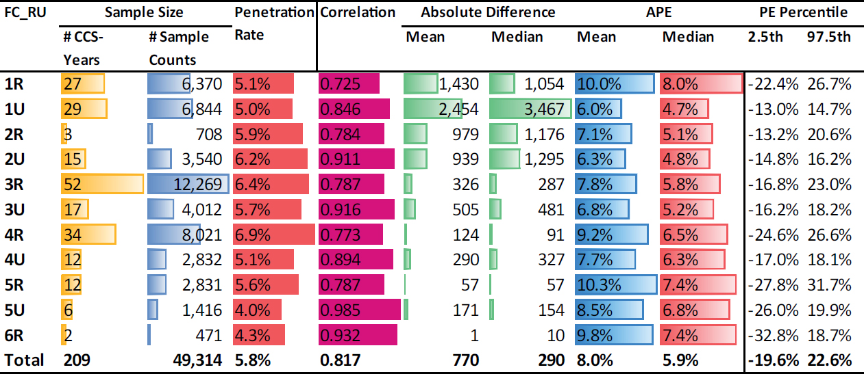
In NCHRP 07-30, probe datasets from three vendors and states were used to calculate probe-based adjustment factors at CCS locations. The quality of the probe-based adjustment factors was evaluated by comparing the correlations of the probe-based factors to the actual adjustment factors derived from CCSs. The correlations shown in Table 14 suggest that probe data can produce factors that are strongly correlated with actual adjustment factors given a sufficiently high penetration rate. The highest penetration rate was determined for Vendor A, which obtained
Table 14. Penetration rate of raw probe data and correlations of probe-based versus actual adjustment factors.
| Vendor (State) | Year | # CCS-Years | Average Penetration Rate | Correlations of Probe-Based vs. Actual Adjustment Factors | |||
|---|---|---|---|---|---|---|---|
| 7 Day of Week | 12 Monthly | 84 Monthly Day of Week | 365 Daily | ||||
| Vendor A (TX) | 2021–2022 | 209 | 5.83% | 0.817 | 0.788 | 0.795 | 0.844 |
| Vendor B (OH) | 4/1/2021–3/31/2022 | 46 | 0.39% | 0.549 | 0.509 | 0.399 | 0.311 |
| Vendor C (MN) | 2017–2019, 2021 | 97 | 2.86% | N/A | 0.325 | N/A | N/A |
connected vehicle data from several OEMs. The data of the other two vendors primarily included LBS data generated or collected from smartphones or other probe devices.
Probe trip counts may vary for reasons unrelated to traffic volumes, such as a change in the penetration rate of roadway users using location-based services or connected vehicles or a change in the vendor’s data sources. Transportation agencies or other end users of probe-based data products should request that data vendors track, document, and communicate such changes in their data stream because they can affect not only the accuracy of probe-based patterns and adjustment factors but also that of other probe-based data products.
Axle-Correction Factors
The research team also evaluated the accuracy of probe-based factors developed for two groups of vehicle classes: medium-duty (FHWA vehicle classes 4–6) and heavy-duty (FHWA classes 7–13) vehicles. The probe-based adjustment factors for these two vehicle groups were compared to actual adjustment factors calculated from vehicle classification CCS data. Table 15 shows the main results from this analysis.
The analysis revealed several issues with probe-based classification counts, indicating that probe data are not currently a mature and viable data source for calculating axle-correction factors. Probe-based classification data were challenging to obtain, with only one of the three vendors having aggregated probe trip counts for these two vehicle groups (i.e., not disaggregated by vehicle class). For axle correction, these groups are too coarse, as vehicle classes 7–13 vary significantly in the number of axles. Another issue was that raw probe trip counts were provided on a monthly basis and rounded to the nearest 1,000. This aggregation limited the temporal adjustment factors that could be calculated, and the rounding introduced significant errors since actual truck counts were fairly low at many CCS locations.
In general, it is difficult to develop temporal adjustment and axle-correction factors for specific truck types due to the limited availability of probe data for higher vehicle classes. However,
Table 15. Penetration rates and correlations of probe-based versus actual adjustment factors.
| Vendor (State) | Year | Truck Group | # CCS-Years | Average Penetration Rate | Correlation of Probe vs. Actual 12 Monthly Adj. Factors | MAPE |
|---|---|---|---|---|---|---|
| Vendor C (MN) | 2017–2019, 2021 | Medium-Duty Trucks | 44 | 27.7% | 0.312 | 42.6% |
| Heavy-Duty Trucks | 28.6% | 0.327 | 42.8% |
as more probe devices enter the traffic stream, the penetration rate of truck-specific probe data is expected to increase along with the accuracy of probe-based factors and other data products developed specifically for trucks.
Accuracy of AADT Estimates
The accuracy of AADT estimates developed from counts that have been annualized using probe-based temporal adjustment factors can be equivalent to or better than the accuracy of traditional methods, given a sufficient penetration rate of probe data. For example, the research team determined the accuracy of AADT estimates derived from SDCs factored using four sets of probe-based factors: 7 day-of-week factors (DWFs), 12 monthly factors (MFs), 84 MDWFs, and 365 DFs. This was separately done using temporal adjustment factors for all vehicles as one group, as well as for two groups of vehicle classes, medium- and heavy-duty trucks. The best results were obtained for the seven day-of-week factors.
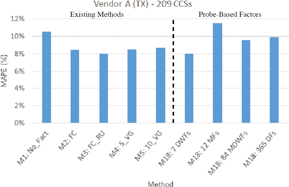
In Method 18 (M18), raw probe trip counts were used to calculate probe-based adjustment factors on roadway segments where CCSs were available. To determine the accuracy of AADT estimates, 24-hour sample counts were extracted from each CCS, factored with the appropriate probe-based adjustment factor, and compared to the actual AADT of the “parent” CCS. Figure 11 shows the MAPE of AADT estimates derived from sample counts annualized using the traditional methods (M1–M5) and four sets of probe-based adjustment factors developed for Texas (Vendor A).
The probe-based seven day-of-week factors produced the same MAPE as FC_RU (M3), and the resulting AADT estimates were more accurate than those of the other four methods. Vendor A had the highest penetration rate among all three vendors. Similar results were found for Vendor B, as shown in Figure 12, though the errors of the probe-based AADT estimates were higher due to the low penetration rate of Vendor B’s probe data. For this reason, the range of the y-axis (MAPE) in Figure 12 (0–60 percent) is much larger than that in Figure 11 (0–12 percent). The MAPE for the 12 monthly factors for Vendor C was 24.2 percent, which was significantly higher than all existing

methods, primarily due to the issues described above related to the penetration rate and the rounding of raw probe trip counts.
Table 16 shows the MAPEs obtained from the validation of probe-based factors developed for medium- and heavy-duty vehicles. The MAPEs in both vehicle groups were around 43 percent, significantly higher than those obtained from the probe-based factors for all vehicles. The rounding of raw probe trip counts partially explains the poor performance of these factors since the rounding error is proportionally larger at lower trip counts. However, AADT estimates for a subset of vehicle classes would be expected to have higher errors than those for all vehicles due to the smaller sample size of these subsets.
Lower Functional Classes
Another research question that NCHRP 07-30 aimed to address was whether probe-based adjustment factors can be used to factor counts taken on lower roadway functional classes. The research results generally support the use of probe-based adjustment factors on lower functional classes, although there is a trend of decreasing penetration rate and increasing AADT estimation errors when moving from higher to lower functional classes.
The seven day-of-week factor results from Vendor A were aggregated by FC and then by FC_RU to investigate trends. Table 17 shows the main results aggregated by FC. One finding is that the
Table 16. Penetration rates and correlations of probe-based versus actual adjustment factors (M19).
| Vendor (State) | Year | # CCS-Years | Vehicle Group | Average Penetration Rate | Correlation of Probe vs. Actual 12 Monthly Adjustment Factors | MAPE |
|---|---|---|---|---|---|---|
| Vendor C (MN) | 2017–2019, 2021 | 44 | Medium-Duty Vehicles | 27.7% | 0.312 | 42.6% |
| Heavy-Duty Vehicles | 28.6% | 0.327 | 42.8% |
Table 17. Performance metrics aggregated by FC for the probe data of vendor A and the seven annual day-of-week probe-based factors validated in Texas.
 |
penetration rate tends to decrease from higher to lower functional class, and the mean and median absolute percent error (APE) tend to increase. The correlations show the opposite trend, improving from higher to lower functional class. The sample size on FC5 and FC6 is small, and FC7 is not included in this table due to a lack of CCSs on local roads.
Table 18 breaks down the same results by FC_RU. The table shows that the correlations on urban roads are consistently higher than on rural roads in the same functional class. This finding holds even when the penetration rate is higher on rural roads, as seen in functional classes 3, 4, and 5. Likewise, the APEs on urban roads are consistently smaller than on rural roads, likely due to the lower AADTs on rural roads that, in general, lead to higher errors, as explained previously. Similar to the previous table, the sample size of some groups is small, and 6U, 7R, and 7U are omitted due to a lack of CCS locations on roadways with these functional classes.
In general, higher penetration rates tend to more effectively capture temporal changes in traffic volumes, leading to stronger correlations between probe-based factors and actual adjustment factors. This, in turn, increases the accuracy of probe-based AADT estimates developed from annualized counts. However, many factors may affect the penetration rates, the correlations, and thus the AADT accuracy, such as the types of probe data being used and their representativeness of the entire population. If the probe data only capture a specific subset of the traffic or are biased toward certain conditions or a specific area, they may not be fully representative of the entire population over time, leading to discrepancies between estimated and actual AADT values.
Table 18. Performance metrics aggregated by FC_RU for the probe data of vendor A and the seven annual day-of-week probe-based factors validated in Texas.
 |


