Guide on Methods for Assigning Counts to Adjustment Factor Groups (2024)
Chapter: 2 Traffic Monitoring Fundamentals

CHAPTER 2
Traffic Monitoring Fundamentals
Introduction
Traffic monitoring aims to describe the past and current use and performance of the roadway system by collecting, processing, analyzing, reporting, and viewing various types of motorized and micromobility traffic data. The main types of motorized data include vehicle volumes, individual vehicle records, classification, speeds, axle spacing, vehicle and axle weight, length, signature, gap, headway, and lane occupancy. Micromobility data include volumes from pedestrians, bicycles, e-bikes, scooters, hoverboards, and other micromobility devices. This guide focuses primarily on motorized traffic volume counts.
States are required to report certain motorized traffic data, including annual average daily traffic (AADT), to the FHWA Highway Performance Monitoring System (HPMS) according to the United States Code of Federal Regulations Title 23, 420.105(b). The FHWA Traffic Monitoring Guide (TMG) provides comprehensive guidance related to policies, standards, procedures, methodologies, data reporting, and equipment used in traffic monitoring programs (FHWA 2022). This chapter presents basic traffic monitoring concepts, terms, and statistics that are used in the remaining chapters of the guide. The remaining sections in this chapter present the main types of traffic volume counts, the steps required to develop continuous and short-term count programs, common traffic statistics, the variability in traffic volumes, various sources of error in AADT estimation, and three key performance metrics.
Traffic Count Types
The term “traffic volume count” denotes the number of vehicles that have passed through a specific roadway location within a certain period of time. The counts are divided into two groups: continuous and short-duration counts. Each count type is described below.
Continuous Counts
Continuous counts are collected from continuous count stations (CCSs) that are permanently installed traffic counters operating 24/7, year-round, or for an extended period, typically spanning several months or seasons. CCSs are frequently mentioned in the literature as permanent sites or permanent stations. While the ideal scenario involves these stations recording data every day, certain factors such as construction, equipment malfunctions, seasonal road closures, adverse weather conditions, or pavement and equipment maintenance may lead to occasional data gaps. The term “continuous counts” encompasses volume counts across all lanes derived from CCSs.
CCSs are integral components of comprehensive travel monitoring programs, often referred to as continuous count programs. These programs, forming part of broader travel monitoring
initiatives, encompass the maintenance, storage, access, and reporting of data originating from CCSs. AADT is just one among several traffic statistics that can be calculated—not estimated—using CCS data when the latter do not have any missing values. If some missing data exist, the AADT is an estimated value.
CCSs employ diverse sensor technologies, broadly classified into intrusive and non-intrusive types. Intrusive sensors are installed on, under, or within the pavement and include devices such as inductive-loop detectors, piezo-sensors, strain gauge sensors, fiber optics, magnetometers, and weigh-in-motion (WIM) sensors. On the other hand, non-intrusive sensors are positioned above or alongside the roadway, utilizing technologies like video image processors, microwave radar sensors, laser radar sensors, magnetometer sensors, passive infrared sensors, ultrasonic sensors, and passive acoustic sensors.
While CCSs provide crucial traffic data, their installation, operation, and maintenance costs are high. Consequently, agencies strategically install them at select locations, limiting their spatial coverage across the network. In areas without CCSs, more cost-effective short-duration counts become viable, as explained below.
Short-Duration Counts
Short-duration counts (SDCs), also known as short-term counts or simply counts, refer to traffic data collected for a specified period, typically ranging from a few hours to a couple of weeks. These counts describe the traffic conditions during the count. Depending on when counts are conducted, they do not necessarily represent average or normal conditions at the count location. The primary traffic output from SDCs is the average daily traffic (ADT), defined as the total traffic volume during a given period (greater than one day and less than one year) divided by the number of days in that period (FHWA 2022). This raw, unadjusted, or non-factored traffic volume serves as the foundation for generating AADT estimates. The factoring process involves calculating base data from an SDC and multiplying it by appropriate adjustment factors derived from CCS data. Adjustment factors may include axle correction, time (hour) of day, day of the week, month of the year (season), and change rate year-to-year.
SDC programs include two subsets of counts: coverage counts and special needs counts. Coverage counts periodically cover the roadway system to meet both point-specific and area needs, including reporting requirements. Special needs counts address additional requirements for specific projects or users.
Agencies determine the location and frequency of SDCs based on policies, funding, geographic responsibilities, and specific needs. This balancing act between objectives and budget constraints results in diverse data collection programs nationwide. For example, some agencies take 48-hour counts every three years, while others prefer longer (in duration) but less frequent counts. The distance between SDCs along a roadway is at the agency’s discretion, typically following guidelines such as those outlined in the HPMS Field Manual (FHWA 2016). Portable traffic recorders (PTRs) are common short-duration traffic counters, offering mobility for temporary installation in various locations in or along the infrastructure. Tube counters are a common type of PTR. They consist of a counter installed at the side of a road and an air tube, which is secured on the pavement from one side of the road to the other. The counter is connected to the tube, which is activated every time a vehicle passes over it.
Over the last decade, non-intrusive video-based counting technologies have been increasingly used. Portable video units, temporarily installed at the side of the road, can collect data for a few hours or several days. Image processing software can then generate hourly or daily counts, classification, and other types of traffic data from the recorded videos.
Design Traffic Count Programs
The two subsections that follow describe the steps needed to establish continuous and short-term traffic volume data programs, respectively.
Develop Continuous Traffic Volume Program
Establishing a new continuous traffic volume program or evaluating an existing traffic volume program includes seven steps, as described below (FHWA 2022):
- Step 1—Review Existing Continuous Count Program. This step involves defining, analyzing, and documenting the main components of an existing program—including its purpose, objectives, equipment, procedures, and data users—and identifying opportunities for improvement. Historical and potentially new traffic patterns need to be reviewed along with procedures for data quality control and missing or invalid data. This step also includes reviewing how summary statistics are being developed and whether these data processing procedures have remained the same over time. The review should also cover how adjustment factors are calculated from CCS data and how counts are assigned to factor groups.
- Step 2—Develop Inventory of Available Continuous Count Locations and Equipment. This step involves inventorying all permanent sites maintained not only by traffic monitoring programs but across different divisions and departments of the same agency, as well as other agencies within the state. Agencies need to have in place or develop a business plan to document existing and future data needs, data systems, potential gaps, and future enhancements of data systems.
- Step 3—Determine Traffic Patterns to Be Monitored. This step involves reviewing temporal (e.g., hourly, daily, monthly, day of week, and yearly) traffic patterns within existing adjustment factor groups, if available, to better understand whether the groups are homogeneous and if they need to be modified. This review includes developing and visually examining graphs showing the individual adjustment factors of the CCSs within each group. Maps showing existing CCS locations are also helpful in determining areas or roads that are over- or underrepresented. Cluster analysis can be performed separately to compare the produced clusters against the existing factor groups.
- Step 4—Establish Temporal Pattern Groups. This step involves developing new factor groups if the review conducted in the previous step reveals that traffic patterns have changed or the existing CCS groups are not homogeneous or well-defined. The TMG describes three methods for developing factor groups for nonrecreational roads: (1) cluster analysis, which is FHWA’s recommended method; (2) traditional approach; and (3) volume groups.
- Cluster analysis or clustering is a classification method that aims to group the most similar CCSs together based on one or more common attributes, such as their 12 monthly factors or 84 monthly day-of-week factors. Chapter 3 of this guide provides more information on how to develop factor groups using various types of cluster analyses.
- The traditional approach involves grouping sites based on general knowledge of the network, a review of monthly patterns, or use of other characteristics such as area type (e.g., rural, urban) and roadway functional class. Chapter 4 of this guide provides information on the development of factor groups using traditional grouping methods.
- The volume factor grouping method involves creating a set of traffic volume groups, with each group having a specific AADT range. Chapter 4 of this guide provides information related to volume groups.
- Step 5—Determine the Appropriate Number of Continuous Count Locations. This step involves calculating the precision of each group adjustment factor and then the number of sites required for certain precision levels. The precision of each group adjustment factor can be calculated as follows:
- Step 6—Select Specific Count Locations. This step involves comparing the number of CCSs within existing factor groups against the required number of CCSs calculated from the previous step for each factor group. This comparison reveals if CCSs need to be added or can be removed from a factor group.
- Step 7—Compute Adjustment Factors. This step involves calculating several types of average traffic volumes aggregated at different intervals and various adjustment factors. The average volumes and the adjustment factors are presented in a subsequent section of this chapter called “Traffic Statistics.”
| (1) |
| (2) |
Where:
P = precision interval as a percentage of a group adjustment factor.
CV = coefficient of variation of group adjustment factor.
t = value of Student’s T-distribution with 1−α/2 level of confidence and n−1 degrees of freedom.
α = significance level (e.g., for 95 percent confidence α = 1 − 0.95 = 0.05).
n = number of CCSs.
s = sample standard deviation of the group adjustment factor.
= mean value of group adjustment factor.
If, in Equation 1, the coefficient of variation (CV) is replaced by the standard deviation (s) of the group adjustment factor, the precision can be expressed as an absolute interval as opposed to a percent of the group adjustment factor. Equation 1 can be used to estimate the sample size (n) needed to achieve any desired precision level. Tight precision levels (i.e., low precision values) require many CCSs, leading to expensive continuous count programs. On the other hand, loose precision levels (i.e., higher precision values) require fewer CCSs but result in less precise factors. According to the TMG, the recommended precision level for a group monthly adjustment factor is ±10 percent with 95 percent confidence, with the exception of recreational groups, for which no target precision is specified (under ±25 percent is desired). For nonrecreational roads with stable traffic patterns, the TMG recommends a minimum of six CCSs per factor group.
Develop Short-Term Count Data Collection Program
Developing and optimizing a short-term traffic volume data collection program requires the following steps (FHWA 2022):
- Segment the transportation network into homogeneous sections in terms of traffic volume.
- Select SDC locations per HPMS guidelines to cover the network over a six-year cycle.
- Identify count locations and data collection needs for specific projects expected to require data in the next one to two years.
- Develop maps showing locations of both CCSs and SDCs.
- Determine optimal combinations of counts.
- Create counting schedules by considering available personnel and equipment.
Traffic Statistics
This section describes commonly used traffic monitoring statistics or parameters that are mentioned in subsequent chapters of the guide. These parameters include several types of average traffic volumes and adjustment factors.
Traffic Volumes
Traffic volumes can be aggregated at different intervals, such as by hour of day, day of year, week, month, day of week, etc. This section presents commonly used average volumes needed to develop temporal adjustment factors.
ADT
The ADT is the average number of vehicles that travel through a specific road location over a short period, which is often seven days or less (FHWA 2018). ADT is typically calculated for one or more days, for which traffic volume data are available 24 hours a day. Days with partial data are often omitted from the calculation of ADT. The simple average ADT calculation equation is:
| (3) |
Where:
VOLi = total traffic volume on both directions of travel for day i.
n = number of days in a year for which traffic volumes are available (1≤n<365).
MADT
The monthly average daily traffic (MADT) captures the typical vehicular daily traffic in a specific month. It can be calculated using Equation 3, where n is the total number of days within a month (i.e., 28, 29, 30, or 31). Even though this equation is simple, it requires volume data to be available in all 24 hours of every day of the month. It is difficult to meet this requirement in practice for all 12 months due to gaps that often exist in CCS data for the various reasons mentioned in the previous section. Potential gaps throughout the month or during several consecutive days within a month may lead to biased and inaccurate MADT values. The levels of bias and inaccuracy depend on what days of the week and for how many days data may be missing.
The MADT can also be computed in two steps. First, the ADT for each day of the week is calculated. Then, the seven monthly day-of-week volumes are averaged. The disadvantage of this approach is that it requires a complete 24 hours of data for each day. Even if only 15 minutes of data are missing within a day, the entire day is excluded from the MADT calculation. Second, biases are introduced because it does not account for the different number of days (i.e., 28, 29, 30, or 31) included in a month nor for the number of times a day of a week appears in a month (i.e., four or five).
To circumvent these limitations, the TMG (FHWA 2022) recommends using the following equation:
| (4) |
Where:
MADTm = monthly average daily traffic for month m.
VOLi,h,m,j = traffic volume for the ith occurrence of the hth hour of day on the jth day of week during the mth month.
m = month of year (m = 1, 2, . . . 12).
j = day of week (j = 1, 2, . . . 7; 1 = Sunday, 2 = Monday, 3 = Tuesday, 4 = Wednesday, 5 = Thursday, 6 = Friday, 7 = Saturday).
h = hour of day (h = 1, 2, . . . 24) at which CCS data are collected. Other temporal intervals into which a day can be divided can also be used, such as 15-minute intervals, in which case h = 1, 2, . . . 96 (1,440 minutes in a day/15-minute interval = 96 15-minute intervals in one day).
i = occurrence of a particular hour of day (or other temporal interval) within a particular day of week in a particular month (i = 1, . . . nh,m,j) for which traffic volume data are available.
nh,m,j = number of times the hth hour of day within the jth day of week during the mth month has available traffic volume (nh,m,j ranges from 1 to 5 depending on the hour of day, day of week, month, and data availability).
wj,m = weight that is equal to the total number of times (either four or five) the jth day of week occurs during the mth month; the sum of the weights in the denominator is the number of calendar days in the month (i.e., 28, 29, 30, or 31) (FHWA 2022).
The main advantage of Equation 4 is that it uses partial data of any temporal interval (e.g., 5, 15, or 60 minutes) at which data may be collected by CCSs. The disadvantage is that it is more complex than the simple ADT equation shown above and requires at least one volume for each of the 24 hours (or for all time intervals) of every day of the week in a month. For example, if a CCS systematically does not collect data every Sunday from 12:00 a.m. to 12:15 a.m., the MADT cannot be calculated.
AADT
The AADT is the total volume of vehicle traffic of a roadway segment for a year divided by 365 days (FHWA 2022). Equation 3, which calculates the simple average ADT, can be used to calculate AADT if n = 365 (or 366 in the case of leap years). Considering the limitations of the equation related to missing data and their impact on AADT accuracy, the Guidelines for Traffic Programs proposes a different AADT calculation equation (AASHTO 1992), which includes three steps. In the first step, 84 average daily volumes are calculated for each day of week and month. In the second step, seven annual day-of-week volumes are computed by averaging out the 84 volumes across all 12 months. Finally, the AADT is calculated as an average of the seven annual day-of-week volumes calculated in the second step.
Several research studies have shown that the simple average equation and the AASHTO equation result in very similar AADT values if the amount of missing data is negligible (Wright et al. 1997, Schneider and Tsapakis 2009). The AASHTO approach is superior when a larger amount of data is missing; however, the AASHTO equation suffers from the two limitations described above. It requires a complete 24 hours of data for each day and does not account for the different number of days included in a month nor for the number of times a day of week appears in a month. To address these limitations, the TMG recommends using the following AADT calculation equation (FHWA 2022):
| (5) |
Where:
dm = a weight that is equal to the total number of days (i.e., 28, 29, 30, or 31) in month m in a particular year.
Equation 5 does not require full days of data and is more accurate than the other two AADT equations [Equation 3, above, and the equation proposed by AASHTO (1992)] in cases where data are missing throughout the year. In particular, the equation requires a minimum of one hourly volume for each of the 24 hours in all seven days-of-week in all 12 months.
MADWT
The monthly average day-of-week traffic (MADWT) captures the average vehicular daily volume on a specific day of week and month (e.g., Fridays in July) and can be calculated as follows:
| (6) |
Where:
MADWTm,j = total vehicular traffic on day-of-week j and month m.
Note that the MADWT calculation equation (Equation 6) is included in the numerator of TMG’s MADT calculation equation (Equation 4). Refer to Equation 4 for the definitions of the other terms used in Equation 6.
Factors
There are a few different types of adjustment factors, such as temporal, axle correction, directional distribution, and peak hour factors. Temporal factors are typically calculated from CCS data, while axle-correction factors may be calculated from either CCS or SDC data. This guide focuses on temporal and axle-correction factors that are applied to convert SDCs to estimates of AADT.
Temporal Adjustment Factors
Due to the temporal traffic volume variability described previously in this chapter, SDCs may not accurately capture the amount of annual average traffic at the count locations. Appropriate temporal adjustment factors need to be applied to the hourly volumes or ADT of each count to expand them into AADT estimates. The factors are unitless ratios of the actual AADT at a CCS location to an average traffic volume aggregated at a particular period, such as by day, week, month, day of week, and others. For example, a set of 365 or 366 daily factors (DFs) can be computed as follows:
| (7) |
Where:
DFdd = adjustment factor for day-of-year dd.
dd = day of year (1, 2, . . ., 365 or 366 for leap years).
Two or more adjustment factors can be combined using the appropriate volume in the denominator of the equation shown above. For example, a set of 84 monthly day-of-week adjustment factors (MDWFs) can be calculated as follows:
| (8) |
Where:
MDWFm,j = adjustment factor for month m and day-of-week j.
Counts conducted in a particular calendar year should ideally be annualized using factors from the same year. However, this ideal scenario can lead to delays because annual CCS data are not available until the year’s end. A workaround proposed in the 2022 TMG involves computing
temporary factors from the last 12 months (FHWA 2022). For instance, the temporary March 2023 factor would be computed from data spanning April 2022 through March 2023. An alternative, though less favored, option is to apply factors from the previous year until the new factors are created.
Axle-Correction Factors
Axle-correction factors are used to convert the number of axles to the number of vehicles. This adjustment is needed only for axle data collected by pneumatic tubes. Other types of PTRs, such as classification counters, directly measure the number of vehicles and, thereby, do not need to be adjusted using axle-correction factors. The latter are computed using data from WIM and classification counters for specific roadway locations, longer corridors, or even larger areas. Considering that traffic composition can vary not only from one road to another but also along different stretches of the same road, the TMG recommends developing axle-correction factors for specific roads, if possible, using continuous classification and WIM data from the same roads. The data need to be ideally in an individual vehicle record format. If axle-correction factors are not available for some roads, the recommendation is to use system-wide average factors using data from other sites within the same functional class.
On many roads, the percentage of vehicles with more than two axles tends to be higher from Monday through Friday than on weekends and varies throughout the year (Weinblatt 1996, Hallenbeck et al. 1997). Considering that many counts are collected on weekdays, axle-correction factors should be developed using weekday data (AASHTO 2009). Also, the Guidelines for Traffic Data Programs recommends developing axle-correction factors, if possible, using data collected on the same day(s) as the axle counts are collected (AASHTO 2009).
Unlike temporal adjustment factor grouping, axle-correction factor grouping and assignment can, to a large degree, be carried out as distinct activities. This is because while temporal adjustment factors for an SDC location are unknown, classification counts that include 13-bin class data can be used to produce estimates of axle-correction factors even when per-vehicle record data are not available. For a deeper understanding of the development, assignment, and other characteristics of axle-correction factors, readers can refer to the TMG (FHWA 2022) and the Guidelines for Traffic Data Programs (AASHTO 2009).
A short-duration axle count can be converted to AADT following Equation 9:
| (9) |
Where:
VOLl = average daily axle count at location l.
Fm = monthly factor.
Fd = day-of-week factor, if applicable.
Fh = hour-of-day factor, if applicable.
Fa = axle-correction factor for location l, if applicable.
Fy,l = yearly change rate factor for location l, if applicable.
Some of these factors may not be applicable depending on the duration and the type of count. For example, axle-correction factors are not needed when a PTR, such as a classification counter, measures the number of vehicles as opposed to axles. Day-of-week factors do not need to be applied to weeklong counts that span across all seven days of the week. Likewise, hourly factors are not needed to expand full-day counts. Annual change (growth or decline) rate factors (Fy,l) are applied only to counts taken in years that are different from the year for which an AADT estimate is needed.
Traffic Volume Variability
Traffic volume patterns demonstrate both temporal and spatial variations, fluctuating by the time of day, day of the week, the month of the year, and from one year to another. CCS data can be used to discern and visualize this spatiotemporal variability in traffic volumes. For instance, Figure 1 through Figure 4 were developed using CCS data downloaded from FHWA’s Travel Monitoring Analysis System. Figure 1 illustrates an example of average time-of-day patterns by day of week at a CCS (Station 195) located on an urban interstate [functional class and rural/urban code (FC_RU): 1U] in Texas. Typically, traffic volumes increase throughout the day and decrease during the night. At many sites, especially in urban areas, weekdays may exhibit bimodal hourly distributions with
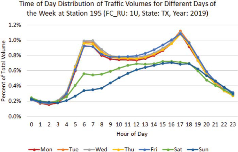
distinctive peaks in the morning and evening, as depicted in Figure 1, while on Saturdays and Sundays, the hourly distributions may have a single peak in the middle of the day. Rural roads often exhibit a single peak on all seven days of the week since traffic volumes usually increase during the day and decline in the evening.
Day-of-week patterns are prevalent across all vehicle types. Passenger car volumes tend to remain constant on weekdays and then decrease on weekends. Recreational travel routes may witness steady volumes on weekdays and surge on weekends. Trucks tend to exhibit single-mode patterns. The truck pattern peaks in the early morning since many trucks are employed for early
deliveries to assist businesses in preparing for the upcoming workday. Following this peak, truck activity gradually diminishes until early afternoon, after which it undergoes a rapid decline. Long-haul truck volumes often remain constant seven days a week, whereas short-haul trucks show weekday constancy with a more pronounced decline on weekends compared to passenger cars.
Monthly variations in traffic volumes are shaped by local socioeconomic activities and land uses. For instance, school-related traffic decreases during summer and winter breaks. Roads near beaches experience lower volumes in winter, whereas roads near ski resorts carry higher winter volumes. Monthly fluctuations in truck traffic are notable, especially in areas with agricultural or distribution hubs.
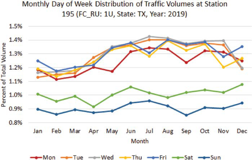
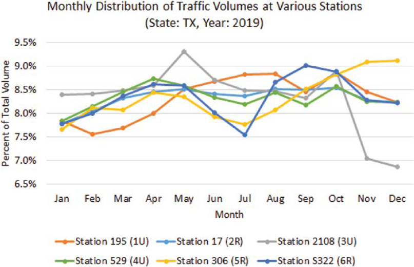
Figure 2 shows an example of monthly patterns by day of week at Station 195 in Texas. Though weekday traffic volumes tend to be higher and more similar than those on weekends, there are certain months during which traffic increases or decreases due to various local activities and planned or unplanned events. Figure 3 shows differences in monthly patterns of six sites located on roadways with different functional classes in Texas. Traffic monitoring programs need to review and consider these spatiotemporal differences from one site to another to identify sites with similar patterns, create homogeneous groups of sites, and then calculate group adjustment factors. The accuracy of AADT estimates derived from factored counts depends on whether the group adjustment factor(s) applied to the counts are representative of the actual temporal traffic patterns at each count location.
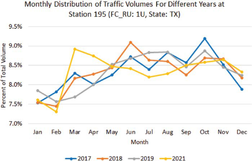
In addition to temporal variations, year-to-year changes may be evident in traffic patterns (Figure 4). These yearly fluctuations may be more pronounced when new developments that cause rapid growth are taking place or during economic downturns that lead to traffic volume decreases. Areas reliant on a particular economic sector witness dramatic volume changes based on sector growth or decline. For instance, during periods of high oil prices, rural roads with energy development activity may experience increased truck traffic until prices decrease.
Spatial variations occur at different geographical scales, from state-level disparities to differences between roadways and even locations along the same road or from one direction at a specific location to another. Similar variations exist for motorcycles, cars, and trucks. Roads of the same functional class, even in close proximity, can differ in traffic volumes due to geographical, socioeconomic, demographic, and land use distinctions. Geographic stratification is crucial for understanding roads with similar traffic characteristics, especially in states with diverse travel behavior. Even in urban areas, cities with heavy recreational movement exhibit different patterns than those without such travel. Directional variations may also be observed on certain roads, where traffic predominantly travels in one direction during the morning and the opposite direction in the afternoon. This directional pattern is common in suburban areas, with vehicles heading toward the city center in the morning and away from it in the afternoon.
AADT Estimation Errors
AADT values are subject to different sources of error depending on whether they are computed from CCS data or derived from factored counts.
AADT Errors from CCS Data
In general, AADTs calculated from CCS data are considered to be the most accurate values representing actual annual average traffic conditions when there is no missing data throughout the year, and the counting error associated with each set of permanent equipment is small. However, as explained below, these conditions are not always met throughout the year.
Errors Due to Missing Data
CCSs may experience equipment “downtime” one or multiple times per year. The data gaps created as a result of non-operational equipment can affect AADT accuracy. The larger the duration and the higher the frequency of missing data, the higher the impact on AADT accuracy. Krile et al. (2015) examined the impact of missing data on the accuracy of AADT calculated using the simple average approach (Equation 3), the AASHTO method, a modified version of the AASHTO method, and the equation recommended by TMG (Equation 5). The study concluded that the TMG equation is more robust in handling missing data than the other approaches and highlighted that even when data are not available for all 24 hours within a day, including data for some hours is important from an AADT accuracy perspective (Krile et al. 2015).
The traffic monitoring industry lacks a clear consensus regarding the acceptability of estimating missing or incomplete CCS data (AASHTO 2009). The TMG does not recommend any data imputation method. It follows the 2001 Data Quality Act guidelines and recommends that traffic monitoring programs should consider seven data quality principles (FHWA 2022).
The 2009 Guidelines for Traffic Data Programs provides some information related to dealing with missing data in Section 4.8 but does not explicitly recommend any data imputation method for traffic monitoring data (AASHTO 2009). There are numerous data imputation methods in the literature. Selecting one or more imputation procedures should account for the required precision of the results and the analysts’ ability to understand and implement the procedures.
When imputation procedures are used, analysts should prepare metadata by documenting and labeling the imputation processes used and the completeness of the data over time and space. For example, the temporal completeness of data can be expressed as a ratio of the number of records available to the total number of records expected. The spatial completeness of data refers to data being collected across all lanes in both directions of travel, if applicable. The computation of summary statistics should be avoided if long periods of data are missing at a CCS. Agencies that impute missing data should establish minimum (temporal and spatial) data completeness thresholds below which traffic statistics should not be summarized nor reported. The establishment of such thresholds should be based on research and empirical data. For more information regarding the imputation of CCS data, see Section 4.8 of the Guidelines for Traffic Data Programs (AASHTO 2009).
Errors Due to Various Factors Affecting Equipment Performance
Even when CCSs collect data continuously, their performance may be affected by a series of factors such as quality of installation, sensor calibration, environmental conditions, regular and appropriate maintenance, potential electromagnetic interference from nearby devices or infrastructure, the type of traffic being monitored, changes in traffic flow, sensor obstruction, and more. Depending on the type of equipment, some of these factors may have a larger impact on the accuracy of the data collected by each CCS. For example, inductive loops are insensitive to adverse weather conditions, but their accuracy may decrease when detecting a diverse range of vehicle classes, and wire loops are subject to high stresses of traffic. Piezoelectric counters tend to generate highly accurate classification data, but they are sensitive to temperature variations and may not perform well in slow or stopped traffic (FHWA 2006). The Traffic Detector Handbook (FHWA 2006) and the TMG (FHWA 2022) provide more information regarding the various types of traffic equipment along with their strengths and weaknesses.
Systematic and Random Counting Errors
Even when CCSs operate under ideal controlled conditions, and none of the aforementioned factors affect equipment performance, each type of equipment may exhibit systematic or random counting errors and have a certain level of accuracy and precision. In the case of CCSs, counting
errors tend to be small to negligible, making CCS data a common choice for benchmarking purposes in many research studies. The American Society for Testing and Materials (ASTM) has developed several standard terms and methods for installing, using, testing, and evaluating various traffic monitoring devices and data. The most relevant standards are:
- E177-20 Standard Practice for Use of the Terms Precision and Bias in ASTM Test Methods.
- E1318-09 Standard Specification for Highway Weigh-In-Motion (WIM) Systems with User Requirements and Test Methods.
- E1957-04 Standard Practice for Installing and Using Pneumatic Tubes with Roadway Traffic Counters and Classifiers.
- E2259-03a Standard Guide for Archiving and Retrieving Intelligent Transportation Systems-Generated Data.
- E2300-09 Standard Specification for Highway Traffic Monitoring Devices.
- E2467-05 Standard Practice for Developing Axle Count Adjustment Factors.
- E2532-09 Standard Test Methods for Evaluating Performance of Highway Traffic Monitoring Devices.
- E2759-10 Standard Practice for Highway Traffic Monitoring Truth-in-Data. (ASTM 2024)
Despite the limitations of each type of permanent equipment, CCSs are generally considered to produce more reliable and accurate data and traffic statistics, particularly AADT, than PTRs.
Some of the equipment and data issues described above can be mitigated, and the quality of the data can be improved by implementing appropriate data quality control and quality assurance protocols, conducting proactive and regular equipment maintenance, providing relevant staff training, and ensuring that these activities are performed as planned by well-trained personnel. Chapter 4 (Quality Assurance for Traffic Data) of the Guidelines for Traffic Data Programs (AASHTO 2009) provides comprehensive information related to traffic data quality such as basic definitions, attributes, metrics, considerations, criteria for identifying invalid data, and techniques for dealing with missing data.
The 2022 TMG also presents pertinent information, including a compendium of data quality control criteria and checks. Agencies should perform a comprehensive evaluation of traffic monitoring programs every five years (FHWA 2022). The purpose of these evaluations is to ensure compliance with relevant regulations, account for potential roadway changes, and address equipment and user needs. The activities described above should cover permanent and portable traffic counting equipment and data.
AADT Estimation Errors from Count Data
Similar to CCSs, PTRs can have data gaps and systematic and random counting errors. They can be affected not only by the factors mentioned above but also by other factors related to the temporary installation of PTRs (e.g., limited mounting options, durability, data transmission, data storage capacity, wireless connectivity, data security, etc.). Unlike the AADTs computed from CCS data, the AADTs estimated from short-term counts are subject to more sources of error generated from each step of the AADT estimation process, particularly the assignment step. These errors are described below.
Errors Stemming from the Computation of Individual Adjustment Factors for Each CCS
The first step in the AADT estimation process involves calculating individual adjustment factors for each CCS. The errors in this step are primarily caused by potential missing CCS data.
This not only impacts the accuracy of the computed AADT, which is the numerator in the adjustment factor calculation equation, but also that of the average volumes (e.g., MADT) used in the denominator of the same equation.
Errors Stemming from the Creation of Adjustment Factor Groups
The grouping step aims to create groups of CCSs or roads that exhibit similar traffic patterns (e.g., monthly or monthly day-of-week patterns) with low within-group variability, and are well-defined based on one or more characteristics so that any count or roadway segment can be easily assigned to a group. In practice, it is difficult to achieve both objectives. Statistical methods, such as cluster analysis, are effective in creating internally homogeneous groups by taking into account the variability in CCSs’ traffic patterns, but the produced clusters may not have any common characteristic to ease the assignment step. As a result, the group adjustment factors created for each cluster may be reliable and representative of all traffic patterns contained within a group but may not accurately capture the patterns of other locations for which CCS data do not exist. In contrast, traditional methods, such as functional classification, produce well-defined groups, which, nonetheless, may be internally heterogeneous. Consequently, the group adjustment factors may not be as reliable and effective in capturing all patterns within a group.
Errors Stemming from the Assignment Step
The assignment step involves assigning a count to a group of CCSs. The assignment process is the most critical part of the traditional AADT estimation method because the accuracy of the AADT estimates depends to a large degree on whether the adjustment factors applied to each count adequately capture the traffic patterns at the count location (Gulati 1995). Potential incorrect assignment of counts to adjustment factor groups may triple the AADT prediction error (Davis 1996). Research has shown that the AADT accuracy can be affected more by the assignment step than by the duration of counts (Sharma et al. 1996).
Errors Stemming from Misalignment of Factors with SDC Duration
Traffic patterns can vary within each month, such as by week and day of the month. However, the time intervals the temporal adjustment factors represent may not align with the duration of SDCs. For example, a monthly factor cannot capture the weekly variability within a month. When this factor is applied to a week-long count, it introduces a margin of error in the factoring process. Similarly, if a count spans across two consecutive months, similar errors will be generated.
Performance Metrics
The temporal adjustment factor groups created by any method during the grouping step have two key characteristics that can be quantified: the within-group variability and the precision of group adjustment factors. Furthermore, the AADT estimates produced by each method (after annualizing artificial SDCs extracted from CCSs) during the assignment step have a certain level of accuracy and precision that can be estimated as well. These four metrics can be used to compare the performance of two or more grouping/assignment methods. More information about each metric is provided below.
Within-Group Variability
Some methods, such as cluster analysis, tend to produce more homogeneous groups of CCSs in terms of temporal traffic patterns than others. The more similar the traffic patterns of the CCSs
within a group, the lower the within-group variability, indicating greater internal homogeneity within the group. To quantify the overall within-group variability of all factor groups created by a specific method, a weighted average coefficient of variation (WACV) can be computed following three steps.
- Step 1. The first step is to use Equation 2 to calculate the CV of each group adjustment factor from the corresponding individual adjustment factors of the CCSs within the group. For example, the CV of a group’s monthly day-of-week factor can be calculated as follows:
(10) Where:
CVm,j,k = coefficient of variation of group adjustment factor for month m and day-of-week j in factor group k.
sm,j,k = sample standard deviation of the CCSs’ individual adjustment factors for month m and day-of-week j in group (or cluster in the case of cluster analysis) k.
= average monthly day-of-week adjustment factor of group k for month m and day-of-week j.
- The first step yields 84 monthly day-of-week CVs for each group k created using a specific grouping method.
- Step 2. In the second step, an average coefficient of variation (ACV) can be calculated for each group as a simple average of the 84 CVs calculated in the first step:
(11) - Step 3. In the third step, a WACV can be calculated for all factor groups created by each method by accounting for the number of CCSs within each group.
(12) Where:
WACV = weighted average coefficient of variation of all groups developed using a specific grouping method. The lower the WACV, the more homogeneous the groups of a method.
nk = total number of CCSs within group k.
ng = total number of groups or clusters developed using a specific method.
Equations 10-12 can be simplified and applied if 12 monthly factors are used instead of 84 monthly day-of-week factors. A simple numerical example is provided below to illustrate these calculations. Assume that an analyst developed a Rural and an Urban group that contain 10 and 8 CCSs, respectively. Table 1 and Table 2 show the 12 monthly factors, the 12 CVs, and the ACVs of the two groups, respectively.
The CV for January in the Rural group is calculated as the standard deviation of the 12 monthly factors (1.040, 1.038, 1.154, 1.186, 1.020, 1.267, 1.081, 1.200, 1.257, 1.294) divided by the average value of these factors. The same calculation was performed for all CVs in both groups.
The ACV (5.81%) in the Rural group is calculated as a simple average of the 12 CV values: ACV = (8.95 + 7.78 + 4.50 + 3.62 + 3.59 + 7.18 + 8.07 + 5.16 + 7.16 + 2.85 + 4.14 + 6.76)/12
Table 1. Example of calculating CVs and ACV of a rural group containing 10 CCSs.
| CCS # | Monthly Adjustment Factors of Rural Factor Group | |||||||||||
|---|---|---|---|---|---|---|---|---|---|---|---|---|
| Jan | Feb | Mar | Apr | May | Jun | Jul | Aug | Sep | Oct | Nov | Dec | |
| 1 | 1.040 | 0.986 | 0.958 | 0.928 | 1.023 | 1.027 | 1.007 | 1.039 | 1.030 | 1.006 | 0.984 | 0.982 |
| 2 | 1.038 | 1.022 | 0.922 | 1.015 | 1.000 | 0.985 | 0.942 | 1.062 | 1.124 | 1.024 | 0.997 | 0.912 |
| 3 | 1.154 | 0.987 | 1.042 | 0.996 | 0.953 | 0.923 | 0.922 | 0.980 | 0.953 | 0.995 | 1.068 | 1.074 |
| 4 | 1.186 | 1.050 | 1.014 | 0.979 | 0.930 | 0.992 | 0.959 | 0.993 | 0.914 | 0.964 | 1.035 | 1.037 |
| 5 | 1.020 | 0.950 | 0.943 | 0.929 | 0.969 | 1.094 | 1.087 | 1.008 | 0.979 | 0.989 | 1.007 | 1.053 |
| 6 | 1.267 | 1.138 | 1.039 | 1.016 | 0.957 | 0.917 | 0.889 | 0.961 | 0.913 | 0.935 | 1.035 | 1.056 |
| 7 | 1.081 | 0.998 | 1.015 | 1.013 | 1.025 | 1.030 | 1.032 | 0.973 | 0.910 | 0.954 | 0.992 | 0.995 |
| 8 | 1.200 | 1.059 | 1.018 | 0.952 | 0.938 | 0.941 | 0.925 | 0.955 | 0.927 | 0.995 | 1.079 | 1.086 |
| 9 | 1.257 | 1.166 | 1.007 | 1.008 | 0.939 | 0.909 | 0.850 | 0.903 | 0.930 | 0.950 | 1.108 | 1.147 |
| 10 | 1.294 | 1.183 | 1.055 | 0.955 | 0.972 | 0.864 | 0.856 | 0.910 | 0.919 | 0.972 | 1.077 | 1.134 |
| CV | 8.95% | 7.78% | 4.50% | 3.62% | 3.59% | 7.18% | 8.07% | 5.16% | 7.16% | 2.85% | 4.14% | 6.76% |
| ACV | 5.81% | |||||||||||
Table 2. Example of calculating CVs and ACV of an urban group containing 8 CCSs.
| CCS # | Urban Factor Group | |||||||||||
|---|---|---|---|---|---|---|---|---|---|---|---|---|
| Jan | Feb | Mar | Apr | May | Jun | Jul | Aug | Sep | Oct | Nov | Dec | |
| 1 | 1.026 | 0.965 | 0.948 | 0.943 | 1.034 | 1.048 | 1.042 | 1.058 | 1.034 | 0.996 | 0.976 | 0.948 |
| 2 | 1.035 | 0.975 | 0.949 | 0.927 | 1.018 | 1.020 | 1.007 | 1.041 | 1.023 | 1.006 | 1.002 | 1.007 |
| 3 | 1.030 | 0.985 | 0.978 | 0.960 | 0.999 | 1.004 | 1.008 | 0.994 | 0.976 | 0.982 | 1.051 | 1.041 |
| 4 | 1.073 | 1.021 | 1.010 | 0.983 | 1.007 | 0.996 | 0.988 | 0.990 | 0.965 | 0.961 | 1.008 | 1.007 |
| 5 | 1.082 | 0.987 | 0.960 | 0.947 | 0.989 | 1.019 | 1.028 | 1.010 | 0.979 | 0.971 | 1.018 | 1.022 |
| 6 | 1.160 | 0.996 | 0.920 | 0.913 | 0.967 | 0.992 | 1.012 | 1.027 | 0.985 | 0.938 | 1.033 | 1.107 |
| 7 | 0.993 | 0.944 | 0.964 | 0.943 | 0.944 | 1.021 | 1.139 | 1.058 | 1.037 | 1.019 | 1.007 | 0.960 |
| 8 | 1.009 | 0.954 | 0.949 | 0.954 | 1.031 | 1.032 | 1.050 | 1.051 | 1.005 | 0.965 | 1.007 | 1.002 |
| CV | 5.05% | 2.50% | 2.72% | 2.22% | 3.14% | 1.83% | 4.52% | 2.71% | 2.81% | 2.71% | 2.18% | 4.88% |
| ACV | 3.11% | |||||||||||
After calculating the ACV of the Urban group (3.11%), the WACV is calculated using Equation 10 as follows:
The WACV (4.61%) captures the overall within-group variability of both groups developed based on the rural/urban area type.
Group Adjustment Factor Precision
The precision of a specific group adjustment factor reflects the consistency of the individual CCS adjustment factors used to calculate it. The precision accounts not only for the CV of each group adjustment factor but also for the sample size (i.e., number of CCSs) of a group. Similar to the WACV calculations, to quantify the overall group adjustment factor precision across all
groups created by a specific method, a weighted average precision (WAP) can be computed following three steps.
- Step 1. In the first step, the precision of a specific group adjustment factor can be calculated from Equation 1, which is also provided in the TMG. For example, the precision of a specific group monthly day-of-week adjustment factor can be calculated based on the assumption stated in the TMG that the existing CCSs “are equivalent to a simple random sample selection” (FHWA 2022):
(13) Where:
Pm,j,k = precision interval as a percentage of the group factor for month m and day-of-week j in group k.
t = value of Student’s T-distribution with 1 − α/2 level of confidence and n − 1 degrees of freedom.
α = significance level (0.05) for 95 percent confidence (α = 1 − 0.95).
- Step 2. After estimating the precision of each group factor, the average precision (AP) in each group can be calculated as follows:
(14) - Step 3. In the last step, a weighted average precision (WAP) can be calculated for all groups created by each method by accounting for the number of CCSs within each group.
(15) - Considering that some agencies do not conduct counts in all 12 months of the year, the WAP can be calculated based on the factors that are used to annualize SDCs.
AADT Accuracy
The AADT accuracy captures the closeness between AADT estimates derived from annualized sample counts extracted from CCSs and the actual AADTs calculated using CCS data. The closer the estimated AADTs are to the actual AADTs, the lower the AADT estimation errors or the higher the AADT accuracy. Commonly used accuracy metrics calculated for every pair of estimated AADT (AADTEst) and actual AADT (AADTAct) include:
| (16) |
| (17) |
| (18) |
| (19) |
After calculating one or more metrics for each pair of estimated AADT and actual AADT, various aggregate descriptive statistics (e.g., median, mean, standard deviation, percentiles, quantiles, etc.)
can be separately computed for each metric across all pairs or by slicing the results based on specific variables (e.g., mean absolute percent error [MAPE] broken down by functional class).
AADT Precision
The AADT precision reflects the closeness among AADT estimation errors. The closer the errors, the tighter the precision (i.e., low precision values), and vice versa. The AADT precision can be captured using several of the performance metrics and descriptive statistics discussed earlier in this chapter, such as the standard deviation of the PEs and the difference between two percentile values. For example, the difference between the 97.5th and the 2.5th percentiles of the PE captures the range or interval within which 95 percent of the entire population of AADT errors are expected to fall. The narrower the interval, the more precise the AADT estimates.


