Load Rating of Segmental Bridges (2024)
Chapter: 6 Execution of the Analytical Program
CHAPTER 6
Execution of the Analytical Program
6.1 Selection of the Set of Concrete Segmental Bridges
The objective of this task was to select a set of segmental bridges to be considered in this project. The selected set represents typical segmental bridges encountered in practice.
The team preselected eight DOTs from the following states to consult: Florida, Massachusetts, Texas, Colorado, California, Alabama, Michigan, and Minnesota. Based on the most recent (2023) data available from the NBI and InfoBridge, statistical analysis of segmental bridges was performed based on available bridge characteristics.
Selected bridge structures include those that are representative of location (chosen states), age, bridge maximum span length, total length, width, curvature, material type, rating method, and consequently, design live load model, traffic volume by ADTT, and condition.
These selection criteria were chosen based on the public domain data availability. Table 6-1 shows 50 preselected representative segmental bridge structures, where 41 bridges were selected from the chosen states, and nine bridges were selected based on the available bridge data from project partners. Of the nine bridges, one is in North Carolina and one is in Tennessee.
The broad spectrum of selected segmental bridges serves as a basis for developing new AASHTO rating procedures.
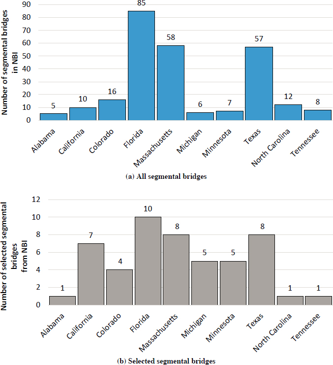
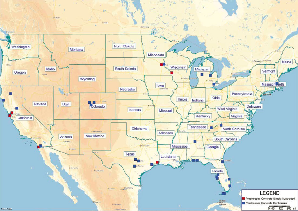
Statistical analysis of segmental bridges for preselected states was conducted. The filtering criteria for all segmental bridges in chosen states were compared to the selected sample data. Figure 6-1 presents the number of all segmental bridges for chosen states, and the number of selected segmental bridges for every state. The location of the selected segmental bridges is shown on the map (Figure 6-2).
The set of comparisons for all segmental bridges and selected segmental bridges is shown for bridge age, maximum span length, total length, number of approaching spans, number of lanes, ADTT per lane, superstructure condition rating, and operating rating method. Figure 6-3 presents the comparison of parameters along with the percentage of each group for the overall sample for selected and all segmental bridges.
6.2 Data Collection
In this step, the data required to conduct analyses of the selected bridges were collected. These data include information that reflects the current bridge condition (including inspection reports, field surveys, and relevant measurements), design and as-built plans, construction documents (contractor-proposed changes, shop drawings, casting and erection plans, material properties, casting records, construction loads, etc.), maintenance records (including repair and rehabilitation records), and rating reports (inventory and operating ratings).
Table 6-1. The 50 selected representative segmental bridges.
| State | Bridge ID | Year Built | Material | Max Span Length (ft) | Total Span Length (ft) | Number of Spans | Deck Width (ft) | Number of Lanes | Curvature (degree) | ADTT per Lane | Rating Method* | Superstructure Condition |
|---|---|---|---|---|---|---|---|---|---|---|---|---|
| Alabama | 6156780 | 2019 | P/C Cont. | 165 | 6,549 | 42 | 71 | 6 | 0 | 3,454 | No Rating | Good |
| California | 06 0210 | 2016 | P/C Cont. | 591 | 1,942 | 5 | 104 | 5 | 0 | 2,520 | Assigned LRFR | Good |
| 10 0299 | 2009 | P/C Cont. | 571 | 1,355 | 3 | 43 | 2 | 0 | 11 | Assigned LFR | Fair | |
| 24C0546 | 2009 | P/C Cont. | 430 | 970 | 3 | 82 | 4 | 0 | 2,244 | Assigned LFR | Fair | |
| 28 0153R | 2007 | P/C | 659 | 7,434 | 16 | 82 | 5 | 0 | 249 | Assigned LFR | Good | |
| 35 0331L | 2009 | P/C | 443 | 972 | 3 | 29 | 1 | 0 | 336 | Assigned LFR | Good | |
| 35 0331R | 2009 | P/C | 448 | 904 | 3 | 29 | 1 | 0 | 73 | Assigned LFR | Good | |
| 57 1186 | 2007 | P/C | 297 | 3,320 | 12 | 76 | 4 | 0 | 73 | Assigned LFR | Good | |
| Colorado | F-08-AV | 1989 | P/C Cont. | 210 | 1,320 | 7 | 35 | 2 | 0 | 1,020 | LFR | Good |
| F-11-AM | 1977 | P/C Cont. | 225 | 748 | 4 | 42 | 2 | Variant Skewness | 1,071 | LFR | Fair | |
| F-11-AN | 1977 | P/C Cont. | 225 | 748 | 4 | 42 | 2 | 0 | 1,071 | Field Evaluation | Fair | |
| H-09-U | 2005 | P/C Cont. | 270 | 620 | 3 | 73 | 2 | 0 | 391 | LRFR | Fair | |
| Florida | 100806 | 2006 | P/C Cont. | 142 | 17,001 | 122 | 60 | 3 | 0 | 1,585 | LFR | Good |
| 150189 | 1986 | P/C Cont. | 1200 | 21,877 | 11 | 95 | 4 | 0 | 474 | LRFR | Good | |
| 170176 | 2003 | P/C Cont. | 300 | 3,097 | 11 | 106 | 4 | Variant Skewness | 723 | LFR | Good | |
| 570091 | 1993 | P/C Cont. | 225 | 19,265 | 141 | 43 | 2 | 0 | 268 | LRFR | Fair | |
| 580174 | 1999 | P/C Cont. | 225 | 18,425 | 131 | 43 | 2 | 0 | 595 | LRFR | Fair | |
| 720640 | 2005 | P/C Cont. | 248 | 2,570 | 13 | 43 | 1 | Variant Skewness | 875 | LRFR | Good | |
| 860631 | 2002 | P/C Cont. | 190 | 784 | 5 | 97 | 6 | 0 | 148 | LFR | Fair | |
| 890151 | 1997 | P/C Cont. | 260 | 4,487 | 21 | 61 | 3 | 0 | 408 | LFR | Good | |
| 900101 | 1982 | P/C Cont. | 135 | 35,868 | 266 | 39 | 2 | 0 | 474 | LRFR | Fair | |
| 900117 | 1981 | P/C Cont. | 118 | 4,557 | 39 | 39 | 2 | 0 | 2,170 | LRFR | Fair | |
| Massachusetts | B16600900 | 2003 | P/C Cont. | 143 | 547 | 4 | 54 | 3 | 0 | 1,118 | LFR | Fair |
| B166018YX | 2002 | P/C Cont. | 143 | 715 | 5 | 67 | 5 | 0 | 1,317 | LFR | Fair | |
| B166038DF | 2005 | P/C Cont. | 147 | 1,029 | 7 | 36 | 2 | 0 | 255 | LFR | Good | |
| B166118Y3 | 2001 | P/C Cont. | 163 | 697 | 5 | 29 | 1 | Variant Skewness | 1,874 | LFR | Fair | |
| B166569AJ | 2000 | P/C Cont. | 150 | 300 | 2 | 90 | 6 | 0 | 411 | LFR | Fair | |
| B166618QY | 2002 | P/C Cont. | 154 | 667 | 5 | 51 | 3 | 9 | 864 | LFR | Fair | |
| B166629Q3 | 2006 | P/C Cont. | 142 | 283 | 2 | 43 | 2 | 0 | 200 | AS | Fair | |
| B166818QV | 2002 | P/C | 105 | 111 | 1 | 60 | 4 | 4 | 1,072 | LFR | Fair |
| Michigan | 6717 | 1983 | P/C Cont. | 270 | 580 | 3 | 46 | 2 | 0 | 657 | LRFR | Good |
| 9168 | 1980 | P/C Cont. | 392 | 8,061 | 25 | 75 | 4 | 0 | 657 | LRFR | Fair | |
| 9169 | 1984 | P/C Cont. | 392 | 8,085 | 26 | 75 | 4 | 0 | 689 | LRFR | Fair | |
| 9170 | 1984 | P/C Cont. | 243 | 648 | 4 | 29 | 1 | 0 | 106 | LRFR | Fair | |
| 11148 | 1984 | P/C Cont. | 181 | 1,567 | 5 | 36 | 2 | 0 | 492 | LFR | Good | |
| Minnesota | 27409 | 2008 | P/C | 505 | 1,221 | 4 | 92 | 5 | 0 | 1,008 | LRFR | Good |
| 27410 | 2008 | P/C | 498 | 1,228 | 4 | 90 | 5 | 0 | 1,008 | LRFR | Good | |
| 82045 | 2017 | P/C Cont. | 600 | 5,079 | 6 | 98 | 4 | 0 | 359 | LRFR | Fair | |
| 85801 | 2016 | P/C | 508 | 2,593 | 4 | 45 | 2 | 0 | 718 | LRFR | Good | |
| 85802 | 2015 | P/C | 180 | 2,593 | 4 | 37 | 2 | 0 | - | LRFR | Good | |
| North Carolina | 5140182P | 1983 | P/C Cont. | 508 | 1,249 | 8 | 45 | 2 | 0 | 718 | LRFR | Good |
| Tennessee | 5460214P | 2013 | P/C Cont. | 180 | 790 | 5 | 38 | 2 | 0 | 340 | AS | Good |
| Texas | 1.2102E+14 | 1980 | P/C Cont. | 750 | 10,538 | 1 | 60 | 4 | 0 | 1,144 | Assigned LFR | Fair |
| 1.4027E+14 | 2012 | P/C Cont. | 410 | 958 | 1 | 47 | 2 | 0 | 296 | Assigned LRFR | Good | |
| 1.4227E+14 | 1998 | P/C | 134 | 4,108 | 34 | 58 | 2 | 0 | 658 | Assigned LFR | Fair | |
| 1.4227E+14 | 1998 | P/C Cont. | 178 | 1,943 | 15 | 28 | 1 | 0 | 1,902 | Assigned LFR | Fair | |
| 1.5015E+14 | 1991 | P/C Cont. | 101 | 281 | 3 | 26 | 1 | 0 | 304 | No Rating | Good | |
| 1.5015E+14 | 1993 | P/C Cont. | 106 | 1,345 | 14 | 74 | 5 | Variant Skewness | 512 | No Rating | Fair | |
| 1.6178E+14 | 1973 | P/C Cont. | 200 | 3,280 | 1 | 56 | 4 | 0 | 676 | Field Evaluation | Fair | |
| 2.0181E+14 | 2015 | P/C | 320 | 3,896 | 3 | 70 | 3 | 0 | 1,469 | No Rating | Good |
*LFR: Load Factor Rating; AS: Allowable Stress; LRFR: Load and Resistance Factor Rating; Assigned LFR: Assigned Load Factor Rating for HS 20; Assigned LRFR: Assigned Load and Resistance Factor Rating for HL-93.
A DOT survey was conducted to gather essential data for performing the reliability-based analysis of segmental bridges. An important part of data collection is the identification of construction methods (balanced cantilever, span-by-span, etc.) and information about erection procedures (such as cantilever alignment and segment age when erected). Table 6-2 presents the data request, which was sent to DOTs for the 50 selected segmental bridges.
The team also collected information on as-inspected deterioration data and the effect on load rating from examples available from the team’s industrial partners. To incorporate the bridge deterioration into the load rating analysis, the team performed the following steps:
- Collect bridge deterioration information and data; inspection reports going back multiple cycles were requested from various participating states.
- Categorize the major/dominant deterioration modes on segmental concrete bridges (e.g., section loss of post-tensioned reinforcement) based on field data and expert opinions.
- Evaluate how the deterioration modes impact the bridge load rating in terms of specific structural components and limit states.
- Summarize the findings and possible ways of incorporating deterioration into a detailed load rating analysis.
In addition to the bridge condition ratings from inspections, two types of condition ratings data are available, including NBI component ratings and AASHTO element ratings. The team collected data and investigated whether and how to use these data in the load rating analysis.
Four state DOTs provided the data on the segmental bridges as shown in Table 6-3.
6.3 Selection of Limit States
Based on a review of the rating information and preliminary analysis of the structures identified in Section 6.1, as well as input from segmental bridge experts, including those on the research team and ASBI and state transportation agencies, appropriate limit states were identified for service and strength levels. The following five limiting criteria were considered:
- Service limit state
- Flexural tensile stress
- Flexural compressive stress
- Principal tensile stress (combined flexural, shear, and torsional effects)
- Strength limit state
- Flexural strength
- Shear strength (from combined direct shear and torsion)

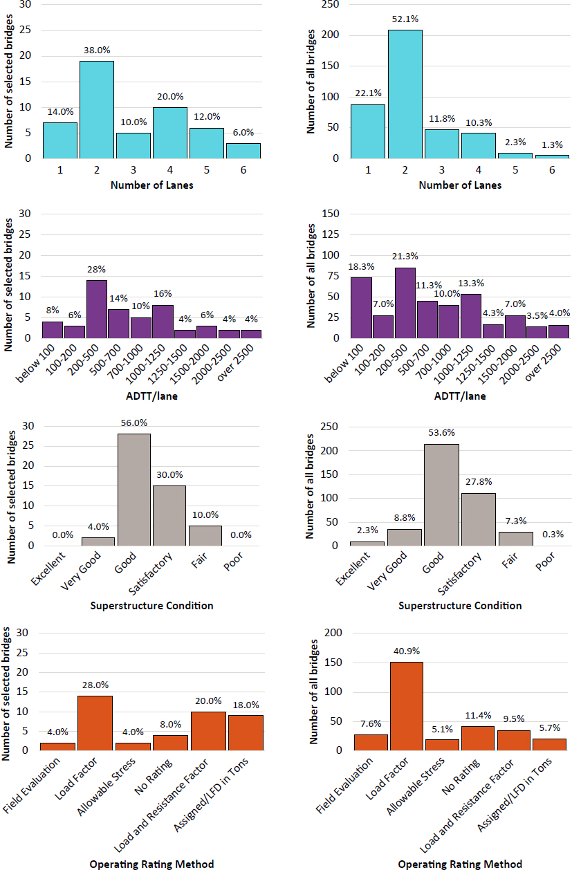
Table 6-2. DOT data collection for segmental bridges.
| Item | Description |
|---|---|
| Bridge Inspection Report | Most recent and historical bridge inspection reports for selected bridges (Table 6-1). |
| Field Surveys | Performed detailed bridge surveys. |
| Field Measurements | Bridge field testing for bridge evaluation or other reasons. |
| Design Plans | Detailed drawings including cross-section properties, with an indication of variable/constant depth, internal and external tendons, etc. |
| As-Built Plans | Post-construction drawings. |
| Construction Shop Drawings | Construction drawings, including balanced cantilever, span-by-span, etc. |
| Casting and Erection Plans | Erection scheme and plan procedures, such as cantilever alignment and segment age when erected. |
| Material Properties | Material properties and testing data. |
| Casting Records | - |
| Construction Loads | - |
| Maintenance Records (including repair and rehabilitation) | Any maintenance activities and their descriptions. |
| Segmental Bridge Deterioration | Major deterioration modes on segmental concrete bridges. |
| Rating Reports: Inventory and Operating Rating Calculations | Rating reports, including calculation of section capacities for all limit states, transverse, and longitudinal analysis results. |
| Rating Cards | Summary of the calculated ratings and safe live load-carrying capacities. |
| NBI Component Ratings | NBI component rating description. |
| AASHTO Element Ratings | AASHTO component rating description. |
| Rating issues | Describe any segmental bridge rating issues. |
| Long-term monitoring data | Long-term monitoring data if available. |
| Creep and Shrinkage Models | Creep and shrinkage models selected during design. |
Table 6-3. Segmental bridge data collected from state DOTs.
| State | No. of Bridges | Types of Data |
|---|---|---|
| California | 14 | Bridge inspection reports, design plans. |
| Colorado | 16 | Inspection sketches, photographs, design plans, load rating information. |
| Massachusetts | 57 | Bridge inspection reports, design plans load rating reports. |
| Michigan | 2 | Design plans, load rating reports. |
Consideration must be given to joint behavior. Thus, in the longitudinal direction, these limit states were at each joint. Similar checks were conducted in the transverse direction.
The service limit states are consistent with the previous service limit state calibration work conducted under NCHRP Project 12-83. The team identified the stress limits at service limit state for longitudinal and transverse analysis as shown in Table 6-4 [based on FDOT’s New Directions for Florida Post-Tensioned Bridges (Corven Engineering 2004)].
Table 6-4. Stress limits in concrete at the inventory and operating ratings for segmental bridges.
| At the Service Limit State After Losses | Stress Limit Inventory Rating | Stress Limit Operating Rating | Source of Criteria |
|---|---|---|---|
Compression (Longitudinal or Transverse)
| LRFD Table 5.9.2.3.2a-1 LRFD Article 5.6.4.7.2c | ||
Longitudinal Tensile Stress in Precompressed Tensile Zone (intended for segmental and similar construction)
| 0.3 ksi tension | ksi tension | LRFD Table 5.9.2.3.2b-1 and FDOT no distinction for environment |
| No tension | No tension | LRFD Table 5.9.2.3.2b-1 |
Longitudinal Tensile Stress through Joints in Precompressed Tensile Zone (intended for segmental and similar construction)
| 0.3 ksi tension | ksi tension | LRFD Table 5.9.2.3.2b-1 Seg. Guide Spec. 9.2.2.2 FDOT has no distinction for environment |
| No tension | No tension | Ditto and FDOT Seg. Rating Criteria |
| 0.1 ksi min comp. | No tension | Seg. Guide Spec. 9.2.2.2 FDOT Seg. Rating Criteria |
Transverse Tension, Bonded PT
| 0.3 ksi tension | ksi tension | Seg. Guide Spec. 9.2.2.3 LRFD Table 5.9.2.3.2b-1 FDOT has no distinction for environment FDOT Seg. Rating Criteria |
| At the Service Limit State After Losses | Stress Limit Inventory Rating | Stress Limit Operating Rating | Source of Criteria |
|---|---|---|---|
Tensile Stress in Other Areas
| Seg. Guide Spec. 9.2.2.4 | ||
| ksi tension | ksi tension | LRFD Table 5.9.2.3.2b-1 Seg. Guide Spec. 9.2.2.4 LRFD Table 5.9.2.3.2b-1 |
Principal Tensile Stress at Centroidal Axis in Webs (Service III)
| ksi tension | ksi tension | LRFD 5.9.2.3.3 FDOT LRFR Rating Criteria |
| * Principal tensile stress is calculated for longitudinal stress and maximum shear stress due to shear or combination of shear and torsion, whichever is greater. For segmental box, check centroidal axis. For composite beam, check at centroidal axis of beam only and at centroidal axis of composite section, and take the minimum value. Web width is measured perpendicular to the place of web. For segmental box, it is not necessary to consider coexistent web flexure.
Account should be taken of vertical compressive stress from vertical PT bars provided in the web, if any, but not including vertical component of longitudinal draped post-tensioning. The latter should be deducted from shear force due to applied loads. Check section at H/2 from edge of bearing or face of diaphragm, or at end of anchor block transition, whichever is more critical. For the design of a new bridge, a temporary principal tensile stress of kis may be allowed during construction, per AASHTO Seg. Guide Spec. Initial load ratings for new design should be based upon specified concrete strength. Load rating of an existing bridge should be based on actual concrete strength from construction or subsequent test data. | |||
6.4 Comparative Analysis That Includes Comparison with Field Data
6.4.1 Introduction
A comparative analysis was conducted to evaluate the influence of several factors on the load rating of concrete segmental bridges in the longitudinal direction. This comparative analysis was conducted to aid the engineer in understanding the impact that certain assumptions have on the load rating of concrete segmental bridges. The investigated factors and parameters included the following:
- Influence of the selection of creep and shrinkage models on load rating.
- Influence of temperature gradient compared to other load cases on load rating.
- Influence of compressive strength overstrength factors on load rating.
- Influence of the selection of time-dependent concrete strength development model on load rating.
- Influence of various load cases on principal tensile stress in the web and impact of assumed allowable tensile stress on load rating.
- Influence of condition factors on load rating.
- Influence of the use of transformed versus gross-section properties on load rating.
- Influence of time when the load rating is conducted on load rating factors.
- Influence of multiple trucks on load rating.
While a total of four load rating examples are presented for bridges constructed with (1) the span-by-span method, (2) balanced cantilever method, (3) incremental launching method, and (4) a cable-stayed bridge, the comparative analysis was conducted for the bridges constructed
Table 6-5. Outline of load rating analysis.
| Analysis Level | Analysis Direction | Load Combinations | Limit States |
|---|---|---|---|
| Inventory | Longitudinal | Service I/III | Flexure (compression and tension) |
| Principal Web Tension (flexure, shear, and torsion) | |||
| Strength I | Flexural Strength | ||
| Shear Strength (considering torsional effects) | |||
| Transverse | Service I | Top Slab Flexure | |
| Strength I | Top Slab Flexural Strength |
with the span-by-span and balanced cantilever method. The influence of (1) time when the load rating is conducted, (2) the use of transformed versus gross-section properties, and (3) multiple trucks on load rating was conducted only for the concrete segmental bridge constructed with the balanced cantilever method. The bridges used to prepare the load rating examples represent simplified versions of real bridges (Midas Civil 2023). All bridges feature internally bonded tendons. The load rating examples (Appendix C of the Guideline) provide detailed information about the load rating of the abovementioned four bridges. Section C.1 in the load rating examples presents detailed information about the assumptions made during the analysis. A summary of key points is repeated here for convenience. All bridges considered were load rated at the inventory level considering Service I/III and Strength I load combinations. The outline of the analysis as well as the considered limit states are presented in Table 6-5 and the load factors used for each load combination are presented in Table 6-6. The strength reduction factors were based on AASHTO LRFD (2020a). Condition factors and system factors were based on AASHTO MBE (2020b). Multiple presence factors (MPFs) were based on AASHTO LRFD (2020a). Flexural strength was based on AASHTO LRFD (2020a) provisions for prestressed concrete cross sections with internally bonded tendons. Although Corven Engineering (2004) recommends the use of actual material properties when calculating flexural strength, specified material properties were used because this information was not available for the bridges considered. Shear strength was based on AASHTO LRFD (2020a) alternative shear provisions for concrete segmental bridges. The combination of torsional and shear effects at service and at ultimate limit state was based on AASHTO LRFD (2020a). Allowable stresses in concrete segments for load rating were based on the recommendations provided by Corven Engineering (2004).
Table 6-6. Load factors and combinations for the design load rating at the inventory level for HL-93.
| Analysis | LRFD Permanent Load | LRFD Transient Loads | ||||||||
|---|---|---|---|---|---|---|---|---|---|---|
| γDC | γDW | γEL | γPS | γCR,SH | γFR | γTU | γTG | γLL | ||
| Long. | Strength I | 1.25 | 1.50 | 1.00 | 1.00 | 1.25 | 1.00 | 0.00 | 0.00 | 1.75 |
| Service I/III | 1.00 | 1.00 | 1.00 | 1.00 | 1.00 | 1.00 | 1.00 | 0.50 | 0.80 | |
| Trans. | Strength I | 1.25 | 1.50 | 1.00 | 1.00 | 1.25 | 1.00 | 0.00 | 0.00 | 1.75 |
| Service I | 1.00 | 1.00 | 1.00 | 1.00 | 1.00 | 1.00 | 1.00 | 0.50 | 0.80 | |
| γDC: load factor for structural components; γDW: load factor for permanent superimposed dead loads; γEL: load factor for locked-in construction stresses; γPS: load factor for prestressing effect; γFR: load factor for bearing friction or frame action; γCR,SH: load factor creep and shrinkage; γTU: load factor for uniform temperature load; γTG: load factor for thermal (temperature) gradient; and γLL: load factor for live load. | ||||||||||
The load rating factors (RFs) were calculated using Eqs. (6-1 through 6-4).
| (6-1) |
For the strength limit states:
| (6-2) |
| (6-3) |
For the service limit states:
| (6-4) |
where
| DC = | dead load of structural components and nonstructural attachments. |
| DW = | dead load of wearing surfaces and utilities. |
| PS = | secondary forces from post-tensioning for strength limit states; total prestress forces for service limit states. |
| EL = | miscellaneous locked-in force effects resulting from the construction process, including jacking apart of cantilevers in segmental construction. |
| FR = | friction load. |
| TU = | force effect due to uniform temperature. |
| CR = | force effects due to creep. |
| SH = | force effects due to shrinkage. |
| TG = | force effect due to temperature gradient. |
| LL = | vehicular live load. |
| IM = | vehicular dynamic load allowance. |
| γDC = | load factor for structural components. |
| γDW = | load factor for permanent superimposed dead loads. |
| γEL = | load factor for secondary post-tensioning effects and locked-in erection loads. |
| γFR = | load factor for bearing friction or frame action. |
| γCR,SH = | load factor for creep and shrinkage. |
| γTU = | load factor for uniform temperature. |
| γTG = | load factor for temperature gradient. |
| γLL = | load factor for live load. |
| C = | capacity. |
| ϕc = | condition factor. |
| ϕs = | system factor. |
| ϕ = | resistance factor per LRFD. |
| Rn = | nominal member resistance as inspected, measured, and calculated according to formulas in LRFD. |
Unless otherwise noted, the baseline or benchmark case used in the comparative analysis included the following options:
- CEB-FIP (1990) model was used for predicting creep and shrinkage behavior, and concrete compressive strength development with time.
- AASHTO LRFD (2020a) model was considered for the calculation of modulus of elasticity of concrete at 28 days.
- No overstrength factors were used (i.e., specified concrete compressive values were considered).
- Transformed-section properties were used.
- Load rating was conducted at 10,000 days after the completion of the bridge.
- The structure was assumed to be subject to a ± 70 °F uniform temperature change.
- The temperature gradient effects were based on AASHTO LRFD (2020a) solar radiation zone 3.
A comparative analysis was also conducted in the transverse direction and included a comparison of live load effects obtained using Homberg charts and a 2D frame model, a 3D shell FE model, and field data for the Seabreeze Bridge located in Daytona, Florida.
A general discussion of several of the considered factors is presented. The quantification of the influence of each factor is provided in the subsequent sections.
6.4.1.1 Creep and Shrinkage
Currently, AASHTO LRFD (2020a) Article 5.4.2.3.1 states that where mix-specific data are not available, estimates of shrinkage and creep may be made using the provisions of any of the following: (1) the creep and shrinkage models in AASHTO LRFD (2020a) Articles 5.4.4.3.2 and 5.4.4.3.3; (2) the fib Model Code for Concrete Structures (fib 2010); (3) the CEB/FIP Model Code for Concrete Structures (CEB-FIP 1990), or ACI 209. In addition, it is stated that for concrete segmental bridges, a more precise estimate shall be made, including the effect of all the following: (1) specific materials, (2) structural dimensions, (3) site conditions, (4) construction methods, and (5) concrete age at various stages of erection. It should be noted that ACI Committee 209 presents four models in the appendix of ACI 209.2R-08 namely: (1) ACI 209R-92 model, (2) Bažant-Baweja B3 model, (3) CEB MC90-99 model, and (4) GL2000 model [developed by Gardner and Lockman (2000)]. This leaves the engineer with a plethora of options when it comes to the selection of creep and shrinkage models for load rating concrete segmental bridges. The impact that the selection of creep and shrinkage models has on load rating is reflected in (1) the computation of prestress losses, and (2) the computation of secondary forces created due to the statical indeterminacy of the bridge as well as those created due to force redistribution due to creep effects. The impact that the selection of a particular creep and shrinkage model has on load rating was investigated for a bridge constructed with the span-by-span and another constructed with the balanced cantilever method. The following creep and shrinkage models were considered: (1) CEB-FIP 1990, (2) fib 2010, (3) CEB-FIP 1978, (4) AASHTO LRFD (2020a), and ACI 209R-92. The inclusion of CEB-FIP 1978 was done to evaluate the influence of creep and shrinkage models that were used extensively by the concrete segmental bridge community in the past on the load rating of concrete segmental bridges. When it comes to the evaluation of various creep and shrinkage models, it should be noted that there is no agreement as to which statistical indicator(s) should be used, which data sets should be used, or what input data should be considered [ACI Committee 209 (2008)].
6.4.1.2 Influence of Temperature Gradient on Load Rating
The influence of positive and negative temperature gradients on the load rating of concrete segmental bridges was investigated by considering the two bridges mentioned previously. Stresses created by temperature gradients were compared with those created by other load cases. Temperature gradients for various solar radiation zones were considered to illustrate the impact that the geographic position of the bridge or other research-based temperature gradients that differ from those presented in AASHTO LRFD (2020a) had on load rating.
6.4.1.3 Compressive Strength Overstrength Factors
Compressive strength overstrength factors are herein defined as the ratio of expected to specified concrete compressive strength. The use of expected rather than specified concrete compressive strength resulted in higher rating factors through two mechanisms: (1) an increase in the allowable stresses, which are typically expressed as a function of concrete compressive strength, and (2) the impact that the use of a stronger concrete has on the time-dependent structural analysis. Both these aspects were investigated. A total of four overstrength factors were considered: 1.0, 1.1, 1.2, and 1.3. The overstrength factors were applied to the specified concrete compressive strength at 28 days.
6.4.1.4 Models for Predicting Concrete Compressive Strength Development over Time
Since the compressive strength of concrete varies with time, the influence of the selected model for predicting this variation on load rating was investigated. The models considered for predicting the variation of concrete compressive strength with time were (1) ACI 209R-92 (ACI 1992), and (2) fib (2010). The variation of compressive strength with time affects the variation of modulus of elasticity with time, which is predicted using functions expressed in terms of the compressive strength. The time-dependent modulus of elasticity is, on the other hand, used to determine time-dependent transformed-section properties, and the effective modulus is used to account for creep effects.
6.4.1.5 Influence of Various Load Cases on Principal Tensile Stress in the Web and Impact of Assumed Allowable Tensile Stress
Since the load rating of concrete segmental bridges is controlled primarily by the service limit state, the impact that the selected allowable tensile stress has on load rating was investigated by considering various allowable tensile stress values for the principal tensile stress in the web. The considered allowable tensile stresses included (1) Zero tension, (2) ksi, (3) ksi, (4) ksi, and (5) ksi. In addition, the contribution of each load case to the principal tensile stress in the web was quantified. The guidance on selecting a value for the allowable principal tensile stress varies in terms of design and load rating. AASHTO LRFD (2020a) specifies a value of ksi and indicates that a factor of 0.8 should be used for live load (Service III). Corven Engineering (2004) recommends a value of ksi and a live load factor of 0.8 (Service III) for inventory rating.
6.4.1.6 Influence of Condition Factors on Load Rating
Currently, condition factors are used as a metric to characterize deterioration. In the current formulation, condition factors affect the strength limit states (flexural and shear strength). The report by Corven Engineering (2004) provides guidance for how to determine condition factors for concrete segmental bridges. The recommendations were developed by extending the concepts of “structural condition” given in LRFR to the particulars of concrete segmental bridges.
The selection of condition factors for each limit state should be conducted such that it reflects the current condition of the bridge and with consideration for how that condition affects the limit state of interest. For example, Corven Engineering (2004) reports that if corrosion damage to bonded tendons is localized to one region or to one or more particular cross sections and the rest of the structure is otherwise satisfactory, then the low value (0.85) may be applied to those areas and an appropriately higher value to others. However, caution is advised since damage to an internal tendon at one section may mean that it may be partially effective at other sections.
The influence of condition factors on load rating was quantified by assuming different values for the condition factor and by load rating the bridge based on these assumptions.
6.4.1.7 Transformed versus Gross-Section Properties
The sequential nature of construction in concrete segmental bridges includes forces that are applied to the net concrete cross section, such as when post-tensioning is applied, and forces that are applied to the transformed concrete cross section, such as those created by loads applied after the grouting process in the ducts is completed for bridges that feature internally bonded tendons. The impact of the selection of gross- versus transformed-section properties was investigated by conducting load rating computations for each case. The use of transformed versus gross-section properties is typically left to the discretion of the engineer. Maguire et al. (2015) used uncracked, transformed-section properties, including tendons, mild reinforcement, barrier rails, and full flange width for their beamline elements in their beamline longitudinal model. In this investigation, the presence of barrier rails was ignored in the definition of the cross section and the calculation of the section properties. Transformed-section properties included the presence of tendons, whereas gross-section properties were based solely on the concrete segmental cross section.
6.4.1.8 When the Load Rating Was Conducted
To quantify the impact that the time the bridge was rated has on the outcome of the rating, three cases were considered in terms of when the bridge was load rated. The baseline case used in all analyses was 10,000 days after the completion of construction and the opening of the bridge to traffic. The concrete segmental bridge constructed with the balanced cantilever method was load rated two more times at 5,000 days and 15,000 days after the completion of construction and the opening of the bridge to traffic.
6.4.1.9 Influence of Multiple Trucks
The evaluation of the presence of multiple trucks is conducted in two ways. First, the influence of lane configuration on load rating is determined for the concrete segmental bridge constructed with the balanced cantilever method. This is addressed in Section 6.4.5.10. The considered lane configurations include one based on design lanes (three lanes in this case) and another based on striped lanes (two in this case). For each case, the bridge is rated in the longitudinal and transverse directions. While the number of lanes was based on either design or striped lanes, the position of live load in the transverse direction was determined such that it created the worst-case effects based on the limitations provided in AASHTO MBE (2020). Second, the impact of multiple trucks within a given lane configuration was evaluated by considering the results obtained from the three load rating examples that addressed bridges constructed with the span-by-span, balanced cantilever, and incremental launching method. This situation is addressed in Section 6.4.6.
6.4.1.10 Influence of Analysis Technique on Live Load Effects in the Transverse Direction
Computed live load induced strains in the top slab in the transverse direction based on a 2D frame model and influence surfaces as well as on 3D finite element analysis were compared with those measured during a live load test for the Seabreeze Bridge, in Daytona, Florida. The goal of this comparison is to determine the level of conservatism used in the traditional frame analysis and to make recommendations for load rating.
6.4.1.11 Influence of Erection Time
The influence of erection time on load rating factors is investigated for a three-span concrete segmental bridge constructed with the span-by-span method. A comparison of rating factors is conducted assuming two erection scenarios. In the first scenario, it is assumed that two spans are erected each week. In the second scenario, it is assumed that one span is erected each week.
A study of the influence of erection on the balanced cantilever bridge is not included in this report. Such a study would include considering two different erection schedules while maintaining the same production date of the precast segments. In this scenario, the slower erection schedule would lead to the erection of older segments, which would then experience lower time-dependent stress changes, albeit with them having slightly higher stiffness as a function of increased age. In general, for the three-span bridge of Example 2, at some bridge age where time-dependent behavior has ceased, the load ratings of the more slowly erected bridge would be higher at midspan (positive bending) and lower at the piers (negative bending) than those of the bridge erected faster.
6.4.1.12 Influence of the Resal Effect
The influence of the Resal effect on load rating was investigated for the bridge constructed with the balanced cantilever method. The investigated limit state was vertical shear at the ultimate load level. Rating factors for this limit state were computed once by ignoring the Resal effect, and another time by considering it. The percentage change in rating factors was quantified. Taking account of the Resal effect may improve ratings related to principal tension in the webs.
6.4.2 Numerical Modeling Protocol and Load Rating Analysis
The bridges constructed with the span-by-span, balanced cantilever, and incremental launching methods and discussed in the load rating examples were load rated in the longitudinal and transverse directions.
Longitudinal Direction
In the longitudinal direction, the time-dependent structural analysis was conducted in Midas Civil 2023. The analysis results were exported to an Excel file, which in turn served as an input file for load rating calculations in Mathcad 15. For every segment, at the i-joint (the beginning of the segment) and j-joint (the end of the segment), load demand in terms of axial force, bending moment, shear, and torsion were exported to the Excel file. In addition, for every segment at the i-joint and j-joint, sectional capacities in terms of flexural strength and shear strength, computed in Midas Civil 2023, were exported to the Excel file. These flexural and shear capacities were verified with independent manual calculations based on AASHTO LRFD (2020a) as explained in the load rating examples (Appendix C of the Guideline). Similarly, for every segment at the i-joint and j-joint, the section properties in terms of area, moment of inertia, centroidal axis, first moment of area, area enclosed by shear flow path (including any areas of holes therein), and length of median of web measured on slope from mid-depth of top slab to mid-depth of bottom slab were exported to the Excel file. Once this information was exported to Excel, the load rating factors were calculated for each joint, each limit state, and each load combination. These load rating factors were then plotted as a function of segment number to illustrate their variation and to identify controlling segments and locations. An algorithm was created in Mathcad to compute the load rating factors for each of the cases mentioned at each joint.
Temperature gradient was based on solar radiation zone 3. Stresses created due to temperature gradient (self-equilibrating and secondary axial force and bending moment stresses) were obtained from Midas Civil 2023, although independent manual calculations based on free, restrained, and self-equilibrating stresses were conducted to validate the accuracy of the results. This situation is discussed further in the validation section. The uniform temperature change load case (TU) did not create any stress effects in the bridge constructed with the span-by-span method because the superstructure was free to axially contract or expand. In the bridge constructed by the balanced cantilever method, stresses created due to TU were considered because the superstructure and pier were rigidly connected.
The analytical model used to conduct the time-dependent structural analysis in the longitudinal direction was a 3D model featuring beam finite elements for the concrete segments. Timoshenko beam elements were used for the concrete segments. Each beam element featured a total of six degrees of freedom per node, three translational and three rotational. The use of Timoshenko beam elements rather than Euler-Bernoulli beam elements allowed the consideration of shear deformations. Prestressing effects were simulated using the equivalent load concept based on specified tendon coordinates. The stiffness of the tendons was reflected in the computation of transformed-section properties. The tensile stresses in the tendons, which were used to calculate the equivalent loads, were based on the prestress losses at every construction stage caused by various factors such as creep and shrinkage of concrete, relaxation of prestressing strands, friction losses, anchorage seating losses, and elastic losses or gains. While prismatic concrete segments were used for the bridge constructed by span-by-span method, linearly varying segments were considered for the bridge constructed by balanced cantilever method to capture the variable stiffness of the segments. The variation of depth within a segment was considered to be linear. The pier elements for the bridge constructed with the balanced cantilever method were prismatic elements. The analytical model is capable of capturing (1) staged construction; (2) time-dependent effects; and (3) prestress losses due to creep, shrinkage, relaxation, friction, anchorage set, and elastic loss or gain. Both short-term and long-term prestress losses were considered. Short-term losses included (1) elastic shortening losses (or elastic elongations gains), which were captured through strain compatibility by the analytical model as the structure deforms; (2) anchorage set losses, which were calculated based on specified anchorage set, friction, and wobble factors; and (3) friction losses, calculated based on selected code formula, tendon geometry, and friction and wobble factors. Long-term losses included (1) creep and shrinkage, which were calculated together based on strain compatibility for each construction stage, and (2) relaxation losses which were calculated based on Eq. (6-5) (Magura et al. 1964). The calculation of the relaxation loss was based on an assumed variation of the initial prestressing force at each time step. Eq. (6-5) is similar to the AASHTO LRFD (2020a) Eq. 5.9.3.4.2c-1.
| (6-5) |
A node located at mid-width of the segment and at the top of the segment was used as the reference node to define the superstructure for the bridge constructed with the span-by-span method as shown in Figure 6-4(a). The selection of the top of the segment as the reference node predefines an offset between the reference point and the centroid of the section. Alternatively, the reference point may be selected at the centroid of the segmental cross section. Although, this creates difficulties when modeling non-prismatic elements for the superstructure because the location of the centroid varies along the span. Tendon coordinates are entered based on the reference node, and tendon eccentricities with respect to the section centroid are calculated based on the predefined offset between the reference node and the centroid of the section. The grouping effect of the tendons, that is, “z” offsets as specified in AASHTO LRFD (2020a) Figure C5.9.1.6-1, should be considered. In some cases, the box sections used in concrete segmental bridges are too deep for this to have a significant effect in the analysis. However, this grouping effect might be impactful in shallower cross sections. Rigid links were used to connect the supports to the reference node for the bridge constructed with the span-by-span method as shown in Figure 6-4(a). In addition, for this bridge, the boundary conditions featured pin-roller-roller-roller conditions, which allowed the superstructure to axially expand and contract. For the support defined as pin, translations in x, y, and z directions were restrained. For the supports defined as rollers, only the translations in y and z directions were restrained. This was done by defining two support points as shown in Figure 6-4(a). In the first support, translations in
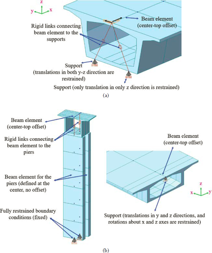
y and z directions were restrained, whereas in the second support, only the translations in the z direction were restrained. The provision of rigid links in a triangular fashion as shown in Figure 6-4(a) and the definition of boundary conditions as described previously provide the required torsional stability for the model. Several construction stages were defined as described in the load rating example to simulate the sequential nature of construction. The bridge constructed with the span-by-span method featured precast concrete segments. These segments were activated once their erection was completed.
For the bridge constructed with the balanced cantilever method, the piers were rigidly connected to the superstructure, as shown in Figure 6-4(b) (left), and roller supports were defined at the abutments, as shown in Figure 6-4(b) (right). Only one support point was defined at the abutments. For this support point, translations in y and z directions, and rotations about x and z axes were restrained. This created the required torsional stability in the model. Alternatively, the boundary conditions at the abutments could have been defined using the same approach used for the bridge constructed with the span-by-span method. Two rigid links were used to connect the piers to the reference nodes at the top of concrete segmental cross sections over the
piers. To accomplish this, the pier tables (i.e., the superstructure segments over the piers) were partitioned such that the reference nodes in the superstructure segments and those in the piers were in the same plane. The piers were fully restrained at the bottom. The concrete segments for the piers were defined using the centroid as the reference point. Several construction stages were created as described in the load rating example document to simulate the sequential nature of construction. The bridge constructed with the balanced cantilever method featured cast-in-place concrete segments. These segments were activated once the formwork was removed, and the post-tensioning forces were applied. The weight of wet concrete prior to formwork removal was considered to capture the time-dependent effects created by it.
In terms of the notional live load, both truck plus lane and tandem plus lane were considered initially. It was determined that the combination of truck plus lane controlled the load rating in the longitudinal direction. Therefore, the comparative analysis in the longitudinal direction was based on the combination of truck plus lane. Transformed-section properties were used when conducting load rating analysis. The influence of using gross-section properties is addressed in the subsequent sections.
Transverse Analysis
To conduct load rating analysis in the transverse direction, a 2D frame model that represents the segmental cross section was created. Pin and roller supports were located at the intersection of the web and bottom flange as shown in Figure 6-5. The locations of interest where flexural stress at service and flexural strength at the ultimate limit state were computed are illustrated in Figure 6-5 by the red circles. These locations include the root of the cantilever (Point 1), the intersection of the inside face of the web and top slab (Point 2), and the midspan of the top slab (Point 3). A flowchart that describes how the transverse analysis was conducted is presented in Figure 6-6. After the creation of the 2D frame model, all permanent loads, including transverse post-tensioning, were applied on a per-foot basis. Moment due to permanent loads and prestressing were determined at the critical locations.
Live load effects were quantified using Homberg (1968) influence surface charts, obtaining fixed end moments, applying these fixed end moments to the 2D frame, and calculating final moments by summing fixed end moments and distributed moments. The notional live load used to conduct load rating analysis in the transverse direction included the HL-93 design truck or tandem loading, whichever produced the worst-case effect. The influence of the presence of multiple trucks was evaluated by considering appropriate MPFs. The guidelines in AASHTO MBE (2018) were followed for the application of vehicular live load. Based on Article 6A.2.3.2 in AASHTO MBE (2018), the center of any wheel load shall not be closer than 2.0 ft from the edge of a traffic lane or face of the curb. In addition, the distance between the center of the wheels of two adjacent trucks should not be less than 4.0 ft.


Secondary prestressing effects and prestresses losses were considered. Secondary moments due to creep and shrinkage were considered; however, they were found to be too small to make an impact. Only one time step was considered to account for time-dependent effects, which was from completion of construction and opening of the bridge to traffic to 10,000 days. Temperature gradient effects were not included in the transverse analysis. Unlike the load rating analysis in the longitudinal direction, which to a certain extent was automated through the use of an algorithm created in Mathcad, load rating analysis in the transverse direction was conducted manually, when it came to the computation of stresses at service and the verification of shear and moment capacities for the top slab obtained from Midas Civil 2023.
6.4.3 Validation of Numerical Modeling Protocol in the Longitudinal Direction
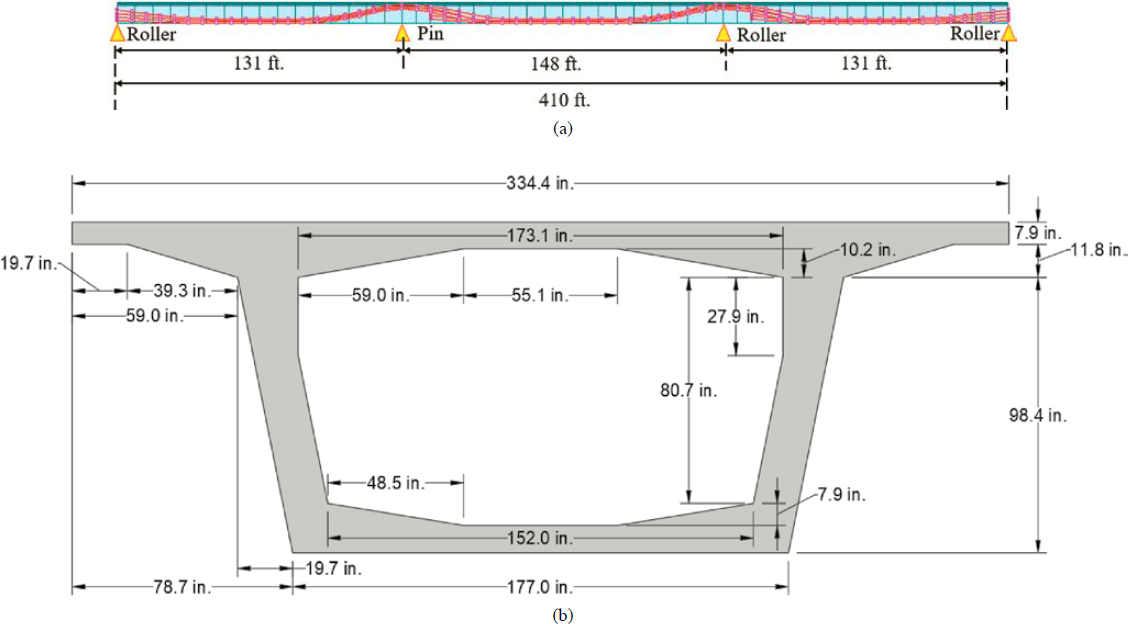
The numerical modeling protocol used in the longitudinal direction was validated by investigating the capability of Midas Civil 2023 to accurately simulate creep, shrinkage, and temperature effects based on a given input. The concrete segmental cross section shown in Figure 6-7 was used to conduct a comparison between theoretical and computed results. The section properties for this concrete segmental cross section are given in Table 6-7. The comparison was conducted between computed and predicted results. Predicted results were based on linear elastic engineering mechanics, and when creep effects were considered, they were based on viscoelastic analysis. Comparison with field data is presented in Section 6.4.7 with respect to live load induced strains in the transverse direction. Since long-term field data in the longitudinal direction included the combined effects of creep, shrinkage, uniform temperature, and temperature gradients, the validation of numerical loading protocol was conducted at the fundamental level between computed and predicted results for each effect independently.
6.4.3.1 Temperature Gradient
The concrete segmental cross section shown in Figure 6-7 was subjected to the positive temperature gradient specified for solar radiation zone 3 in AASHTO LRFD (2020a) as illustrated in Figure 6-8. Cross-sectional stresses calculated based on engineering mechanics were compared

Table 6-7. Section properties.
| Parameter | Value |
|---|---|
| Area, AG (in.2) | 5,808 |
| Moment of Inertia, IG (in.4) | 3.93 x 10⁶ |
| Concrete Compressive Strength, fc′, (ksi) | 7 |
| Modulus of Elasticity, EC, (ksi) | 4,770 |
| Coefficient of thermal expansion, α, (1/°F) | 6 x 10⁻⁶ |
| Centroid of the section measured from bottom, ybot, (in.) | 47.53 |
with those obtained from Midas Civil 2023. It was assumed that the segmental cross section existed in a simply supported beam configuration so that any stresses that were created due to temperature gradient applied at any given section along the span.
To conduct this comparison, piecewise linear functions were established to describe the variation of temperature gradient along the depth of the segmental cross section as shown in Figure 6-9. The top of the section was used as the reference point for defining the variable y (i.e., the variable y, which represents the distance from the top fiber, assumes a positive value


from the top fiber toward the bottom fiber as shown in Figure 6-9). Two piecewise functions are defined.
When the temperature gradient is multiplied by the coefficient of thermal expansion, free strains in the segmental cross sections may be obtained. When the free strains are multiplied by the modulus of elasticity, free stresses are obtained as follows.
| (6-6) |
It should be noted that the free strains mentioned cannot materialize because of the nonlinear nature of the temperature gradient and because plane sections before bending will tend to remain plane after bending. In other words, the tendency of each fiber to contract and expand freely is restrained by the adjacent fibers when the imposed strain distribution is nonlinear. The tendency to resist the creation of such free strains gives rise to the formation of restrained strains. If these restrained strains are further multiplied with the modulus of elasticity, restrained stresses, which are equal and opposite to the free stresses are obtained. These free stresses can be integrated to calculate the total axial force and bending moment in the segmental cross section as shown in Eq. (6-7) and Eq. (6-8), where F is the total axial force; M is the total bending moment; Ec is the modulus of elasticity of the concrete; α is the coefficient of thermal expansion; T(y) is the temperature gradient function previously defined; and b(y) is the width of the section as a function of section height.
| (6-7) |
| (6-8) |
Since the functions for temperature gradient are piecewise functions and not continuous ones, the integration is conducted in three parts from y = 0 to y = 4 in.; from y = 4 in. to y = 10 in.; and from y = 10 in. to y = 16 in. The parameter b(y) assumes a value of 336 in., 336 in., and 24 in. for each of the y intervals mentioned, respectively. The results of the integration are shown in Table 6-8 and Table 6-9. The total axial force and bending moment in the cross section are equal to and , respectively.
Table 6-8. Calculation of free axial force in the cross section.
| Part | y (in.) | b(y) (in.) | T(y) (in.) | Fi (kips) |
|---|---|---|---|---|
| 1 | 0 ≤ y ≤ 4 | 336 | 46 – 8.5y | F1 = 1115.5 |
| 2 | 4 < y ≤ 10 | 336 | 16 – y | F2 = 519.3 |
| 3 | 10 < y ≤ 16 | 24 | 16 – y | F3 = 12.4 |
Table 6-9. Calculation of free bending moment in the cross section at the top.
| Part | y (in.) | b(y) (in.) | T(y) (in.) | Mi (kips-in.) |
|---|---|---|---|---|
| 1 | 0 ≤ y ≤ 4 | 336 | 46 – 8.5y | M1 = 1795.1 |
| 2 | 4 < y ≤ 10 | 336 | 16 – y | M2 = 3461.9 |
| 3 | 10 < y ≤ 16 | 24 | 16 – y | F3 = 148.4 |
Final stresses in the cross section are calculated by superimposing the free stresses with the stresses created by the axial force and bending moment previously mentioned using the formula. This is illustrated in Figure 6-10. The stresses created due to the integrated axial force and bending moment were obtained using the formula P/A + My/I. It should be noted that the net stresses are self-equilibrating in nature, in the sense that if the net stress diagram were to be integrated along the segmental cross section, the net axial force and bending moment would be zero, since there are no externally applied forces. This check can be used to ensure that the calculations are conducted correctly. However, it should be noted that this check applies to simply supported configurations, where restrained axial forces and bending moments arising due to the statical
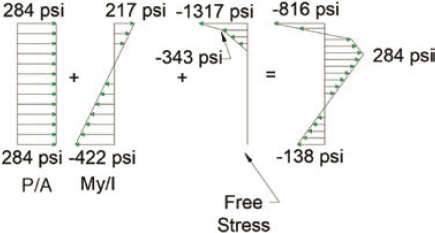
indeterminacy of the beam do not exist. For continuous beam superstructures, the integration of cross-sectional forces should equal the externally applied restrained forces. It is also worth noting that typically, in stress analyses that include temperature gradient, the gradient is assumed to form over a relatively short time (such as within 8 hours). Therefore, temperature gradient-induced creep effects are typically ignored. If the temperature gradient is sustained over a longer period, stresses created because of it will be relieved to a certain extent.
The self-equilibrating stresses mentioned were compared with those obtained from Midas Civil 2021 as shown in Figure 6-11. The results were identical, which shows that Midas Civil 2023 can compute stresses due to the defined temperature gradient accurately.
6.4.3.2 Creep
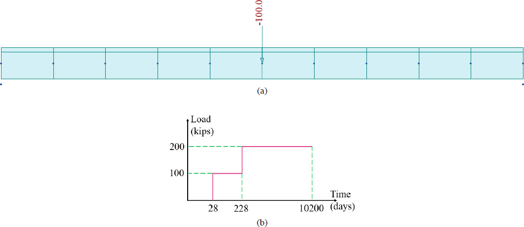
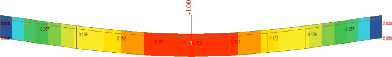
The concrete segmental cross section described in the previous section was used in the following problem to investigate the capabilities of Midas Civil 2023 to simulate creep effects. The segmental cross section was used in a simply supported beam configuration. The age of concrete was assumed to be 28 days and the modulus of elasticity was assumed to remain constant (i.e., no aging effect) and assumed a value of 4,770 ksi over the period considered in this exercise. It should be noted that while Midas Civil 2023 is capable of simulating the aging effects through the use of a time-varying modulus of elasticity, which is obtained based on a time-varying compressive strength function, the aging effect was ignored. A load of 100 kips was applied at the concrete age of 28 days and kept constant until 228 days. An additional 100 kip load was applied at the age of 228 days and kept constant until the age of 10,200 days. The elevation of the beam, the applied load, and the loading history are provided in Figure 6-12. The beam was assumed to be composed of plain concrete to directly investigate creep effects. Self-weight effects were ignored.
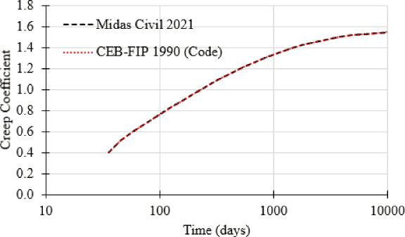
Creep effects at the material level were based on the CEB-FIP (1990) model. The relative humidity was assumed to be 70%. The type of the cement was assumed to be normal cement.

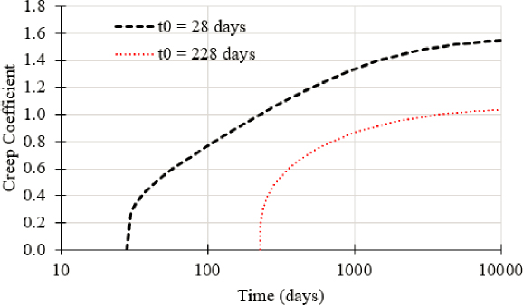
Only creep effects were examined (i.e., shrinkage was excluded to focus the validation on creep). The ability of Midas Civil to accurately simulate creep effects at the material level based on the specified model is illustrated in Figure 6-13, where the loading age was assumed to be 28 days. Since there are two loading events specified in the problem statement, two separate creep curves were used with loading ages of 28 days and 228 days, respectively. These two separate creep curves are illustrated in Figure 6-14.
Creep effects were calculated using the principle of superposition. The time-dependent strain at any concrete fiber can be calculated by summing the elastic and creep strains due to initial stresses, and elastic and creep strains due to changes in stress as shown in Eq. (6-9), where εt is total strain at time t; σ0, σ(τ) is stress at time t0 and τ, respectively; E0, E(τ) is modulus of elasticity at times t0 and τ, respectively; and φt,t0, φ(t, τ) is creep coefficient at time t due to load applied at time t0 and τ. The first expression (i.e., the one before the integral) represents the elastic and creep strains due to a stress applied at time t0. The second expression (the integral term) represents the elastic and creep strains due to changes in stress in the time interval t0 to t.
In this exercise, since the beam was simply supported, and consisted of plain concrete, there was no strain redistribution at the cross-sectional or member level, therefore, the second term did not apply. In the first expression, the ratio represents the initial elastic strain, represents the creep strain, and represents the total strain due to the initially applied loads.
| (6-9) |
Two time intervals were considered: (1) from 28 days to 228 days, and (2) from 228 days to 10,200 days. A total of three creep coefficients were obtained for these two time intervals to calculate creep deformations at each time step as shown where ϕ(t,t0) represents the creep coefficient at time t based on the loading age of t0 days. The creep coefficient represents the ratio of creep strain to the initial elastic stress-induced strain and can assume any value greater than zero.
The immediate deflection caused by the 100 kips applied at 28 days load can be calculated using the well-known formula for a simply supported beam loaded at midspan where P is the applied load; L is the beam length; E and I are the concrete modulus of elasticity and moment of inertia of the section, respectively. The immediate deflection is equal to 0.192 in. as shown in Eq. (6-10). The same immediate deflection would be obtained for the second concentrated load applied at 228 days since the modulus of elasticity was assumed to remain constant in this example. Figure 6-15 shows that the immediate deflection was calculated accurately by Midas Civil 2023.
| (6-10) |
Since the simply supported concrete segmental beam considered in this example was assumed to be composed of only concrete (i.e., no tendons) the additional creep deflection may be calculated using Eq. (6-11) and is directly proportional to the creep coefficient. It should be noted that this equation is only valid for plain concrete and assumes that compressive creep is equal to tensile creep (a common assumption in time-dependent structural analysis).
| (6-11) |
Creep strain can be further calculated as described in the Eq. (6-12), where εcc(t, t0) is the creep strain at time t due to the load applied at t0; ϕ(t, t0) is the creep coefficient at time t due to the load applied at t0; and Ec is the modulus of elasticity at 28 days, which needs to be determined based on the formula given in the relevant code (not the one defined under material properties in Midas Civil 2023).
| (6-12) |
In the CEB-FIP (1990) code, the modulus of elasticity of the concrete at 28 days was calculated based on the Eq. (6-13) where fc′ is the concrete compressive strength at 28 days, where fc′ and Ec are in MPa.
| (6-13) |
Midas Civil 2023 does not use the Ec value provided under material properties (4,770 ksi) but uses Eq. (6-13) for the calculation of the creep strain, and hence creep deformations. Immediate deflections were calculated based on the Ec value provided under material properties. Using the CEB-FIP (1990) code and assuming fc′ = 7 ksi concrete, the Ec value was calculated as follows.
| (6-14) |

In this example, the creep deformation was calculated as follows:
| (6-15) |
From t0 = 28 days to t1 = 228 days, the creep coefficient ϕ(228,28) was calculated as 0.998 as shown in Eq. (6-15). The creep deformation at the age of 228 days was expected to be 0.164 in. as shown in Eq. (6-16). This calculated creep strain from 28 days to 228 days was compared to that obtained from Midas Civil 2023. Figure 6-16 suggests that the calculated and computed creep deformations for this time step are identical. It should be noted that these deformations are those induced by creep only and do not include elastic deformations.
| (6-16) |
The total creep deflection between 228 days and 10,200 days can be calculated as shown in Eq. (6-17). This predicted creep deformation was compared with that obtained from Midas Civil 2023. Figure 6-17 suggests that the results are rather similar (0.262 in. calculated versus 0.258 in. computed, i.e., 1.5% error). Again, these deformations are those induced by creep only and do not include elastic deformations.
| (6-17) |
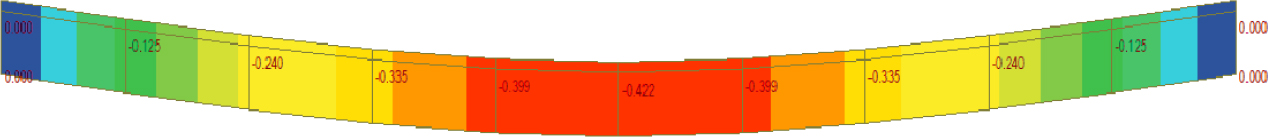
When the total creep deformations were considered, the calculated total creep deformation was equal to 0.426 in. as shown in Figure 6-18. The computed total creep deformation obtained from Midas Civil was equal to 0.422 in. (0.9% error).

| (6-18) |
The total calculated and computed deflections (immediate plus creep deflections) were compared in Table 6-10 for the three times considered in this example. Here, the deflections at 228 and 10,200 days were total deflections and included elastic as well as creep deflections. The ratio of computed to calculated deflections was 1.0 and the V was 0.4%, which suggests that Midas Civil 2023 is capable of predicting accurately creep effects.
6.4.3.3 Shrinkage
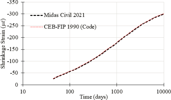
The simply supported concrete segmental beam mentioned previously was used to conduct a comparison between calculated and computed axial deformations due to a specified shrinkage strain. Since the beam was simply supported (i.e., pin supported on one end and roller supported at the other) it was subjected only to axial deformations and no stresses when subjected to uniform shrinkage. The specified shrinkage was based on CEB-FIP (1990). The ability of Midas Civil to predict shrinkage strains based on this model is illustrated in Figure 6-19. It was assumed that the beam was moist-cured for 28 days. The shrinkage strain at 10,200 days was calculated as −301 µε.
Considering that the beam length is 100 ft, the shrinkage-induced axial deformation at 10,200 days is 0.36 in. An identical axial deformation was computed by Midas Civil 2023 as shown in Figure 6-20.
| (6-19) |
6.4.3.4 Uniform Temperature Changes
The simply supported concrete segmental bridge mentioned previously was subjected to a uniform temperature change ∆T = +70 °F. The coefficient of thermal expansion was assumed
Table 6-10. Summary of the analysis results for creep deformation.
| Time (days) | Net Midspan Deflection (in.) | ||
|---|---|---|---|
| Theoretical deflection, ∆theoretical, (in.) | Midas Civil 2023 prediction, ∆Midas, (in.) | ||
| 28 | 0.192 | 0.192 | 1.00 |
| 228 | 0.548 | 0.548 | 1.00 |
| 10,200 | 0.810 | 0.806 | 0.99 |
| Average | 1.00 | ||
| St. Dev. | 0.00 | ||
| V (%) | 0.40 | ||

to be 6 p 10−6/°F. The axial elongation in the beam was calculated as 0.504 in. An identical axial elongation was predicted by Midas Civil 2023 as shown in Figure 6-21.
| (6-20) |
6.4.4 Comparative Analysis for a Concrete Segmental Bridge Constructed with the Span-by-Span Method
6.4.4.1 Description of the Bridge
The concrete segmental bridge used in the load rating example and constructed with the span-by-span method was used to conduct a comparative analysis. The elevation of the bridge and its cross section are shown in Figure 6-22. Detailed information about this bridge is provided in Appendix C of the Guideline.
6.4.4.2 Influence of Creep and Shrinkage Model on Load Rating
The influence of various creep and shrinkage models was investigated by load rating the abovementioned bridge several times based on different creep and shrinkage models. The considered models included (1) AASHTO LRFD (2020a), (2) FIB 2010, (3) CEB-FIP 1990, (4) CEB-FIP 1978,

and (5) ACI 209R.92. The load rating of the bridge was conducted at 10,000 days after the completion of construction and opening of the bridge to traffic. Figure 6-23 suggests that rating factors were mostly influenced by the service flexure limit state, in which the maximum percent change in rating factors was 9%, although the maximum change is noted for joints that are located in the vicinity of the second pier from the left. The controlling segment for this case was located at midspan of the second span. The percent change in the load rating factors for this segment for service flexure was less than 5%. These changes in rating factors could be impactful if the bridge was on the verge of a passing rating. The selection of creep and shrinkage models was less influential on the principal tensile stress limit state, in which the maximum percent change in rating factors was 3%. The impact of the selection of creep and shrinkage models was reduced further for the flexural strength limit state, in which the maximum percent change in rating factors was no greater than 1%. Similar observations were made for the shear strength limit state in which the maximum percent change in rating factors was 1.5%. While the selection of the creep and shrinkage models caused up to a 9% change in rating factors for service flexure, this change was much smaller than the change observed between the creep coefficients and shrinkage strains at the material level as illustrated in Figure 6-24. Concrete creep affected stresses at service through the variation of the prestressing force due to creep-induced prestress loss as well as through the development of creep-induced secondary moments, which were created as a result of stress redistribution. The use of various creep models results in some changes in top and bottom stresses caused by primary and secondary prestressing effects as well as secondary creep effects as shown in Figure 6-25. Top and bottom stresses were computed at 10,000 days. Although there was some variation in the stresses caused by secondary creep effects depending on each creep model chosen, this load case had a limited influence on net stresses at service. Figure 6-26 shows the variation of creep and shrinkage-induced prestress loss as a function of different models for three tendon groups (A1, B1, and C1). In this figure, the vertical black lines


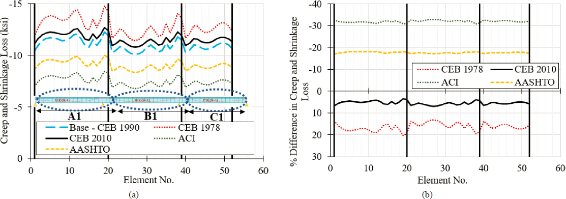
indicate the start and end locations of each tendon group. While there was some variation in creep and shrinkage-induced losses, this variation was smaller than 3.4 ksi at any given point when CEB-FIP 1990 is considered as a baseline. When considering the magnitude of the jacking stress as well as losses caused by other phenomena, this explains why the selection of creep and shrinkage models has a limited influence on stresses at service and consequently rating factors. Naturally, the time when the load rating was conducted affected the creep coefficient and shrinkage strain, and the reported differences in rating factors were a function of this time. However, despite a notable difference in the creep coefficients at 10,000 days, the change in rating factors was limited. Other conclusions were drawn for the bridge constructed with the balanced cantilever method. In addition, for the balanced cantilever bridge, the influence of rating time on load rating was examined.
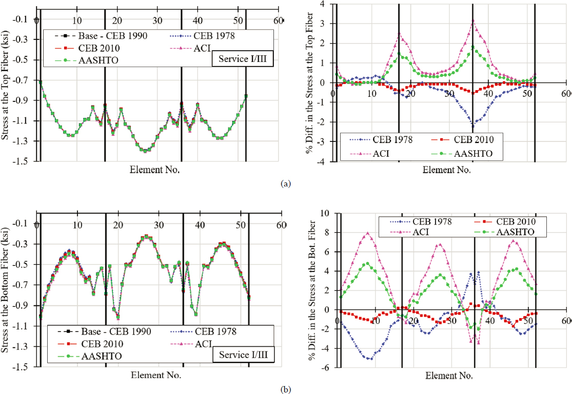
A separate evaluation was conducted to determine the impact of the selected creep and shrinkage model on stresses at service. Service I/III load combinations were used, such that if the live load created tension, the live load factor was taken as 0.80, otherwise it was taken as 1.0. Service I/III load combinations that featured positive and negative uniform temperature changes as well as positive and negative temperature gradients were considered, and the envelope values were used to examine the impact of creep and shrinkage model selection on service flexural stresses. Figure 6-27 illustrates this impact in terms of top and bottom fiber stress magnitudes as well as in terms of a percent change when the CEB MC 1990 model was used as the benchmark. The maximum percent difference in top and bottom fiber stresses is 3.2% and 8%, respectively. The maximum difference in top and bottom fiber stresses is 30 psi and 2 psi, respectively. Therefore, it can be concluded that the impact of creep and shrinkage model selection on stresses at service is minimal. A similar conclusion is presented in the commentary of AASHTO LRFD (2020a) Article C5.12.5.2.3.
6.4.4.3 Influence of Temperature Gradient on Load Rating
The consideration of temperature gradient in terms of its characterization and its impacts on cross-sectional stresses has been a source of controversy in the segmental bridge industry. Roberts-Wollmann et al. (2002) provide a good summary of some of the challenges associated with this load case, including a historical account of key changes related to this subject. AASHTO LRFD (2020a) Article C3.12.3 notes that “If experience has shown that neglecting temperature gradient in the design of a given type of structure has not lead to structural distress, the Owner
may choose to exclude temperature gradient.” Multibeam bridges are provided as an example for which judgment and experience should be considered.
Figure 6-28 shows the contribution of each load case in the computation of the bottom fiber stress in a segment located at midspan of the second span. The use of Service I (SRV I) load combination results in a net compression (0.02 ksi) (i.e., no tension) at the bottom fiber in the longitudinal direction. As expected, the load cases that created flexural tension in the bottom fiber were dead loads (DC and DW), secondary effects of prestressing (PSsc), and live loads (LL). The competing effects of primary and secondary prestressing forces are worth noting. The positive effects of primary prestressing were reduced to a certain extent by the secondary prestressing forces since the controlling segment was located at midspan. The ratio of dead load (DC+DW) induced bottom fiber stress to that induced by live load was 2.6.
The positive temperature gradient (TG) based on AASHTO LRFD (2020a) solar radiation zone III caused considerable flexural tensile stress at the bottom fiber (0.20 ksi). Tensile stresses caused by the positive temperature gradient were 74% of those caused by live load. While in this case, the inclusion of TG effects did not result in an inventory rating factor smaller than 1.0, the inclusion or exclusion of temperature gradient as a load case had a strong impact on the resulting rating factors. Figure 6-28(c) shows the distribution of cross-sectional stresses caused by the positive temperature gradient based on different solar radiation zones. Positive temperature gradient alone can create tensile stress in a considerable portion of the cross section,

although this is counterbalanced to a certain degree by the primary effect of prestressing. The magnitude and distribution of temperature gradient-induced stresses depend largely on the concrete segmental cross-sectional shape. It is worth noting in Figure 6-28(c–d) that the intensity of flexural stresses caused by temperature gradient varies as a function of the selected solar radiation zone with solar radiation zone 1 creating the largest flexural stresses and zone 4 creating the smallest ones. Therefore, when local reliable research-based data exist for the temperature gradient, such data may be used in lieu of AASHTO LRFD (2020a) prescribed temperature gradient to benefit load rating.
In terms of additional posting mitigation considerations, Corven Engineering (2004) provides the following discussion for longitudinal tension in epoxy joints. It is noted that because the bond usually exceeds the tensile strength of concrete in properly prepared epoxy joints, tensile stresses may be accepted as a function of the location and quality of the epoxy joint as follows:
- For top fiber stresses on the roadway surface, no tension is permitted for all load rating calculations.
- For bottom fiber stresses:
- Allow 0.2 ksi tension at good quality epoxy joints (i.e., no leaks and fully sealed).
- No tension allowed for poor quality epoxy joints (i.e., leaky or not filled gaps).
While these suggestions are presented in terms of additional posting mitigation considerations for longitudinal tension in epoxy joints caused by any load case, tension created by temperature gradients presents an example of when this avenue may be mobilized.
To further illustrate the impact that temperature gradient can have on stresses at service, the stresses caused by each load case on the top fiber are illustrated in Figure 6-28(b). In this case, the load combination considered included a positive temperature gradient, which created compression on the top. It is worth noting the compressive stress caused by temperature gradient is higher than that caused by dead loads. Since compressive stresses are typically not an issue, this is not a concern; it was illustrated here to highlight the potential of TG as a load case in terms of creating significant compressive and tensile stresses at service. When negative temperature gradients were considered, significant tensile stresses were created in the top fiber [Figure 6-28(d)], which may be more vulnerable to deterioration compared to the bottom fiber. However, these spikes in tensile stress apply only to a limited depth, which as noted previously, depends largely on the cross-sectional shape, and are temporary.
6.4.4.4 Influence of Compressive Strength Overstrength Factors on Load Rating
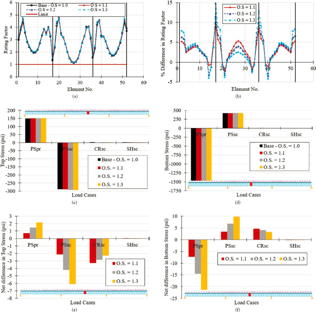
Figure 6-29 shows how the selection of a particular overstrength factor affects load rating. The rating factors in Figure 6-29(a) show the controlling factors for all limit states considered in the longitudinal direction (flexural stress at service, principal tensile stress in the web, flexural strength, and shear strength). A 30% increase in the overstrength factor results in up to a 15% increase in the controlling rating factor [Figure 6-29(b)]. Overstrength factors were applied to the compressive strength of concrete only at 28 days and their influence was considered in the structural analysis as well as in the capacity side. Overstrength strength factors were most impactful when considered in the capacity side at the service limit state since an increase in the specified concrete compressive strength resulted in an increase in the allowable flexural and principal tensile stress. Their influence on time-dependent structural analysis is illustrated in Figure 6-29(c–f) in terms of the top and fiber stress magnitude. The use of overstrength factors resulted in stronger concrete, which creeps less, and results in lower creep-induced prestress losses. This resulted in higher primary and secondary prestressing forces, which resulted in higher stresses. However, this increase was negligible [smaller than 2%, see Figure 6-29(e–f)]. The use of overstrength factors also resulted in smaller stresses caused by secondary creep effects with stronger concretes resulting in lower creep-induced stresses. However, the reduction in top and bottom fiber stresses caused by secondary creep effects was smaller than 6%.
6.4.4.5 Influence of Concrete Strength Development on Load Rating
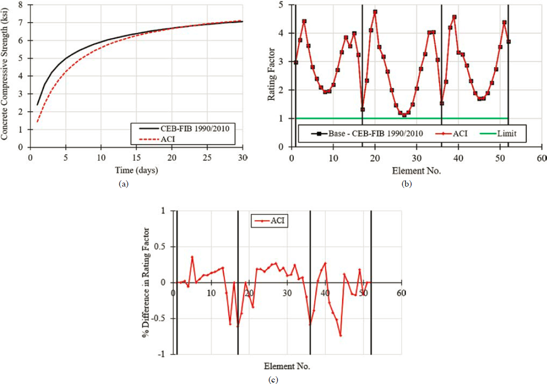
Figure 6-30(a–c) shows the influence of the predicted variation of compressive strength with time on load rating. Two models were used to predict the variation of compressive strength with time: the CEB-FIP 1990/fib 2010 model and the ACI 209R.92 (ACI 1992) model. For the ACI 209R.92 (ACI 1992) model the parameters (a) for cement type and (b) for curing method were taken as equal to 4 and 0.85, respectively. The CEB-FIP 1990 and fib 2010 models are identical provided that the aggregate factor is assumed to be 1.0 as was done in this case. The functions used to determine the variation of compressive strength with time were used to predict the variation of modulus of elasticity with time. The time-dependent modulus of elasticity was used to determine the effective modulus, which accounted for creep effects. While there was some variation in the predicted strength with time between the two models, this difference diminished after 15 days. The selection of one model or the other was inconsequential when it came to load rating, as the difference in load rating factors was negligible (i.e., smaller than 1%) [Figure 6-30(b–c)].
6.4.4.6 Influence of Various Load Cases on Principal Web Tensile Stress and Impact of Assumed Allowable Tensile Stress
In the analysis, the principal tensile stress check was conducted at all joints in the longitudinal direction. Along the depth of the segmental cross section, the principal tensile stress check was conducted at the centroidal axis. The evaluation of principal tensile stress at the centroidal axis was conducted because at this location shear stresses are highest. However, if the centroidal axis falls in the thickened portion of the web, then the check should be conducted at the critical elevation considering the coexistence of normal stresses. Similarly, if the centroidal axis (or critical elevation) falls within one duct diameter of the top or bottom of an internal, grouted duct, the web width for calculating stresses should be reduced by half the duct diameter (Corven Engineering 2004). When conducting the principal tensile stress check, concurrent vertical normal tensile stresses caused by transverse bending were ignored. Similarly, normal stresses caused by the temperature gradient were ignored.
Figure 6-31(a) shows the influence of each load case on the principal tensile stress calculated at the centroidal axis of a segment located over the interior support. Since the direction of principal tensile stresses caused by each load case was different, these stresses were not added algebraically to calculate a total principal tensile stress. Rather, an allowable shear stress was

calculated using Mohr’s circle by considering an allowable principal tensile stress ( = 0.25 ksi) as well as normal stresses caused by the prestressing effect. This allowable shear stress was then compared to shear stresses caused by each load case as shown in Figure 6-31(b), which also shows the summation of stresses caused by each load case based on Service III load combination. The rating of bridges that were controlled by the principal tensile stress was highly influenced by the adopted allowable tensile stress. Various allowable tensile stresses, ranging from to , were considered to show how the rating factor was influenced by the selected allowable tensile stress [Figure 6-31(c)]. Figure 6-31(d) shows the percent difference for the baseline case () and suggests that differences can be over 120%. The selected allowable tensile stress has a profound effect on rating factors. The allowable tensile stress depends highly on the assumed value for fc′. For load rating, fc′ may be based on actual compressive strength rather than specified compressive strength. When test data are not available, local research-based compressive strength overstrength factors may be used (Rizkalla et al. 2011; Rosa et al. 2007; Mante et al. 2019; Cakmak et al. 2022a, 2022b).
6.4.4.7 Influence of Condition Factors on Load Rating
A sensitivity analysis was conducted to determine how the selection of various condition factors affects load rating. The results are shown in Figure 6-32. A condition factor of 1.0 was selected to establish a baseline for comparisons. Two additional condition factors were considered: 0.85 and 1.10. The controlling rating factor pertains to flexural service stress at the 27th element, which is located at the midspan of the second span. Flexural service stress is a limit state not influenced by the selection of condition factors in the current formulation as it pertained to the service limit state (RF = 1.04). The lowest rating factors for flexural and shear strength in the longitudinal direction were 4.07 and 1.30, respectively.
Figure 6-32 suggests that condition factors have a strong influence on load rating; a 15% decrease in the condition factor caused up to a 42% decrease in the rating factors. Similarly, a 10% increase in the condition factors caused up to a 17% increase in the rating factors. For this example, the selection of various condition factors did not result in a change in the controlling limit state when flexural strength in the longitudinal direction is considered (i.e., even if a condition factor of 0.85 was chosen, the bridge still passes the load rating for longitudinal flexural strength with the lowest rating factor being 3.1), while the controlling load rating factor for service
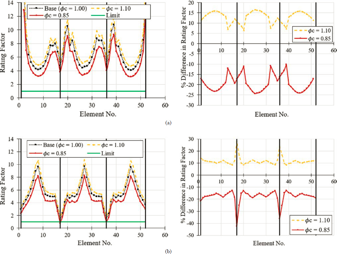
flexural stress is 1.04. However, the same is not true for vertical shear strength. When a condition factor of 0.85 is chosen, the load rating factor is reduced to a value smaller than 1.0 and becomes the controlling limit state (RF = 0.75).
Therefore, the current condition of the bridge as reflected through the use of a condition factor and thorough inspections greatly affects the rating of concrete segmental bridges. AASHTO MBE (2020) provides guidance for how to approximately convert superstructure condition ratings to equivalent member structural condition (Table C6A.4.2.3-1). The structural condition of the member can then be used to obtain a condition factor based on Table 6A.4.2.3-1. It is recommended that if the mode of deterioration is corrosion of tendons, and if section loss due to corrosion can be measured, the engineer should evaluate whether the fatigue life of the structure is affected. Two illustrative scenarios are outlined as examples. In the first scenario, a concrete segmental bridge experienced tendon corrosion. Although the extent of corrosion-induced section loss can be quantified, the structure shows no significant signs of distress, such as closed joints. Under these circumstances, the strength limit states should be evaluated based on the residual tendon cross section. While the service limit state related to flexural stress may remain unaffected, the prestressing stress of the remaining tendon cross section would increase due to force redistribution to maintain the original tendon force. The fatigue life of the prestressing tendons should be evaluated based on the increased service tendon stress. If the tendon stress fluctuates within the linear elastic range, the bridge will require an assessment for high cycle fatigue. In the second scenario, a concrete segmental bridge was subjected to tendon corrosion with measurable section loss and visible structural distress, such as open joints. In this scenario, the strength limit states must be reassessed based on the residual tendon cross section. It is probable that the bridge would not meet the service flexure, or possibly the principal tensile stress criteria either. Moreover, given that tendon stress likely surpassed the linear elastic threshold, the bridge should undergo an evaluation for low cycle fatigue.
In general, the use of condition factors must not be considered as a replacement for thorough inspections, or vice versa. Thorough inspections should be conducted and any measurable loss in tendon cross section or concrete segmental cross section, or any other type of deterioration should be included in the load rating calculations, including the consideration of additional limit states as discussed previously. The purpose of the condition factors, as noted in the AASHTO MBE (2020) is to account for the increased uncertainty in the behavior of a deteriorated bridge compared to that of an undeteriorated bridge.
6.4.4.8 Influence of Erection Time on Load Rating
The three-span concrete segmental bridge described in the load rating examples section was load rated one time assuming that two spans are erected each week, and another time assuming that one span is erected each week. The impact of erection time on rating factor is illustrated in Figure 6-33 for each of the limit states considered. The figures on the left show rating factor curves for each scenario, while the figures on the right show the percent change in rating factors using scenario 1 (i.e., two spans erected each week) as the benchmark. For this bridge, the impact of erection time on load rating factors was minimal. The maximum percent change did not exceed 0.8%, with the service flexure limit state being relatively the most sensitive. The change in erection speed affects the stress history in the concrete segments. However, since it was assumed that the segments were installed 28 days after fabrication, the impact of stress history on load rating factors was minimal. The small variations were a result of stress redistribution that took place due to time-dependent effects (such as creep). It should be noted that the focus of this evaluation was load rating. Separate evaluations should be conducted for the erection speed on erection stresses, deflections (which may cause unintended fitting problems), and so forth.
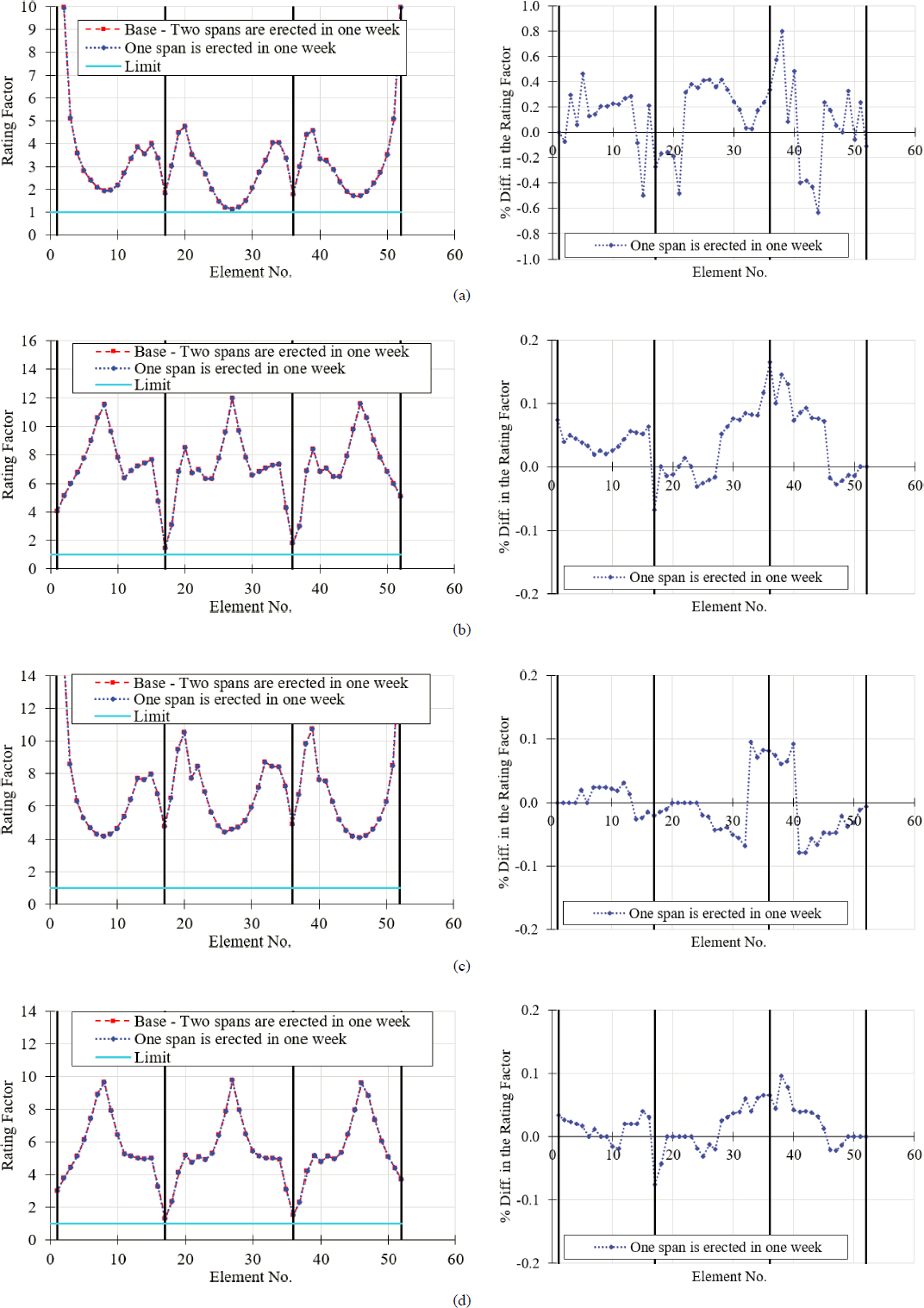
6.4.5 Comparative Analysis for a Concrete Segmental Bridge Constructed with the Balanced Cantilever Method
6.4.5.1 Description of the Bridge
The concrete segmental bridge used in the load rating example and constructed with the balanced cantilever method was used to conduct a comparative analysis. The focus of the comparative analysis is to understand how the selection of certain parameters affects the load rating of the bridge in the longitudinal direction. The goal of the analysis is to identify parameters that have a strong impact on load rating and those that do not. The elevation of the bridge and its cross section are shown in Figure 6-34. Detailed information about this bridge can be found in Appendix C of the Guideline.
6.4.5.2 Influence of Creep and Shrinkage Model on Load Rating
The influence of the creep and shrinkage models on load rating was investigated using various creep and shrinkage models. The considered models include (1) AASHTO LRFD (2020a), (2) fib 2010, (3) CEB-FIP 1990, (4) CEB-FIP 1978, and (5) ACI 209R.92. The load rating of the bridge

was conducted at 10,000 days after the completion of construction and opening of the bridge to traffic. The variations of creep coefficient and shrinkage strain are given in Figure 6-35(a–b). Since the cross section of the segments varies along the span, the first (i.e., deepest segment) was selected when creating Figure 6-35(a–b). In addition, the age of loading is considered as 5 days and the age of the segment when shrinkage starts to take place is assumed to be 3 days. As can be seen in Figure 6-35(a–b), the selection of the creep and shrinkage model has a strong impact on the development of the creep coefficient and shrinkage strain with time. It is interesting to note how certain models, such as CEB-FIP 1978, predict higher creep coefficients compared to the rest of the models, and lower shrinkage strains compared to most of the models. This results in higher prestressing losses due to creep and lower prestressing losses due to shrinkage. It is this canceling effect that dampens the impact that the selection of creep and shrinkage models has on load rating.
Figure 6-36(a–d) shows the effect of the creep and shrinkage model on load rating for different limit states. As can be seen in Figure 6-36(a), the selection of the creep and shrinkage model has a stronger impact on load rating for the flexural stress limit state compared to the bridge constructed with the span-by-span method. The maximum percent change in rating factors for service flexure is 20% compared to 9% as shown in the first example for the bridge constructed with the span-by-span method when the CEB-FIP 1990 model is considered as the benchmark. However, this maximum percent change in rating factors does not apply to the controlling segment, which is located near the right abutment as illustrated in Figure 6-37. For the controlling segment, the maximum percent change in the rating factors is 10%. The influence of the selected creep and shrinkage models remains somewhat notable for the principal tensile stress limit state, with the maximum percent change in the rating factors being as high as 12%. Unlike service flexure, this maximum percent change in rating factors takes place in the controlling segment. Similar to the observations made for the bridge constructed with the span-by-span method, the influence of the selected creep and shrinkage models is smaller for flexural strength and shear strength limit states. For flexural strength and shear strength limit states, the maximum percent change is less than 3% when the CEB-FIP 1990 model is considered as the benchmark. Therefore, it can be concluded that the selection of a creep and shrinkage model has a more profound effect on load rating for the service limit states than it does on the strength limit states.
Creep and shrinkage model selection affects load rating through the primary and secondary prestressing forces, which are a function of prestress losses, and through the magnitude of the
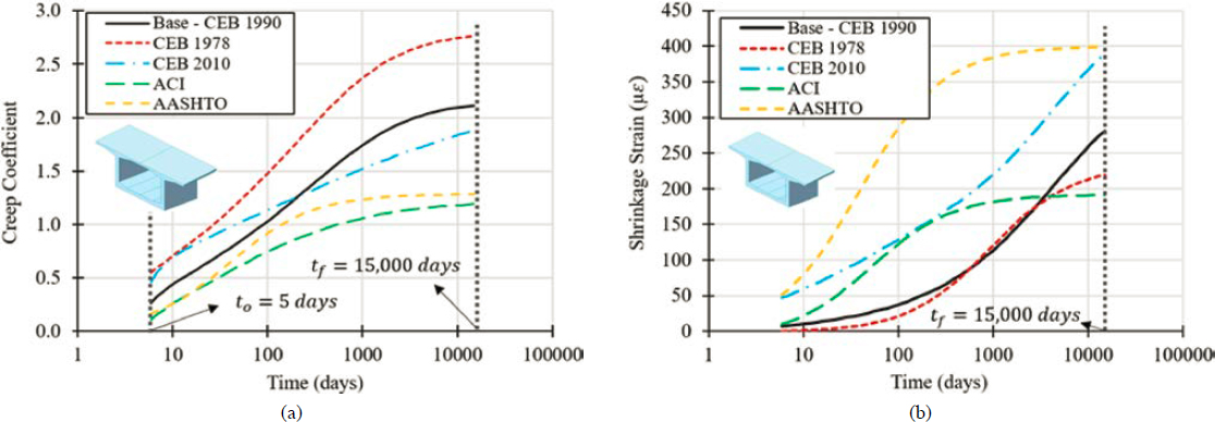
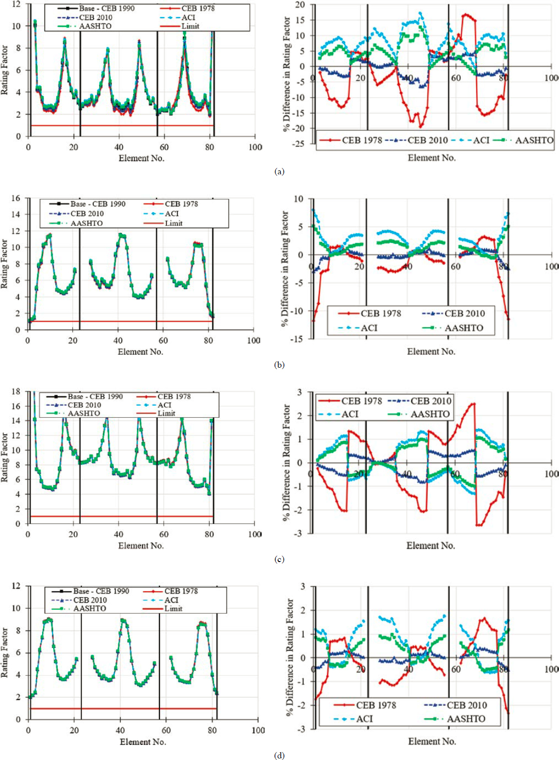
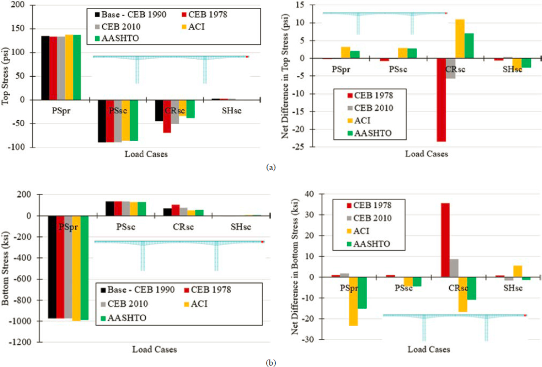
secondary forces due to creep and shrinkage. Therefore, to further understand how the selection of creep and shrinkage models influences load rating, their impact on the primary and secondary effects due to prestressing, creep, and shrinkage was investigated. This investigation was conducted for the flexural stress limit state in the longitudinal direction by computing top and bottom flexural stresses in the controlling segment. Figure 6-37 suggests that the variation of the primary and secondary prestressing forces as a function of the selected creep and shrinkage model is limited. This is perhaps due to the canceling effect of the higher creep coefficients and lower shrinkage strains that a particular model may have, as described previously. The variation in the creep and shrinkage-induced losses was investigated further as shown in Figure 6-38 for a strand group located over the first pier at 10,000 days. It should be noted that creep and shrinkage losses are presented together since the computation of both is based on a time-dependent strain compatibility analysis. Figure 6-38(a) suggests that in terms of prestress loss, the influence of creep and shrinkage models is limited to 8 ksi. In terms of percent change, the difference can be as high as 30%. The impact of the selected creep and shrinkage models on secondary creep forces is higher as shown in Figure 6-38(b). When all these effects are combined, the impact on load rating factors that the selection of creep and shrinkage models has is approximately 20%, when the CEB-FIP 1990 model is chosen as the benchmark. The difference in rating factors as a function of the selected creep and shrinkage models, also depends on the rating time. For a particular rating time, the relative difference in rating factors will impact changes in load rating factors. Unless there is reason to believe that one of the creep and shrinkage models allowed by AASHTO LRFD (2020a) is not appropriate, these models may be used for load rating to maintain the same level of flexibility provided in the design.
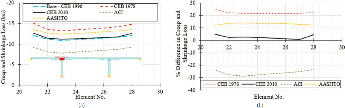
A similar evaluation was conducted for stresses at service to determine the impact of creep and shrinkage model selection on concrete segmental bridge design. Figure 6-39 shows the influence on service flexural stresses. Figure 6-39(a) (left) shows the variation of the top fiber stress as a function of location along the span and as a function of the selected creep and shrinkage model. Top fiber stresses are calculated at every joint along the span. Figure 6-39(a) (right) shows the percent difference in top fiber stress as a function of various creep and shrinkage models. Figure 6-39(b) (left) shows the variation of the bottom fiber stress as a function of location along the span, and Figure 6-39(b) (right) shows the percent difference in bottom fiber stress as a function of various creep and shrinkage models. The percent difference graphs are prepared by considering the CEB-FIP 1990 model as a benchmark model. Tensile stresses are positive and compressive stresses are negative. Some tension exists at the beginning and the end of the bridge near the abutments.
Service I/III load combinations are used such that if the live load created tension, the live load factor is taken as 0.80, otherwise the live load factor is taken as 1.0. There are a total of four load combinations for each fiber (top and bottom) due to the positive and negative uniform temperature changes and temperature gradient. The envelope values are presented in these figures. Figure 6-39(a) (right) suggests that there seems to be a maximum 30.7% difference in top fiber stresses when the CEB-FIP 1978 model is used as a benchmark. However, when the stress values are used as a metric for comparison, it can be seen that differences in service flexural stresses are small, that is, 0.026 ksi of tension for the CEB-FIP 1990 model and 0.018 ksi of tension for the CEB-FIP 1978 model (8 psi difference in tensile stresses). The high differences in terms of percent change are driven by the small benchmark value. Figure 6-39(b) (right) suggests that the maximum difference in terms of percent change in service flexural stresses at the bottom fiber is 19.1%. When a direct comparison of stress values is conducted, the maximum difference is determined when the CEB-FIP 1990 results in a flexural compressive stress of −0.968 ksi and the CEB-FIP 1978 model results in a flexural compressive stress of −0.783 ksi. In this case, the difference in service compressive stresses is higher, and it is equal to 185 psi. It is concluded that for this particular bridge, the impact of the selection of various creep and shrinkage models on service tensile stresses is small and limited to 8 psi, whereas the impact on service compressive stresses is higher and equal to 185 psi. Overall, considering the magnitude of allowable stresses at service the impact of the selected creep and shrinkage models in service flexural stresses

is limited. A similar conclusion is noted in the commentary of AASHTO LRFD (2020a) Article 5.12.5.2.3.
6.4.5.3 Influence of Temperature Gradient on Load Rating
The effect of various load cases and temperature gradients on load rating was investigated. The results are shown in Figure 6-40. Figure 6-40(a) and Figure 6-40(b) show the top and bottom flexural stresses, respectively, for the controlling segment in the longitudinal direction for Service I/III flexure. The controlling segment is located on the right-hand side of the cantilever of the second pier. This is because some of the bottom post-tensioning strands are discontinued at this location thus rendering this segment as the controlling segment. The primary and secondary prestressing forces have opposite effects on the controlling segment. The ratio of dead load (DC + DW) induced stress to live load-induced stress is 2.1.
The negative temperature gradient was the controlling gradient for this segment and its impact is shown in Figure 6-40(a) and Figure 6-40(b). The contribution of the negative temperature gradient to the bottom flexural stress is minimal because the tensile stress created because of it is small (0.01 ksi) as illustrated in Figure 6-40(a) and Figure 6-40(b). Conversely, the contribution of the negative temperature gradient to the top flexural stress is significant (0.27 ksi) when solar radiation zone III is considered. When the stresses due to each load case are
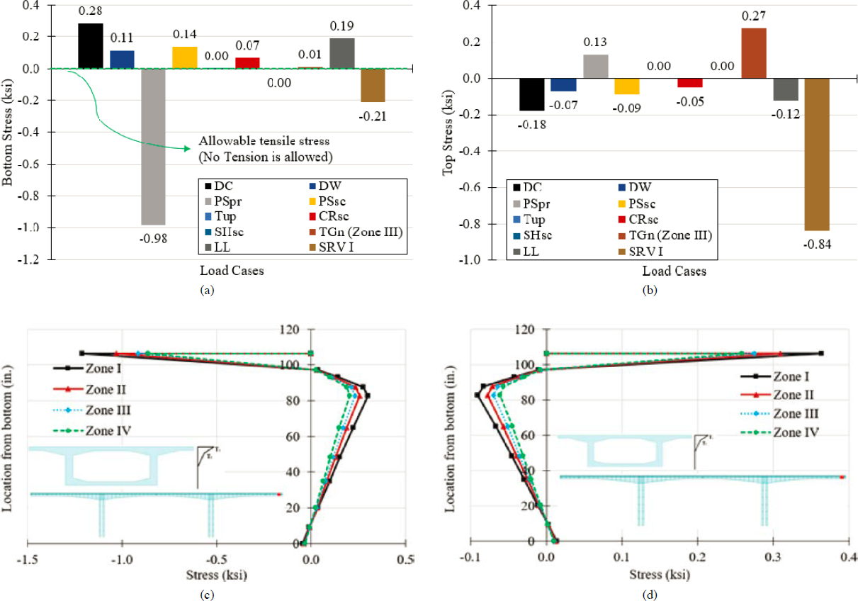
Figure 6-40. (a) Stress in the bottom fiber caused by various load cases, (b) stress in the top fiber caused by various load cases, (c) cross-sectional stress distribution due to positive temperature gradients, and (d) cross-sectional stress distribution caused by negative temperature gradient (considered segment shown in red in the inset bridge elevation).
combined using Service I load combination, there is a net compression of 0.21 ksi in the bottom fiber, and a net compression of 0.84 ksi in the top fiber. Figure 6-40(c) shows the influence of the positive temperature gradient on cross-sectional stresses, although, as indicated previously, the positive gradient was not the controlling gradient for this segment in question. The positive temperature gradient creates tensile stresses at 20 to 90 in. from the bottom of the cross section. As noted previously, the extent and magnitude of temperature gradient-induced stresses depends largely on the cross-sectional shape and dimensions. For example, the distribution of cross-sectional stresses in the concrete segmental cross section used for this bridge, is significantly different from that obtained for the bridge constructed with the span-by-span method. Note that the controlling segment in this case is located near the right abutment where secondary restraint forces developed due to the fixed pier superstructure connection do not apply. Therefore, differences in temperature gradient-induced stresses are entirely due to differences in the segmental cross sections.
6.4.5.4 Influence of Compressive Strength Overstrength Factors on Load Rating
The influence of the compressive strength overstrength (OS) factor, which herein is defined as the ratio of measured concrete compressive strength to the specified concrete compressive strength, on load rating is examined. The results are shown in Figure 6-41 for all limit states considered in the longitudinal direction (flexural stress at service, principal tensile stress in the web, flexural strength, and shear strength). As was done for the span-by-span bridge example, the overstrength factors were applied to the compressive strength of concrete only at 28 days and their influence was considered on the demand side (i.e., forces obtained from structural analysis) as well as on the capacity side. Overstrength strength factors were most impactful when considered on the capacity side at the service limit state since an increase in the specified concrete compressive strength results in an increase in the allowable flexural and principal tensile stress. A 30% increase in the overstrength factor results in up to a 45% increase in the controlling rating factor, which pertains to the limit state of flexural tensile stress at service [Figure 6-41(b)]. In addition, the influence overstrength factor on time-dependent structural analysis is illustrated in Figure 6-41(c-f) in terms of the top and bottom fiber stress magnitude. The use of overstrength factors results in stronger concrete, which creeps less, and results in lower creep-induced prestress losses. This results in higher primary and secondary prestressing forces, which result in higher stresses. However, this increase is negligible, that is, smaller than 12 psi. The use of overstrength factors also results in smaller stresses caused by secondary creep effects with stronger concretes resulting in lower creep-induced stresses. However, here again, the reduction in top and bottom fiber stresses caused by secondary creep effects is smaller than 4 psi.
6.4.5.5 Influence of Concrete Strength Development on Load Rating
The influence of the model that predicts the development of compressive strength with time on load rating was examined. The interest in this evaluation is the impact that the variation of compressive strength with time has on the variation of modulus of elasticity with time. The variation of modulus of elasticity with time is expressed using functions that depended on the variation of compressive strength with time. The variation of modulus of elasticity with time affected the calculation of transformed-section properties and the effective modulus, which captures creep effects. Two models were considered: (1) the CEB-FIP 1990/fib 2010 model, and (2) the ACI 209R-92 (ACI 1992) model. For the ACI 209R-92 (ACI 1992) model the parameters a for cement type and b for curing method were taken as equal to 4 and 0.85, respectively. The CEB-FIP 1990 and fib 2010 models are identical provided that the aggregate factor is 1.0. as was done in this case. Figure 6-42(a) shows the concrete compressive strength variation with time based on these two models. While there was some variation in the predicted strength with time between the two models, this difference diminishes after 15 days [Figure 6-42(a)]. The rating analysis results are shown in Figure 6-42(b) where all four limit states in the longitudinal directions are considered. The percent difference in the rating factor when the CEB-FIP 1990/fib 2010 model is considered as the benchmark is shown in Figure 6-42(c). As can be seen, the selection of one model or the other is inconsequential, as the difference in load rating factors is negligible (i.e., smaller than 2%.). Therefore, either model, ACI 209R-92 (ACI 1992) or the CEB-FIP 1990/fib 2010, may be used in the load rating of concrete segmental bridges to predict the variation of concrete compressive strength with time.
6.4.5.6 Influence of Various Load Cases on Principal Web Tensile Stress and Impact of Assumed Allowable Tensile Stress
The influence of load cases as well as allowable web tensile stresses was investigated for the concrete segmental bridge constructed with balanced cantilever method. The study was conducted for the controlling segment for principal web tension, which is the segment at
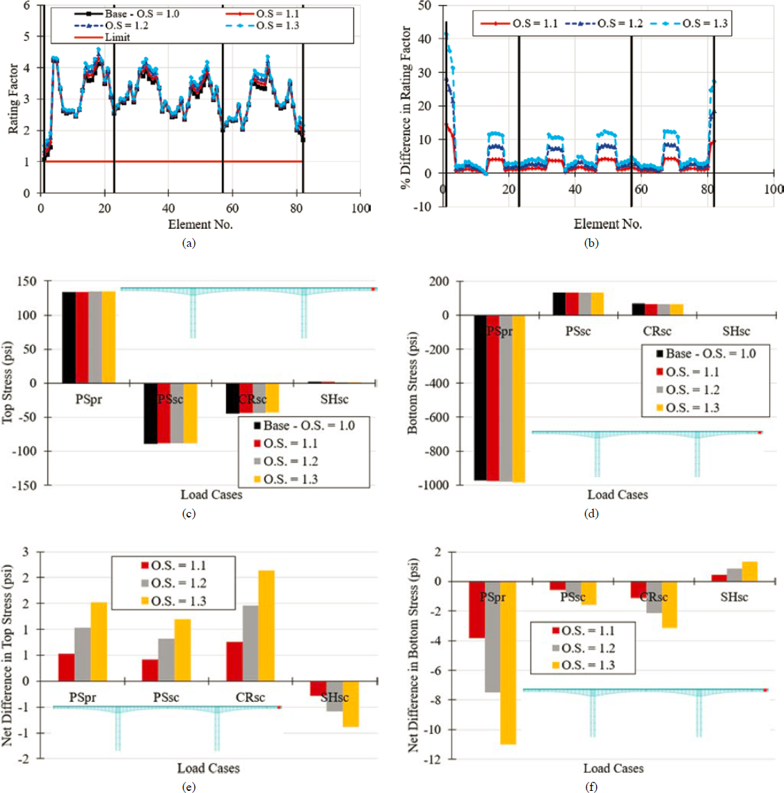

the first support (exterior support). The results are shown in Figure 6-43. Figure 6-43(a) and Figure 6-43(b) show the principal stresses and shear stresses caused by each load case, respectively. Figure 6-43(c) shows the variation of the rating factors as a function of the allowable tensile stress and Figure 6-43(d) shows the percent difference in the rating factors. The percent difference is calculated using as the benchmark allowable tensile stress. As can be seen, the selected allowable tensile stress causes a significant difference in the rating factors resulting in differences approaching 200%.
6.4.5.7 Influence of Condition Factors on Load Rating
The influence of condition factors on load rating in the longitudinal direction was investigated for the concrete segmental bridge constructed with the balanced cantilever method. The considered limit states include the flexure and shear strength limit since in the current formulation, condition factors influence only the strength limit states. Three condition factors were considered: 0.85, 1.0, and 1.10. The factor 1.0 was considered as the benchmark case. The factor 0.85 represents a deteriorated bridge, and the factor 1.10 represents a bridge constructed according to the New Directions for Florida Post-Tensioned Bridges (Corven Engineering 2004). Figure 6-44 suggests that the value assumed for the deterioration factor has a strong influence on load rating, assuming that the strength limit states control rating. A 10% increase in the condition factor
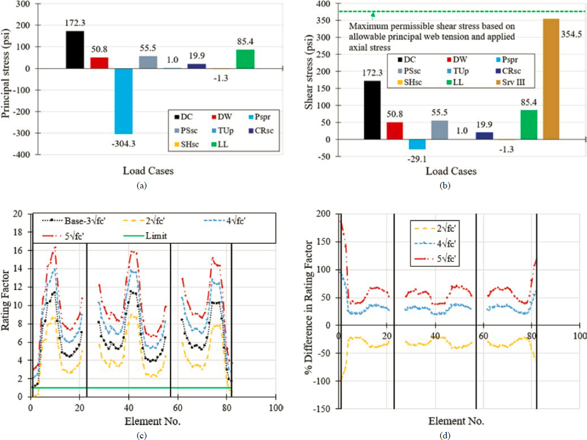
Figure 6-43. (a) Principal stress and (b) shear stress in a segment at the exterior support in a three-span concrete segmental bridge constructed with the balanced cantilever method, (c) rating factors based on principal tensile stress for all segments, and (d) difference in rating factors as a function of the allowable principal tensile stress.
results in up to a 20% increase in the rating factors. On the other hand, a 15% decrease in the condition factor results in up to a 32% decrease in the rating factors.
6.4.5.8 Influence of Final Analysis Time on Load Rating in Longitudinal Direction
The influence of the time when the bridge is rated on rating factors was investigated for the concrete segmental bridge constructed with the balanced cantilever method. The bridge was load rated at 5,000 days, 10,000 days, and 15,000 days after the completion of construction and opening of the bridge to traffic. The CEB-FIP 1990 model was used to predict creep and shrinkage effects. Load rating factors for each limit state in the longitudinal direction are shown in Figure 6-45. There is a general tendency toward smaller rating factors as the bridge gets older, simply due to the effect of time. The difference in rating factors when 10,000 days was considered as the
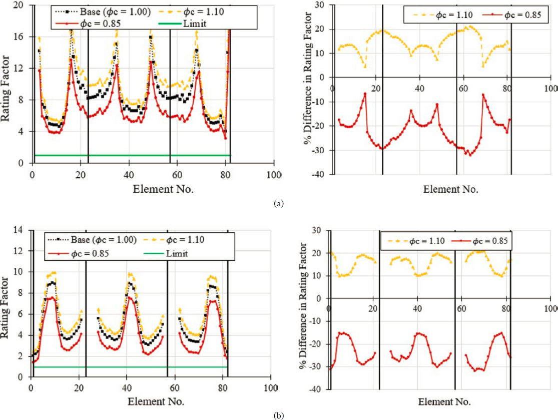
benchmark rating time were limited to 6% for the service flexure limit state. This difference is attributed solely to the time-dependent effects, since all other parameters were fixed and the only variable was the time when the bridge was rated. An examination of Figure 6-45 suggests that when the CEB-FIP 1990 model is considered, at 10,000 days, the majority of the concrete creep has taken place, whereas the shrinkage strain has not yet reached the ultimate value (the slope of the shrinkage curve is rather steep). Therefore, until all the creep and shrinkage in concrete and relaxation in strands take place, it is anticipated that there will be a reduction in rating factors solely due to an increase in prestress losses. Similarly, the higher the shrinkage, the higher the tensile stresses created by it due to the restraint provided by the piers. The influence of secondary prestressing effects depends on the segment under consideration. For some segments the secondary prestressing effects work against the primary prestressing effects, and for some others they have the same positive influence. Secondary creep effects will cause force redistribution such that forces and moment in some segments will increase and, in some others, will decrease.
The impact of rating time on the principal tensile stress limit state is limited to a 1.5% change in rating factors, that is, it is smaller than that noted for the service flexure limit state. The impact of rating time becomes even smaller for the strength limit states for which the maximum change in the rating factors is less than 0.5%.
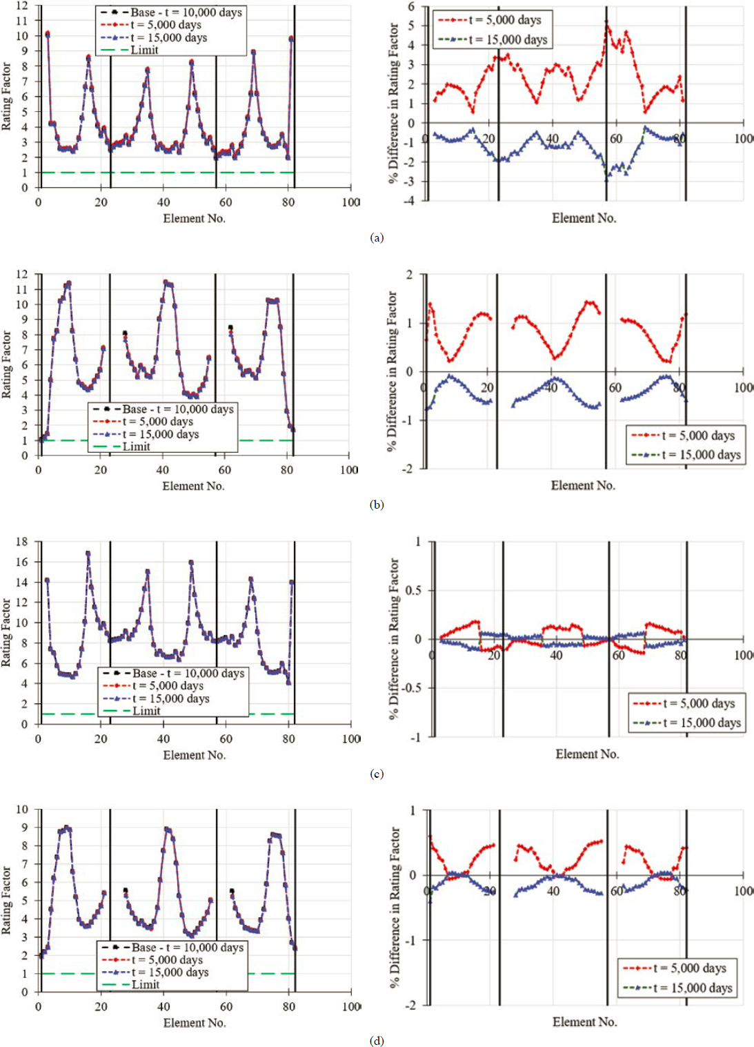
It can be concluded that the impact of the time when the bridge is rated depends on the time when the rating is conducted, the selection of the creep and shrinkage models, and the location of the section or joint that is being rated. The service flexure limit state is affected the most by the rating time followed by the principal tensile stress limit state. Ultimate strength limit states are barely influenced by the rating time for the cases considered in this study. Since general tendency is toward smaller rating factors as the bridge gets older, rating the bridge at initial and final ages when reviewing permit loads appears sufficient.
6.4.5.9 Influence of Gross- versus Transformed-Section Properties on Load Rating in Longitudinal Direction
The influence of the use of gross- versus transformed-section properties on load rating was investigated. In internally bonded concrete segmental bridge construction, initially, the self-weight of the segments and post-tensioning forces create stresses in the net cross section since the ducts are not yet grouted. After the grouting of the ducts, the application of subsequent loads, such as overlay, barriers, live loads, secondary effects (to a certain degree) causes stresses in the transformed cross section. In addition, the sequential nature of construction creates circumstances in which stresses are created in a partially grouted (i.e., partially transformed) cross section. The presence of these circumstances raises the question as to which cross-sectional properties would be appropriate for use in load rating. The concrete segmental bridge constructed with the balanced cantilever method was load rated one time using gross-section properties, and another time using transformed-section properties. When either gross or transformed-section properties were used, they were used for all load cases. The use of transformed-section properties included the transformation of reinforcement area into an equivalent concrete area. Other components, such as overlay and barrier were not included in this transformation and were considered only as loads.
The investigation was conducted for all limit states applicable in the longitudinal direction. The results are shown in Figure 6-46. The change in rating factors for service limit states is within 6.5%, and the change in rating factors for the strength limit state is limited to 1.5%. The limit state that was affected the most is service flexure, followed by principal web tension. The 1.5% change in the rating factors at the strength limit state is attributed to changes in the relative flexural stiffness of the different elements that compose the structure and the impact that flexural stiffness has on load distribution. The 6.5% difference in load rating factors may be capitalized on by the load rater when the bridge is on the verge of passing rating. The use of transformed-section properties should be reserved for load cases that justify their use (i.e., loads and deformations imposed after the grouting of the tendons).
6.4.5.10 Influence of Lane Configuration on Load Rating
The influence of lane configuration and multiple trucks was investigated by considering the concrete segmental cross section used in the balanced cantilever bridge load rating example. The configuration of the bridge used in the load rating example is shown in Figure 6-47. To investigate the influence of the number of lanes on load rating, the median barrier was removed, and the lane configuration was recreated such that the bridge features two lanes in Configuration 1 and three lanes in Configuration 2. For each configuration, the bridge was load rated multiple times to determine the controlling scenarios (i.e., single versus multiple lanes loaded) in the longitudinal and transverse directions. MPFs based on AASHTO LRFD (2020a) and AASHTO MBE (2018) were used when conducting this comparison. All ratings were conducted at the inventory level. Configuration 1 may be assumed to represent a scenario in which the bridge is load rated based on the number of striped lanes, and Configuration 2 may be assumed to represent a scenario in which the bridge is load rated based on the number of design lanes. It should be noted that when conducting the comparative analysis in the transverse direction, the notional live load was approached as close to the barrier as allowed by AASHTO MBE (2018) for both Configurations 1 and 2.
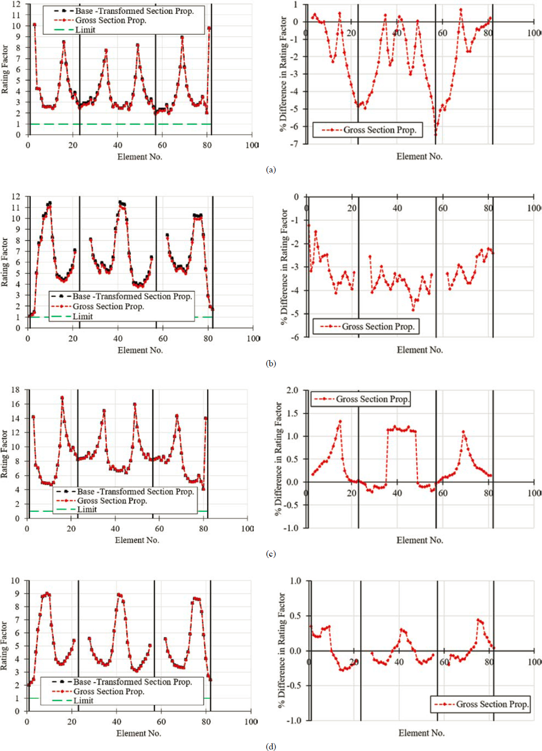

6.4.5.10.1 Comparative Analysis in the Longitudinal Direction
The results of the comparative analysis for Configurations 1 and 2 are shown in Table 6-11, Figure 6-48, Table 6-12, and Figure 6-49. Table 6-11 shows the summary of the comparative analysis in the longitudinal direction. Figure 6-48 shows the same information in a graphic format. Table 6-12 shows the ratio of Configuration 2 to Configuration 1 controlling rating factors. Figure 6-49 shows the variation of rating factors as a function of segment number in the longitudinal direction. The rating factors are shown for each limit state. In addition, Figure 6-49 shows the percent change in loading factor from Configuration 1 to Configuration 2. There is a consistent decrease of 22% in the rating factors when the lane configuration changes from Configuration 1 to Configuration 2 (i.e., from two lanes to three lanes). If we assume that Configuration 1 represents a striped lane scenario, and Configuration 2 represents a design lane scenario, there is a notable 22% decrease in the rating factors when the design lanes are
Table 6-11. Impact of lane configuration on load rating in the longitudinal direction.
| Limit State | Lane Conf. | Load Conf. | Number of Loaded Lanes | Element/Location | Rating Factor |
|---|---|---|---|---|---|
| Longitudinal Direction | |||||
| Flexure | Conf. 1 | Truck | 2 | 80 (3rd span near 2nd support) | 2.14 |
| Conf. 2 | Truck | 3 | 1.68 | ||
| Principal Web Tension | Conf. 1 | Truck | 2 | 1 (1st support) | 1.14 |
| Conf. 2 | Truck | 3 | 0.89 | ||
| Flexural Strength | Conf. 1 | Truck | 2 | 80 (3rd span near 2nd support) | 4.19 |
| Conf. 2 | Truck | 3 | 3.29 | ||
| Web Shear Strength | Conf. 1 | Truck | 2 | 1 (1st support) | 2.07 |
| Conf. 2 | Truck | 3 | 1.62 | ||
Conf. = Configuration.
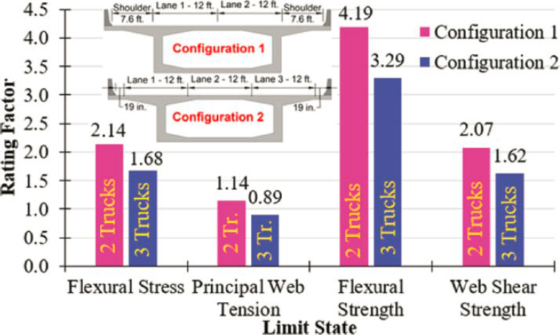
considered. The controlling scenario was when all three lanes are loaded. The reduction in the MPF of 15% cannot overcome the increase in the live load magnitude of 50% when switching from a two-lane configuration to a three-lane configuration. Within Configuration 2, the controlling case was when all three lanes are loaded. It should be noted that the element that controlled the load rating for each limit state did not change when switching from Configuration 1 to Configuration 2.
6.4.5.10.2 Comparative Analysis in the Transverse Direction
A similar comparison to that conducted in the longitudinal direction was conducted in the transverse direction with the purpose of determining the impact that lane configuration had on load rating. To conduct this comparison, the concrete segmental cross section located at midspan of the second span was considered because it features the shallowest depth. The selection of the shallowest versus the deepest section leads to more conservative results for negative moment regions at the inside face of the web, and less conservative results for the positive moment region at midspan of the top slab. These differences stem from the relative stiffnesses of the top slab, web, and bottom slab in the shallow and deep configurations. Corven Engineering (2004)
Table 6-12. Ratio of Configuration 2 to Configuration 1 controlling rating factors.
| Limit State | Rating Factor | Ratio: | |
|---|---|---|---|
| Conf. 1 (RF1) | Conf. 2 (RF2) | ||
| Longitudinal Direction | |||
| Flexure | 2.14 | 1.68 | 0.79 |
| Principal Web Tension | 1.14 | 0.89 | 0.78 |
| Flexural Strength | 4.19 | 3.29 | 0.79 |
| Web Shear Strength | 2.07 | 1.62 | 0.78 |
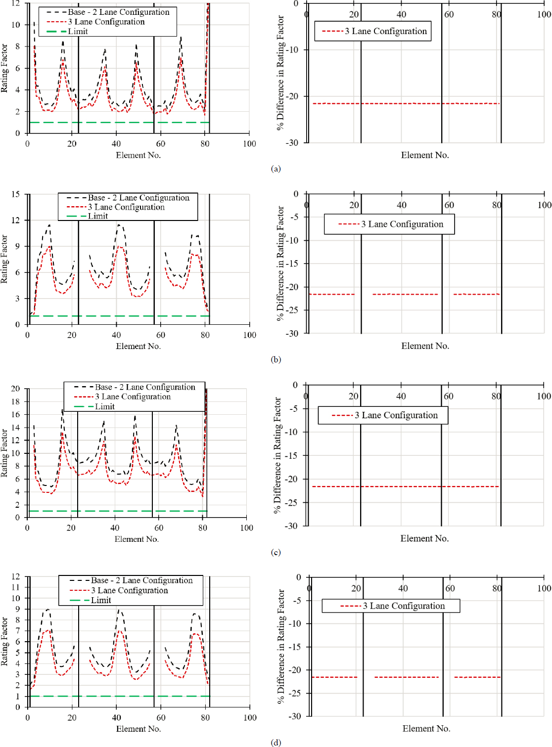
recommends that for load rating in the transverse direction, the cross section selected for load rating be that at midspan (i.e., the shallowest section). It is further noted that this approach is warranted to ensure the adequacy of cover concrete required as an essential part of the corrosion protection for cantilever and transverse post-tensioning.
The results of the comparative analysis in the transverse direction are shown in Table 6-13, Figure 6-50, and Table 6-14. Table 6-13 provides a summary of the comparative analysis. Figure 6-50 provides the same information in a graphic format. Table 6-14 provides the ratios of Configuration 2 to Configuration 1 controlling rating factors. As shown in Table 6-13, the controlling location changes when the lane configuration is switched from Configuration 1 to Configuration 2. For example, for top slab flexural stress at service, for Configuration 1, the controlling section is the midspan of the top slab, whereas for Configuration 2 it is the root of the cantilever. This is different from what was shown for the longitudinal direction in which the controlling segment and its location did not change when the lane configuration was changed from Configuration 1 to Configuration 2. Similarly, for the limit state of top slab flexural strength, the controlling location for Configuration 1 is the midspan of the top slab, and for Configuration 2, is the root of the cantilever. The controlling location for both limit states in the transverse direction did not change within the same lane configuration.
It is interesting to note, as demonstrated in Table 6-14, that there is no clear trend in terms of which configuration controls rating in the transverse direction. For two of the locations considered, both configurations resulted in identical rating factors. For two other locations, Configuration 1 controlled, and for the remaining two locations, Configuration 2 controlled.
6.4.5.11 Influence of Resal Effect
The influence of Resal effect on load rating was investigated for the limit state of vertical shear at the ultimate load level. The shear strength of non-prismatic concrete segments that feature an inclined bottom flange may be increased by considering the vertical component of the inclined compressive forces present in the bottom flange when the section is subject to a negative bending moment. The Resal effect is illustrated in Figure 6-51.
Table 6-13. Impact of lane configuration on load rating in the transverse direction.
| Limit State | Lane Conf. | Load Conf. | Number of Loaded Lanes | Location | Rating Factor |
|---|---|---|---|---|---|
| Transverse Direction | |||||
| Top Slab Flexure | Conf. 1 | Tandem | 1 | Root of cantilever | 1.66 |
| Truck | 2 | Left of top slab | 2.66 | ||
| Tandem | 2 | Midspan of top s. | 1.50 | ||
| Conf. 2 | Tandem | 1 | Root of cantilever | 1.66 | |
| Tandem | 2 | Left of top slab | 2.62 | ||
| Tandem | 1 | Midspan of top s. | 2.30 | ||
| Flexural Strength | Conf. 1 | Tandem | 1 | Root of cantilever | 2.20 |
| Truck | 2 | Left of top slab | 2.46 | ||
| Tandem | 2 | Midspan of top s. | 2.17 | ||
| Conf. 2 | Tandem | 1 | Root of cantilever | 2.20 | |
| Tandem | 2 | Left of top slab | 2.42 | ||
| Tandem | 1 | Midspan of top s. | 3.34 | ||
| Bold cells represent the governing rating factor and corresponding location. | |||||
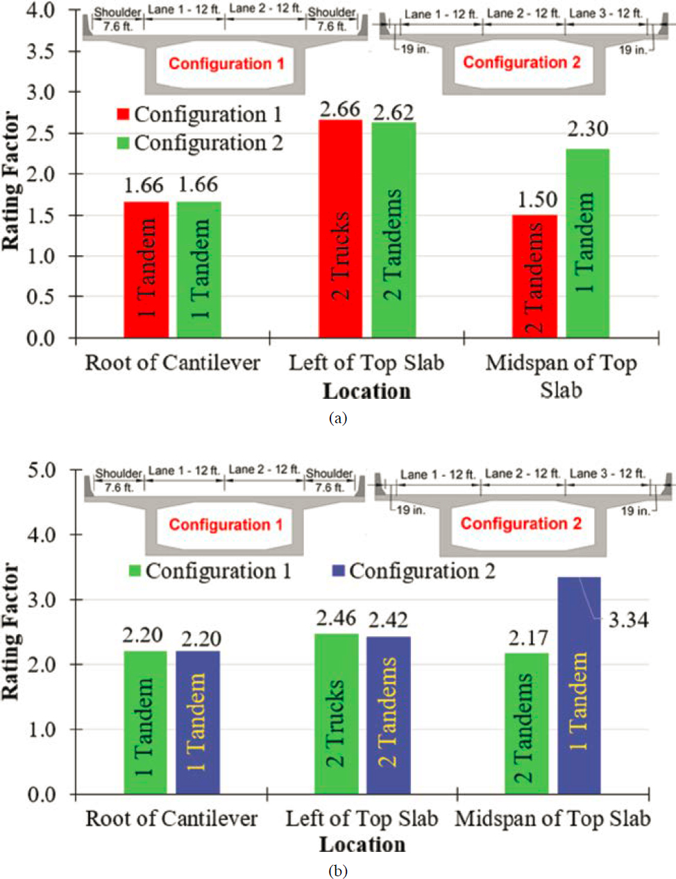
Table 6-14. Summary of the rating results based on lane Configurations 1 and 2.
| Limit State | Rating Factor | Ratio: | ||
|---|---|---|---|---|
| Conf. 1 (RF1) | Conf. 2 (RF2) | |||
| Transverse Direction | ||||
| Top Slab Flexure | Root of cantilever | 1.66 | 1.66 | 1.00 |
| Left of top slab | 2.66 | 2.62 | 0.98 | |
| Midspan of top slab | 1.50 | 2.30 | 1.53 | |
| Flexural Strength | Root of cantilever | 2.20 | 2.20 | 1.00 |
| Left of top slab | 2.46 | 2.42 | 0.98 | |
| Midspan of top slab | 2.17 | 3.34 | 1.54 | |
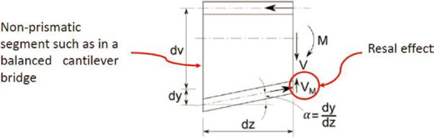
Figure 6-51. Illustration of the Resal effect.
The vertical component of the inclined compressive force in the bottom flange may be calculated as shown in Eqs. (6-21 through 6-23), where VResal is the additional shear resistance provided by the Resal effect; M is the unfactored negative moment at the section in question when maximum shear is obtained; α is the angle of inclination of the bottom flange with respect to the longitudinal axis; dv is the effective shear depth taken as the distance, measured perpendicular to the neutral axis, between the resultants of the tensile and compressive forces due to flexure [based on AASHTO LRFD (2020a) Article 5.7.2.8]; Mn is the nominal moment capacity of the section in question; de is the effective depth for bending (equal to dp in this case, because there is no non-prestressed reinforcement where dp is the effective depth of the prestressed strands); h is the section depth; As and fy are the area and yield strength of non-prestressed reinforcement (0 in this case because there is no non-prestressed reinforcement); Aps and fps are the area of the strand and strand stress at ultimate, respectively. The method presented previously is an approximation for calculating the Resal effect. In this approach, VM is a function of M where a concentric prestressing force will also induce VM in the bottom flange. This effect is ignored. In addition, the neutral axis may fall in the web rather than in the bottom flange when the section is subjected to negative moment. Since the inclination of the flange and that of the web is different, an angle different from α may need to be calculated if a higher level of accuracy is desired. This can be accomplished by considering the stress field for an infinitesimal element and determining the resultant compressive force together with its orientation.
| (6-21) |
| (6-22) |
| (6-23) |
To demonstrate the influence of the Resal effect on load rating for the shear strength limit state, the first span of the concrete segmental bridge constructed with balanced cantilever method is selected. When the bridge was modeled, a second-degree polynomial was used to describe the variation of the section depth along the span. The tapering starts after the I end of the 10th segment, as shown in Figure 6-52(a), meaning that the segment depths for elements No. 1 to 10 are the same. Considering the top of the I end of the 10th segment as the origin, the equation of the centroid of the bottom chord of the segments can be derived by using the known segment depths at the beginning and at the end of the span as follows where both y and x are in inches:
| (6-24) |
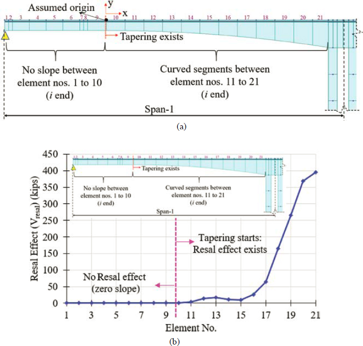
The first derivative of this function with respect to x provides the slope [or inclination: tan(α)] of the centroid of the bottom chord.
| (6-25) |
Since there is no slope for elements No. 1 and 10, the tan(α) = 0. It should also be noted that the x value provided in these equations should be based on the origin shown in Figure 6-52(a). When calculating the effective shear depth, dv, the necessary data were imported from Midas Civil 2023 at each joint, such as Mn, dp, Aps, and fps. Then, the dv values were calculated at each joint in Microsoft Excel. Similarly, the corresponding moment values in a segment caused by several load components when the shear was maximum were obtained from Midas Civil 2023. Since the load components caused by uniform and non-uniform temperature loads are not considered for the calculation of shear demand for the load rating calculation for the shear strength limit state, these are also not considered when calculating the total corresponding moment. In addition, no load factors were used when obtaining moment for each load case. After the locations of each joint with respect to the origin were determined, the vertical component of the inclined compression force at the bottom flange is calculated. The magnitude of this vertical component (i.e., the contribution of the Resal effect to shear strength) as a function of element number is illustrated in Figure 6-52(b). As expected, the segments that featured a bottom flange with zero slope with respect to the longitudinal axis are unaffected by the Resal effect. Resal effect becomes more pronounced toward the support as the slope of the bottom flange increases.
Having determined the shear force caused by the Resal effect, the load rating analysis for the shear strength limit state is repeated and the obtained rating factors are compared with those previously obtained by ignoring the Resal effect. The results are shown in Figure 6-53. As can be seen, while there is no change in the rating factor for elements No. 1-10, as evinced by the overlapping curves, the Resal effect becomes evident especially for elements No. 17-21, which feature higher rating factors when the Resal effect is included. The increase in rating factor is up to 11.4%. While for this particular bridge, the limit state of vertical shear at the ultimate load level was not the controlling limit state, the inclusion of the Resal effect may be used to benefit rating as an additional posting mitigation consideration tool for bridges controlled by this limit state. On the other hand, negative Resal effects must be included. This scenario is present in constant depth boxes with variable thickness in the bottom flange.
6.4.6 Impact of Multiple Trucks
The impact of multiple trucks on load rating of concrete segmental bridges was investigated by summarizing the results of the three load rating examples, which address bridges constructed with (1) the span-by-span method, (2) balanced cantilever method, and (3) incremental launching method. The goal was to determine which notional live load configuration controlled the rating of these bridges in the longitudinal and transverse directions. All three bridges feature two lanes. The summary of the load rating analysis for these three bridges is shown in Table 6-15. This summary includes the rating factors for each limit state in the longitudinal and transverse directions, the controlling segment or location, the controlling lane configuration, and the controlling live load configuration.
With respect to load rating in the longitudinal direction, a fully loaded bridge (i.e., two-lane loaded in these cases) controlled over a one-lane loaded bridge. While the one-lane loading case creates torsion in all three bridges, the two-lane loaded case with no torsion controlled. In addition, the combination of truck plus lane controlled over the combination of tandem plus lane.
With respect to load rating in the transverse direction, for the bridges constructed with the balanced cantilever method and incremental launching, the one-lane loaded configuration with tandem as the notional live load controlled over the two-lane loaded configuration. The controlling location for these two bridges was always the root of the cantilever for the service and ultimate limit states. For the bridge constructed with the span-by-span method, two-lane loaded configuration with the tandem as the notional live load controlled over the one-lane loaded configuration for the service limit state. The controlling location was the midspan of the top slab. For the ultimate limit state, for this bridge, the one-lane loaded configuration with truck as the notional live load controlled over the two-lane loaded configuration with the root of the cantilever being the controlling location. Generally, for the considered bridges, it was the one-lane loaded configuration that controlled the rating with the tandem as the notional live load and the root of the cantilever as the controlling location.
6.4.7 Comparative Analysis in the Transverse Direction
6.4.7.1 Introduction
A comparative analysis for the live load effects in the transverse direction between various analytical techniques was conducted for the Seabreeze Bridge located in Daytona, Florida. The live load effect in the transverse direction was quantified via live load testing in the field by Maguire et al. (2015). The measured strains due to live load were compared with those obtained using Homberg charts and a 2D frame model as well as those predicted by a 3D shell finite element
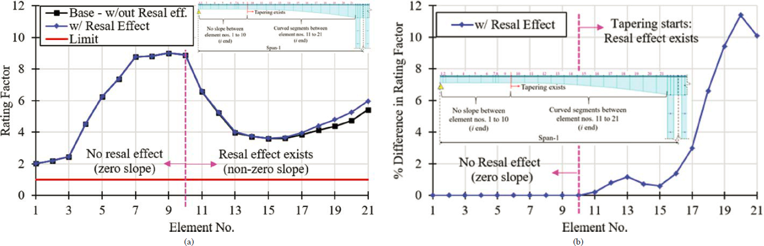
Table 6-15. Influence of multiple presence effects.
| No. of Lanes | Direction | Limit State | RF | Controlling Segment/Location | Controlling Case | Loading Conf. |
|---|---|---|---|---|---|---|
| Concrete Segmental Bridge Constructed with Span-by-Span Method | ||||||
| 2 | Longitudinal | Service—Flexure | 1.04 | 27 (Midspan of 2nd span) | Two-lane loaded | Truck |
| Service—Principal Tensile Stress | 1.45 | 17 (2nd support) | Two-lane loaded | Truck | ||
| Ultimate—Flexure | 4.07 | 46 (Midspan of 3rd span) | Two-lane loaded | Truck | ||
| Ultimate—Shear and Torsion | 1.30 | 17 (2nd support) | Two-lane loaded | Truck | ||
| Transverse | Service—Flexure | 2.44 | Midspan of top slab | Two-lane loaded | Tandem | |
| Ultimate—Flexure | 3.37 | Root of cantilever | One-lane loaded | Truck | ||
| Concrete Segmental Bridge Constructed with the Balanced Cantilever Method | ||||||
| 2 | Longitudinal | Service—Flexure | 2.02 | 80 (3rd span near 2nd support) | Two-lane loaded | Truck |
| Service—Principal Tensile Stress | 1.06 | 1 (1st support) | Two-lane loaded | Truck | ||
| Ultimate—Flexure | 4.07 | 80 (3rd span near 2nd support) | Two-lane loaded | Truck | ||
| Ultimate—Shear and Torsion | 2.00 | 1 (1st support) | Two-lane loaded | Truck | ||
| Transverse | Service—Flexure | 1.66 | Root of cantilever | One-lane loaded | Tandem | |
| Ultimate—Flexure | 2.20 | Root of cantilever | One-lane loaded | Tandem | ||
| Concrete Segmental Bridge Constructed with the Incremental Launching Method | ||||||
| 2 | Longitudinal | Service—Flexure | 2.76 | 24 (Midspan of 1st span) | Two-lane loaded | Truck |
| Service—Principal Tensile Stress | 2.46 | 55 (3rd support) | Two-lane loaded | Truck | ||
| Ultimate—Flexure | 4.13 | 66 (Midspan of 3rd span) | Two-lane loaded | Truck | ||
| Ultimate—Shear and Torsion | 1.33 | 55 (3rd support) | Two-lane loaded | Truck | ||
| Transverse | Service—Flexure | 1.17 | Root of cantilever | One-lane loaded | Tandem | |
| Ultimate—Flexure | 1.40 | Root of cantilever | One-lane loaded | Tandem | ||
analysis. The goal of the comparative analysis was to evaluate the accuracy of each analytical method and to make recommendations as to which analytical method would be appropriate for use in the load rating of concrete segmental bridges.
6.4.7.2 Field Data
The Seabreeze Bridge is a 10-span continuous precast, partially curved horizontally, concrete segmental bridge constructed with the balanced cantilever method. The cross-sectional
dimensions and a portion of the span where the strain gauges were located are shown in Figure 6-54. The instrumentation used by Maguire et al. (2015) featured strain gauges placed in the longitudinal and transverse directions. Since the focus of the analysis was to conduct a comparison of live load effects in the transverse direction, only data obtained from strain gauges installed in the transverse direction were considered. The location of these strain gauges is illustrated with the red circles in Figure 6-55 for Sections A and C, which are denoted in the partial elevation of the bridge superstructure in Figure 6-54.
The axle weights, truck dimensions, and truck positions used during the live load testing and considered in this comparative analysis are shown in Figure 6-56. Comparison of live loads effects is conducted for Sections A and C and for truck positions LC1, LC3, and LC4.
6.4.7.3 Analysis Using Homberg Charts and a 2D Frame Model
The 2D frame analysis in the transverse direction was conducted as described in Appendix C of the Guideline. Homberg charts were used to quantify live loads effects in terms of fixed end moments, which were then distributed to the 2D frame to obtain final moments. The boundary conditions featured pin and roller supports at the intersection of bottom flange and webs. The use of such boundary conditions and the combination of a 2D frame model with influence surfaces (Homberg charts) do not accurately represent the distortional effects that take place in the 3D structure. However, the use of 2D frame models and influence surfaces is a common first step in the design and evaluation of concrete segmental bridges.
6.4.7.4 3D Shell Finite Element Analysis
A partial 3D model of the superstructure of the Seabreeze Bridge was created in the commercially available finite element analysis software Abaqus. The non-prismatic concrete cross section
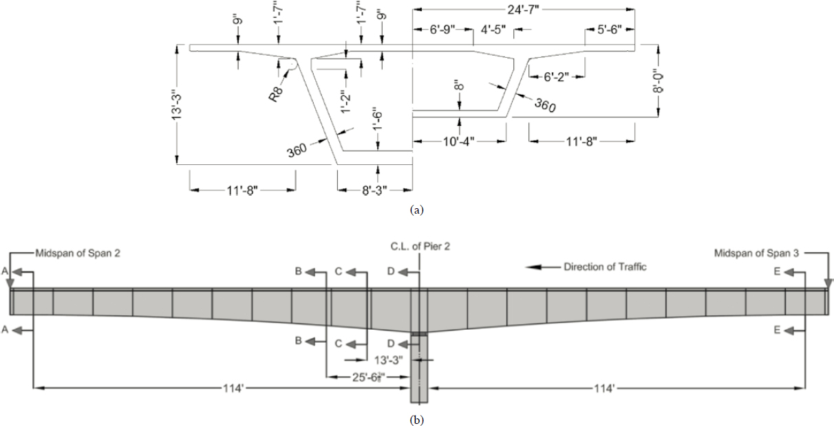
Figure 6-54. (a) Cross-sectional dimensions for the segmental bridge constructed with balanced cantilever method; and (b) illustration of sections (Sections A and C) that are considered for the validation study.

Figure 6-55. Instrumentation for (a) Section A (near midspan) and (b) Section C (near pier) (the blue and red colors stand for longitudinal and transverse strain, respectively).
was modeled using standard quadratic shell elements (S8R) by extruding the mid-surface of the cross section as shown in Figure 6-57(a). Since the goal of the comparative analysis was to compare the live load effects predicted using various methods, only the concrete cross section was modeled (i.e., the tendons were not included in the model). The bridge has 10 spans. However, since the areas of the bridge affected by the position of trucks used in the live load tests is limited, only two of the spans were modeled in the longitudinal direction as shown in Figure 6-57(b).
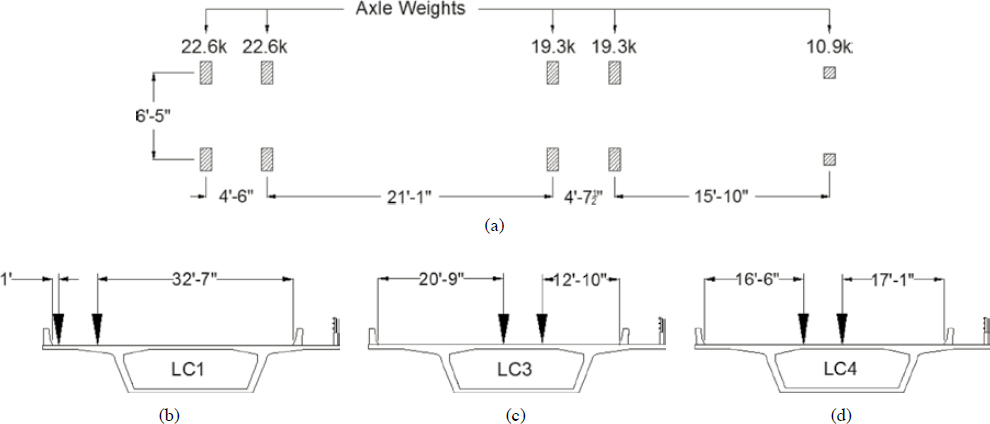
Figure 6-56. (a) FDOT truck dimensions and axle weights and (b–d) load combinations used for the validation of transverse analysis.

The following assumptions were made when creating the 3D model:
- A second order polynomial function was used to create the non-prismatic cross section.
- The thickness of the bottom flange varies along the span length. The cross sections between the midspan and pier were divided into six segments, and separate bottom flange thicknesses were assigned to each segment.
- Similarly, the thickness of the top flange varies in the transverse direction. Various finite elements were used in the transverse direction and each element was assigned an average thickness.
- Boundary conditions were modeled as roller-pin-roller.
- A 150-mm- (5.9-in.-) mesh size was used for the locations where the strain gauges were positioned (Sections A and C). For all other locations, a 1,000-mm- (39-in.-) mesh size was selected as shown in Figure 6-58.
- A linear elastic analysis was conducted.
- The truck wheel loads were applied as concentrated point loads.
6.4.7.5 Influence of Section Length to Width Ratio on Transverse Analysis
In the previous section, it was noted that while the bridge features 10 spans, only two spans were modeled because the inclusion of additional spans was not deemed necessary because live load effects extend only a certain distance in the longitudinal direction. It is natural to ask, what

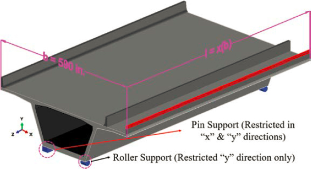
the minimum distance in the longitudinal direction needs to be and what are the appropriate boundary conditions. To address these questions, several models were created for the Seabreeze Bridge, each featuring a different bridge length in the longitudinal direction. The ratio of section length, l, and section width, b, varied from 1.0 to 3.0. The considered ratios were l/b = 1.0, l/b = 1.5, l/b = 2.0, and l/b = 3.0.
Additional models considered include one that featured the full span on which the live load was applied, and another that featured the simplified full span. The difference between the full span model and the simplified one is in terms of how the box cross section was modeled. In the full span model, the box cross section was modeled in its non-prismatic form. As noted previously, the shallowest section is 8 ft, and the deepest section is 13 ft 3 in. Similarly, the thickness of the bottom flange varies from 1 ft 6 in. to 8 in. The top flange also features a varying thickness. In the simplified model, the box cross section was modeled as a prismatic cross section featuring an average depth of 10 ft 7.5 in. The bottom flange was modeled with an average thickness of 13 in. The top flange was divided into three parts to simplify its modeling as illustrated in Figure 6-60. Each part was assigned the specified average thickness. In both cases that featured the full span, the ratio between bridge length to bridge width was l/b = 4.9.
The boundary conditions for each case were such that the box cross section was supported at each end underneath each web. At each end, pin supports were used under one web and roller supports were used under the other (see Figure 6-59). The live load case LC4 described earlier was used for this investigation. Shell finite elements featured quadrilinear elements with reduced integration (S4R). The mesh size for the top flange, webs, and bottom flange were 500 mm (19.7 in.), 750 mm (29.5 in.) and 1,000 mm (39.4 in.), respectively. As the section length was incrementally increased to investigate its effects, the position of the truck was always centered.
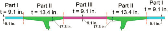
6.4.7.6 Results
6.4.7.6.1 Comparison of Results Obtained using Homberg Charts versus 3D FE Model
Table 6-16 shows the measured and computed live load induced normal strains in the transverse direction. The units for all reported values are in microstrain. The last two columns provide the ratio of computed over measured strains. In general, the computed strains obtained using the 3D shell FE model were more accurate than those obtained using the 2D frame model and Homberg charts, although in both cases, the V was large. This is attributed to the fact that, in some cases, the measured strains were rather small, which resulted in large computed to measured strain ratios. For example, for LC1 at Section A, the measured strains were reported as −1 µε and 1 µε, whereas computed strains based on the 3D FE model were −3 µε and 2 µε at the left and mid of the top slab, respectively. In this case, the ratios of measured to computed strains are 3.00 and 2.00, respectively, although the difference in magnitude between the measured and computed strains was negligible. Similar observations can also be made for other locations and truck positions. Therefore, the average computed to measured strain ratio and V given in Table 6-16 may be misleading in terms of prediction accuracy and consistency. Overall, the strains obtained using the 3D FE model were slightly lower than the measured strain.
Live load effect predictions based on the 2D frame model and Homberg charts were grossly conservative. The average computed to measured strain ratio was 4.46 and the V was 262%. Again, the large V is attributed to the small benchmark measured strain in some cases. Given the
Table 6-16. Measured and computed live load induced normal strains in the transverse direction.
| Location | Measured, εmea (µε) | 3D Shell FE Analysis εFE (µε) | 2D Frame Analysis with Homberg’s Charts, εHomb | Ratio | |
|---|---|---|---|---|---|
| LC1 - Section A | |||||
| Wing | -42 | -36 | -58 | 0.86 | 1.38 |
| Left Top S. | -1 | -3 | -49 | 3.00 | 49.00 |
| Mid Top S. | 1 | 2 | -7 | 2.00 | -7.00 |
| LC3 - Section A | |||||
| Wing | -4 | 0 | 0 | 0.00 | 0.00 |
| Left Top S. | -19 | -23 | -38 | 1.21 | 2.00 |
| Mid Top S. | 38 | 27 | 38 | 0.71 | 1.00 |
| LC4 - Section A | |||||
| Wing | -6 | -1 | 0 | 0.17 | 0.00 |
| Left Top S. | -19 | -15 | -40 | 0.79 | 2.11 |
| Mid Top S. | 53 | 44 | 50 | 0.83 | 0.94 |
| LC1 - Section C | |||||
| Wing | -19 | -36 | -58 | 1.89 | 3.05 |
| Left Top S. | -5 | -16 | -43 | 3.20 | 8.60 |
| Mid Top S. | -1 | -1 | -11 | 1.00 | 11.00 |
| LC3 - Section C | |||||
| Wing | -3 | -1 | 0 | 0.33 | 0.00 |
| Left Top S. | -14 | -13 | -36 | 0.93 | 2.57 |
| Mid Top S. | 27 | 26 | 41 | 0.96 | 1.52 |
| LC4 - Section C | |||||
| Wing | -6 | 0 | 0 | 0.00 | 0.00 |
| Left Top S. | -17 | -9 | -42 | 0.53 | 2.47 |
| Mid Top S. | 33 | 25 | 55 | 0.76 | 1.67 |
| Note: All strain values are given in terms of microstrain, µε. | Average | 1.07 | 4.46 | ||
| St. Dev. | 0.91 | 11.70 | |||
| V (%) | 86 | 262 | |||
gross overestimation of live load effects using the Homberg charts and the simplicity of creating a 3D FE model in the transverse direction for predicting live load effects, it is recommended that the creation of a 3D model be considered. The use of Homberg charts may be appropriate for a preliminary evaluation of the bridge in the transverse direction. If it is determined that the rating is controlled primarily by the longitudinal direction, then a 3D model may not be needed. However, if the rating of the bridge is controlled by transverse behavior, then the creation of a 3D model is warranted as an additional posting mitigation consideration tool.
In addition, for Florida, Corven Engineering (2004) states that while for legal and permit loads, the permissible tensile stress in a transversely post-tensioned slab is set at ksi regardless of the environment, for posting mitigation a value of up to ksi may be allowed provided that
- There is sufficient bonded reinforcement to carry the calculated tensile force in the concrete computed on the assumption of an uncracked section at a stress of 0.5fy, and
- It is verified by field inspection that there are no cracks in the bridge deck as a consequence of routine or historically heavy vehicular traffic.
Similarly, the inclusion of barriers is another approach that may be considered when evaluating the need for posting. The presence of barriers, which act compositely with the concrete segmental cross section, helps distribute the loads in the longitudinal direction, thus increasing the portion of the top slab that participates in providing resistance in the transverse direction when subject to live loads. This stiffening effect reduces peak transverse moments at the root of cantilever and increases load rating. Similarly, the presence of median barriers may provide the same benefits at other locations on the top slab (Corven Engineering 2004). When structurally composite barriers are included in the load rating analysis, transformed-section properties should include the difference in elastic moduli between the barrier and segment concrete. The presence of joints in the barrier should also be considered because at such joints the section properties reduce to those of the transformed concrete segment alone and stress concentrations may arise. Nevertheless, both longitudinal and local transverse load rating should benefit from reasonable consideration of barrier stiffness (Corven Engineering 2004).
Figure 6-61 shows the normal strain contours in the transverse direction in the top slab for the considered truck positions. The locations where the strain gauges were installed were preselected in FE model, and the normal strains in the transverse directions were obtained. The higher strain concentrations at the web supports at distances nearest to the applied live load may be clearly seen. The magnitude of the normal strain at the web supports diminishes as the distance from the applied live load increases. This effect is conceptually captured by the Homberg (1968) charts as well, although the FE model suggests a different distribution. This may stem from the fact that the FE model considers the top slab and web interaction in the transverse direction as well as the deformation of the superstructure in the longitudinal direction, thus resulting in a different live load distribution.
6.4.7.6.2 Influence of Finite Element Mesh Size
The sensitivity of normal strains in the transverse direction in the top slab to the size of the finite element mesh was investigated by considering five different mesh sizes ranging from 3.9 in. to 39.4 in. The variation of mesh size was conducted only for the region of interest described previously (i.e., between Section A and Section C). The mesh size at the other location was not changed. The results are provided in Table 6-17 and Figure 6-62. While Table 6-17 provides the results for all considered truck positions, Figure 6-62 illustrates the stability of normal strain magnitude only for LC4-Section A. The magnitude of normal strains in the transverse direction is virtually unaffected by mesh size, with variation in magnitude being approximately ±1 µε for some cases. Therefore, even a mesh size as large as 39.4 in. for the finite element type mentioned
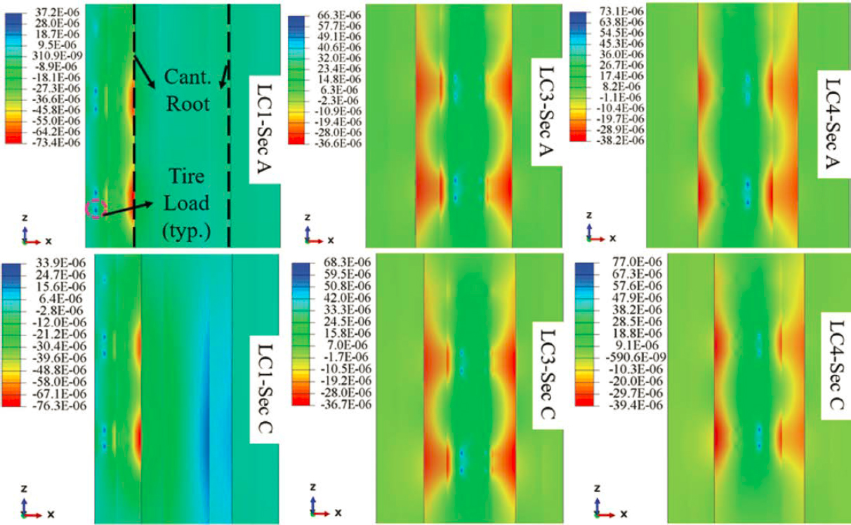
appears to provide consistent results compared with those obtained for smaller mesh sizes. The use of larger mesh sizes may be beneficial in cases when computational time is a concern.
6.4.7.6.3 Influence of Finite Element Type
The sensitivity of normal strains in the top slab in the transverse direction to the selected finite element type was investigated by considering five finite element types (Figure 6-63). This sensitivity analysis was conducted using a mesh size of 5.9 in. for the region of interest as discussed previously. The results are shown in Table 6-18 and Figure 6-64. While Table 6-18 shows the results of the sensitivity analysis for all truck positions considered, Figure 6-64 provides a graphic illustration of the normal strain magnitude stability for truck position LC4-Section A. The average ratios of computed to measured normal strains in the transverse direction are generally consistent with only minor variations. Although the S8R is the most advanced element type from the ones considered, other element types, such as S4, S4R, and S3, provide slightly more accurate predictions from the perspective of the average ratio of computed to measured normal strain. However, the lowest V, which is still quite large for reasons discussed previously, is obtained when the S8R element is used. Overall, the changes in strains due to the selection of element types and orders are not significant (i.e., in the order of ± 2 µε). Therefore, it can be concluded that the use of simple finite elements, such as the S3—linear triangular element, does not introduce notable error in the analysis. In addition, analysis time is greatly reduced to a total of 2.5 minutes—a 37% reduction considering that the benchmark model featuring S8R elements takes around 4 minutes to run.
Table 6-17. Live load induced normal strains in the transverse direction obtained from FE analysis based on different mesh sizes.
| Location | Measured, εmea (µε) (a) | FE Analysis, εFE (µε), with Mesh Size: | Ratio | ||||||||
|---|---|---|---|---|---|---|---|---|---|---|---|
| 3.9 in. (100 mm) (b) | 5.9 in. (150 mm) (c) | 7.9 in. (200 mm) (d) | 19.7 in. (500 mm) (e) | 39.4 in. (1000 mm) (f) | b/a | c/a | d/a | e/a | f/a | ||
| LC1 - Section A | |||||||||||
| Wing | -42 | -36 | -36 | -36 | -35 | -35 | 0.86 | 0.86 | 0.86 | 0.83 | 0.83 |
| Left Top S. | -1 | -3 | -3 | -3 | -3 | -3 | 3.00 | 3.00 | 3.00 | 3.00 | 3.00 |
| Mid Top S. | 1 | 2 | 2 | 2 | 2 | 2 | 2.00 | 2.00 | 2.00 | 2.00 | 2.00 |
| LC3 - Section A | |||||||||||
| Wing | -4 | 0 | 0 | 0 | 0 | 0 | 0.00 | 0.00 | 0.00 | 0.00 | 0.00 |
| Left Top S. | -19 | -23 | -23 | -23 | -23 | -22 | 1.21 | 1.21 | 1.21 | 1.21 | 1.16 |
| Mid Top S. | 38 | 27 | 27 | 27 | 27 | 25 | 0.71 | 0.71 | 0.71 | 0.71 | 0.66 |
| LC4 - Section A | |||||||||||
| Wing | -6 | -1 | -1 | -1 | -1 | -1 | 0.17 | 0.17 | 0.17 | 0.17 | 0.17 |
| Left Top S. | -19 | -15 | -15 | -15 | -15 | -14 | 0.79 | 0.79 | 0.79 | 0.79 | 0.74 |
| Mid Top S. | 53 | 44 | 44 | 44 | 44 | 45 | 0.83 | 0.83 | 0.83 | 0.83 | 0.85 |
| LC1 - Section C | |||||||||||
| Wing | -19 | -36 | -36 | -36 | -36 | -36 | 1.89 | 1.89 | 1.89 | 1.89 | 1.89 |
| Left Top S. | -5 | -16 | -16 | -16 | -16 | -17 | 3.20 | 3.20 | 3.20 | 3.20 | 3.40 |
| Mid Top S. | -1 | -1 | -1 | -1 | -1 | -1 | 1.00 | 1.00 | 1.00 | 1.00 | 1.00 |
| LC3 - Section C | |||||||||||
| Wing | -3 | -1 | -1 | -1 | -1 | -1 | 0.33 | 0.33 | 0.33 | 0.33 | 0.33 |
| Left Top S. | -14 | -13 | -13 | -13 | -13 | -13 | 0.93 | 0.93 | 0.93 | 0.93 | 0.93 |
| Mid Top S. | 27 | 26 | 26 | 26 | 26 | 28 | 0.96 | 0.96 | 0.96 | 0.96 | 1.04 |
| LC4 - Section C | |||||||||||
| Wing | -6 | 0 | 0 | 0 | 0 | 0 | 0.00 | 0.00 | 0.00 | 0.00 | 0.00 |
| Left Top S. | -17 | -9 | -9 | -9 | -9 | -9 | 0.53 | 0.53 | 0.53 | 0.53 | 0.53 |
| Mid Top S. | 33 | 25 | 25 | 25 | 25 | 26 | 0.76 | 0.76 | 0.76 | 0.76 | 0.79 |
| Note: All strain values are given in terms of microstrain, µε. | Average | 1.07 | 1.07 | 1.07 | 1.06 | 1.07 | |||||
| St. Dev. | 0.91 | 0.91 | 0.91 | 0.91 | 0.94 | ||||||
| V (%) | 86 | 86 | 86 | 86 | 88 | ||||||


Table 6-18. Live load induced normal strains in the transverse direction obtained from FE analysis based on various element type and element order.
| Location | Measured, εmea (µε) (a) | FE Analysis, εFE (µε), with Element Type and Order: | Ratio | ||||||||
|---|---|---|---|---|---|---|---|---|---|---|---|
| Base-Quad-Quadratic (S8R) (b) | Quad-Linear w/out Red. Int. (S4) (c) | Quad-Linear w/Red. Int. (S4R) (d) | Triangular-Quadratic (STRI65) (e) | Triangular-Linear (S3) (f) | b/a | c/a | d/a | e/a | f/a | ||
| LC1 - Section A | |||||||||||
| Wing | -42 | -36 | -36 | -36 | -36 | -37 | 0.86 | 0.86 | 0.86 | 0.86 | 0.88 |
| Left Top S. | -1 | -3 | -3 | -3 | -3 | -3 | 3.00 | 3.00 | 3.00 | 3.00 | 3.00 |
| Mid Top S. | 1 | 2 | 2 | 2 | 2 | 2 | 2.00 | 2.00 | 2.00 | 2.00 | 2.00 |
| LC3 - Section A | |||||||||||
| Wing | -4 | 0 | 0 | 0 | 0 | 0 | 0.00 | 0.00 | 0.00 | 0.00 | 0.00 |
| Left Top S. | -19 | -23 | -23 | -23 | -23 | -23 | 1.21 | 1.21 | 1.21 | 1.21 | 1.21 |
| Mid Top S. | 38 | 27 | 27 | 27 | 27 | 27 | 0.71 | 0.71 | 0.71 | 0.71 | 0.71 |
| LC4 - Section A | |||||||||||
| Wing | -6 | -1 | -1 | -1 | -1 | -1 | 0.17 | 0.17 | 0.17 | 0.17 | 0.17 |
| Left Top S. | -19 | -15 | -15 | -15 | -15 | -14 | 0.79 | 0.79 | 0.79 | 0.79 | 0.74 |
| Mid Top S. | 53 | 44 | 43 | 43 | 45 | 43 | 0.81 | 0.81 | 0.81 | 0.85 | 0.81 |
| LC1 - Section C | |||||||||||
| Wing | -19 | -36 | -36 | -36 | -36 | -36 | 1.89 | 1.89 | 1.89 | 1.89 | 1.89 |
| Left Top S. | -5 | -16 | -16 | -16 | -17 | -16 | 3.20 | 3.20 | 3.20 | 3.40 | 3.20 |
| Mid Top S. | -1 | -1 | -1 | -1 | -1 | -1 | 1.00 | 1.00 | 1.00 | 1.00 | 1.00 |
| LC3 - Section C | |||||||||||
| Wing | -3 | -1 | 0 | 0 | -1 | 0 | 0.00 | 0.00 | 0.00 | 0.33 | 0.00 |
| Left Top S. | -14 | -13 | -13 | -13 | -13 | -13 | 0.93 | 0.93 | 0.93 | 0.93 | 0.93 |
| Mid Top S. | 27 | 26 | 26 | 26 | 26 | 26 | 0.96 | 0.96 | 0.96 | 0.96 | 0.96 |
| LC4 - Section C | |||||||||||
| Wing | -6 | 0 | 0 | 0 | 0 | 0 | 0.00 | 0.00 | 0.00 | 0.00 | 0.00 |
| Left Top S. | -17 | -9 | -9 | -9 | -9 | -9 | 0.53 | 0.53 | 0.53 | 0.53 | 0.53 |
| Mid Top S. | 33 | 25 | 25 | 25 | 25 | 25 | 0.76 | 0.76 | 0.76 | 0.76 | 0.76 |
| Note: All strain values are given in terms of microstrain, µε. | Average | 1.07 | 1.05 | 1.05 | 1.08 | 1.04 | |||||
| St. Dev. | 0.91 | 0.93 | 0.93 | 0.94 | 0.93 | ||||||
| V (%) | 86 | 89 | 89 | 87 | 89 | ||||||
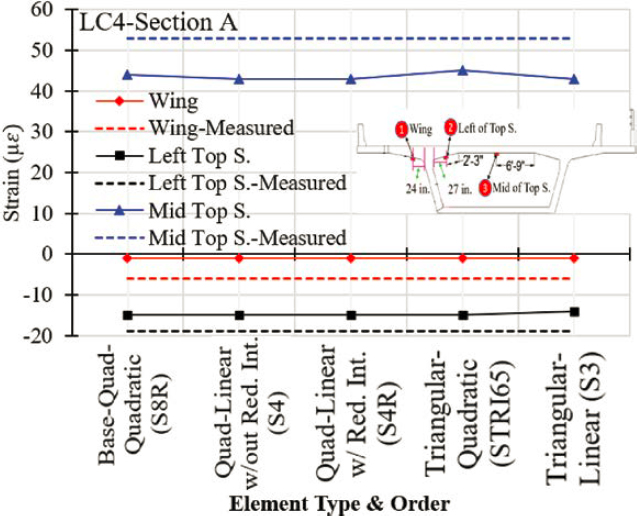
6.4.7.6.4 Influence of Section Length to Width Ratio
Table 6-19 provides a comparison of transverse normal strain at Section A for LC4. The comparison is provided between computed and measured strains. However, the results are also evaluated for how the predicted strains compared with one another. For example, the computed transverse normal strains between the actual full span model which featured non-prismatic cross sections and the simplified full span model are almost identical. Therefore, the averaging approach presented earlier for modeling the cross section depth, thickness of bottom flange, and thickness of top flange is a reasonable approximation. This saves considerable modeling time as it allows the analyst to model the bridge using a prismatic cross section and prismatic segments for the top and bottom flange.
Once it is established that the simplified full span model may be used to conduct transverse analysis, the results are evaluated for whether further simplifications in modeling may be pursued, specifically in terms of the length of the span to be modeled.
Table 6-19. Analysis results for the transverse analysis for LC4 at Section A using different box lengths (comparison with measured strains).
| Location | Strain (µε) – LC4 Section A | Ratio | |||||||||||
|---|---|---|---|---|---|---|---|---|---|---|---|---|---|
| Mea., εmea (a) | Actual Full Span1 (l = 4.9b) (b) | Simplified Full Span2 (l = 4.9b) (c) | l = b (d) | l = 1.5b (e) | l = 2.0b (f) | l = 3.0b (g) | b/a | c/a | d/a | e/a | f/a | g/a | |
| Wing | -6 | -5 | -4 | -2 | -2 | -3 | -3 | 0.8 | 0.7 | 0.3 | 0.3 | 0.5 | 0.5 |
| Left Top Slab | -19 | -15 | -15 | -20 | -15 | -15 | -15 | 0.8 | 0.8 | 1.1 | 0.8 | 0.8 | 0.8 |
| Mid Top Slab | 53 | 44 | 48 | 68 | 53 | 49 | 49 | 0.8 | 0.9 | 1.3 | 1.0 | 0.9 | 0.9 |
| 1The analysis was initially conducted without any additional simplifications that were mentioned previously except for reducing the number of spans to one. 2Analysis was conducted for the entire span (single span only) using the simplifications mentioned in this study in addition to the actual model that was presented before. | Avg. | 0.8 | 0.8 | 0.9 | 0.7 | 0.7 | 0.7 | ||||||
| V (%) | 3.0 | 15.2 | 55.7 | 48.2 | 29.4 | 29.4 | |||||||
Table 6-20. Analysis results for the transverse analysis for LC4 at Section A using different box lengths (comparison with strains obtained from simplified model).
| Location | Strain (µε) –LC4 Section A | Ratio | |||||||
|---|---|---|---|---|---|---|---|---|---|
| Simplified Full Span (l = 4.9b) (a) | l = b (b) | l = 1.5b (c) | l = 2.0b (d) | l = 3.0b (e) | b/a | c/a | d/a | e/a | |
| Wing | -4 | -2 | -2 | -3 | -3 | 0.5 | 0.5 | 0.8 | 0.8 |
| Left Top Slab | -15 | -20 | -15 | -15 | -15 | 1.3 | 1.0 | 1.0 | 1.0 |
| Mid Top Slab | 48 | 68 | 53 | 49 | 49 | 1.4 | 1.1 | 1.0 | 1.0 |
| Avg. | 1.1 | 0.9 | 0.9 | 0.9 | |||||
| V (%) | 46.8 | 37.2 | 16.3 | 16.3 | |||||
Table 6-20 provides a comparison of computed transverse normal strains using the full span simplified model and various models that featured different length of cross-section width ratios. An examination of the results suggests that models that featured cross-section lengths that are at least l = 2b provide a close enough approximation of the transverse normal strains compared with the full span model. As such, models with longer span lengths need not be pursued. This conclusion is illustrated further in Figure 6-65 and Table 6-21. In Table 6-21, it becomes clear that in the model where l = 2b, the green areas representing zero transverse normal strain, surround the nonzero transverse strain fields thus suggesting that a longer section is not necessary. The same cannot be said for models that feature l = b and l = 1.5b span lengths because the nonzero strain fields are interrupted by the ends of a segment. As a general rule, if the length of the span is l ≥ 2b and if the length of the span is such that it extends a distance of b/2 past the first and last line of wheels on each side, transverse normal strains should be predicted with sufficient accuracy for the purpose of transverse analysis if the guidance provided in this report regarding finite element type, finite element mesh, and boundary conditions is followed.
6.4.8 Conclusions for Comparative Analysis
The following conclusions were drawn from the comparative analysis.
- The selection of various creep and shrinkage models resulted in up to a 9% change in rating factors for the bridge constructed with the span-by-span method when the rating time was 10,000 days after the completion of construction and opening of the bridge to traffic. The limit state that was influenced the most was service flexure, followed by principal web tension. For the bridge constructed with the balanced cantilever method, the change in the
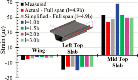
Table 6-21. Transverse analysis for LC4 at Section A using different box lengths.
| Case | Transverse Strains |
|---|---|
 |  |
 |  |
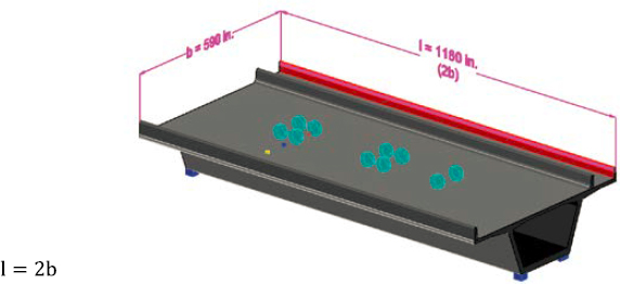 | 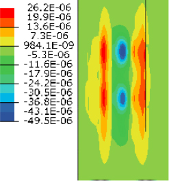 |
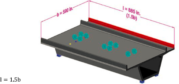 | 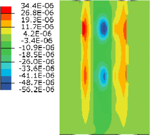 |
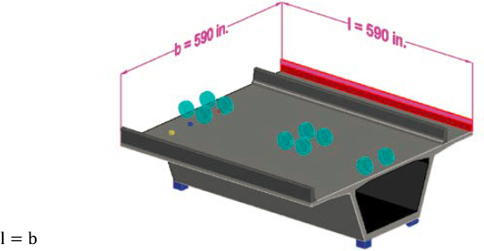 | 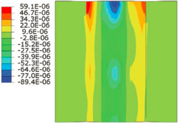 |
- Temperature gradient is a significant contributor to tensile stresses at service. Its relative contribution was quantified with respect to other load cases. It is recommended that temperature gradient effects be based on the provisions of AASHTO LRFD (2020a) using appropriate load combinations. Local reliable data may be used as an alternative to AASHTO LRFD (2020a) specified gradients to benefit load rating. The extent of tensile stresses along the depth of the cross section depends largely on the shape of the member. The prediction of temperature gradient-induced stresses should be based on strain compatibility analysis that considers the formation of free and restrained stresses at the cross-sectional level as well as stresses created due to restraining forces.
A 30% increase in the compressive strength overstrength factor resulted in up to a 45% increase in the controlling rating factor for some cases. The primary mechanism of this influence was through the allowable tensile stress, which is expressed as a function of f ′c. Therefore, the use of expected or actual material properties rather than specified material properties has the potential to result in a notable increase in rating factors. It is recommended that actual compressive strength based on test data be used to compute allowable stresses for load rating. The following approaches may be used to account for differences between specified strength and actual strength:
- Use the specified fc′ and adjust for increase with age. The following models may be used:
- ACI 209R-92
- CEB-FIP 1990
- fib 2010
- Where mechanical properties have been established by testing, follow guidance provided in AASHTO MBE (2018) Section 6A.5.2.1:
- The nominal value for strength is typically taken as the mean of the test values minus 1.65 standard deviation to provide a 95% confidence limit.
- Average test values should not be used for evaluation.
- Guidance on material sampling for bridge evaluation is provided in Article 5.3 of AASHTO MBE (2018).
- Use the specified fc′ and adjust for increase with age. The following models may be used:
- The selection of the time-dependent concrete compressive strength development model did not have a significant influence on load rating. The variation of the modulus of elasticity of concrete with time is expressed as a function of the variation of compressive strength with time. The considered models were ACI 209R-92 (ACI 1992) and CEB-FIP (1990). The change in rating factors was less than 3% when CEB-FIP (1990) model was considered as the benchmark model. Either ACI 209R-92 (ACI 1992) or CEB-FIP (1990) may be used for load rating.
- The selection of the allowable stress value had a strong impact on rating factors for the principal tensile stress limit state. The calculation of the allowable principal tensile stress may be computed using actual compressive strength or expected compressive strength when
load rating factors was up to 20% for service flexure. For strength limit states, the selection of various creep and shrinkage models resulted in changes of less than 3% in the rating factors. Some creep and shrinkage models resulted in higher relative creep and lower relative shrinkage. This resulted in a canceling effect in terms of their influence on prestress losses, and it dampened the influence of model selection on load rating. The time when the load rating is conducted will influence the impact that the creep and shrinkage models have on load rating. This influence is because the time when the load rating is conducted will determine the amount of creep and shrinkage that has taken place. This amount depends on the selected model. Therefore, the difference in predictions between the models may be higher or lower compared with the considered 10,000 day benchmark and will depend on the actual bridge age when the rating is conducted. It is recommended that any of the creep and shrinkage models currently allowed by AASHTO LRFD (2020a) for design be allowed to be used for load rating to maintain the same level of flexibility that is allowed in design.
- Three load rating times, 5,000 days, 10,000 days, 15,000 days after the completion of construction and the opening of the bridge to traffic, were considered. The difference in rating factors was less than 6% when CEB-FIP 1990 was selected as the model to predict creep and shrinkage behavior. There was a consistent trend toward lower rating factors as the bridge age increased. This was because for the rating times considered, the prestress losses increased as the bridge aged and thus the rating factors decreased. While the majority of the creep had taken place for the selected times and creep model, shrinkage had not yet reached its ultimate value. This affects secondary tensile stresses created due to shrinkage as well as prestress losses. The limit state that was affected the most by the rating time was service flexure, followed by principal web tension. The ultimate limit states were barely affected by the rating time for the cases considered in this study. Since the general tendency is toward smaller rating factors as the bridge gets older, rating the bridge at initial and final ages when load rating for legal and permit loads appears sufficient.
- The impact of the use of transformed versus gross-section properties on load rating was investigated. The difference in rating factors was up to 6.5% for service flexure. The limit state that was affected the most was service flexure, followed by principal web tension. The impact of using gross- versus transformed-section properties on ultimate strength limit states was limited to a 1.5% change in rating factors. Stresses caused by load components that are applied after the post-tensioning operations are complete may be based on transformed-section properties to benefit load rating.
- The selection of condition factors has a strong influence on load rating. A 15% decrease in the condition factor causes up to a 42% decrease in the rating factors. Similarly, a 10% increase in the condition factors causes up to a 17% increase in the rating factors. The use of condition factors should not be used as a replacement for a thorough inspection. Thorough inspections should be conducted and cross-sectional reductions or other types of deterioration in the prestressing strands or concrete cross section should be noted and taken into account in load rating calculations. In addition, appropriate condition factors should be used at the ultimate limit state to account for the increased uncertainty in the behavior of a deteriorated bridge compared with that of an undeteriorated bridge.
- The influence of multiple trucks on three two-lane concrete segmental bridges was investigated. The rating in the longitudinal direction was controlled by the two-lane loaded configuration over the one-lane loaded configuration. The rating in the transverse direction was controlled by the one-lane loaded configuration with the root of the cantilever generally being the controlling location.
- The influence of lane configuration was investigated by considering a concrete segmental bridge that could be configured as two (striped lanes) or three lanes (design lanes). The influence of lane configuration in the longitudinal direction was a consistent 22% change in the rating factors. For the transverse direction, the use of two lanes (striped lanes) versus three lanes (design lanes) did not result in any consistent benefit to load rating. For ratings in the longitudinal and transverse directions, the notional live load is placed to create worst-case effects in compliance with the guidance provided in AASHTO MBE (2018).
- The influence of the analytical technique on load rating in the transverse direction was considered. Measured live load induced strains reported for the Seabreeze Bridge were compared with those predicted using the Homberg charts combined with a 2D frame model, as well as those predicted by a 3D shell FE model. Predictions based on Homberg charts were overly
test data are not available. The principal tensile stress check was conducted at every joint along the span of the beam and at the centroidal axis along the cross section of the beam. As a minimum, the principal tensile stress check should be conducted as described. If there is reason to believe that the critical principal tensile stress may exist at locations other than the centroidal axis, due to the presence of ducts or other effects, then the principal tensile stress should be conducted at additional elevations along the depth of the cross section.
- When 3D FE modeling is used for conducting transverse analysis, non-prismatic cross sections may be approximated as prismatic cross sections using average section dimensions. In addition, the length of the bridge that needs to be modeled in the longitudinal direction needs to be such that l ≥ 2b where l is the length of the span and b is the width of the cross section. Boundary conditions may consist of pin and roller supports at each end of the section underneath each web.
- The influence of erection speed had minimal effect on load rating factors for the two considered scenarios for the bridge constructed with the span-by-span method.
- The inclusion of the Resal effect for the bridge constructed with the balanced cantilever method resulted in up to a 12% change in load rating factors. The inclusion of the Resal effect may be used to benefit rating as an additional posting mitigation consideration tool. While the inclusion of the Resal effect may be used to benefit rating as an additional posting mitigation consideration tool, negative Resal effects must be included. This scenario is present in constant depth boxes with variable thickness in the bottom flange.
conservative. The results from the shell FE model were more accurate on average. Normal strain magnitude was found to be insensitive to mesh size (for the mesh sizes considered) and to the finite element type. The use of 3D FE models is recommended as an additional posting mitigation consideration tool for cases when the load rating of the bridge is controlled by the transverse direction.
6.5 Reliability Assessment of Service and Strength Limit States
6.5.1 Selection of Representative Structures
Due to data availability, six bridges were ultimately selected for calibration as listed in Table 6-22. The first three examples of idealized bridges from Chapter 5 were also used in the reliability analysis. The characteristics of all bridge structures used in the reliability analysis (some of them are parts of whole bridge structures) are shown in Table 6-27.
6.5.2 Formulation of the Limit State Functions
Structures and structural components are either considered safe or in a state of failure. A limit state is a state of the structure on the borderline between safety and failure. Formulation of a limit state requires a definition of what is acceptable and unacceptable. A mathematical expression
Table 6-22. Representative structures.
| State | Bridge ID | Year built | Material | Max Span Length (ft) | Total Span Length (ft) | Number of Spans in Main Unit | Deck Width (ft) | Number of Lanes | Erection Type | ADTT per Lane | Rating Method | Superstructure Condition |
|---|---|---|---|---|---|---|---|---|---|---|---|---|
| Florida | 890150 | 2006 | P/C Cont. | 152 | 4,661 | 31 | 61 | 2 | Span-by-Span | 455 | LRFR | Good |
| 150189 | 1986 | P/C Cont. | 1,200 | 21,877 | 11 | 95 | 4 | Span-by-Span | 1078 | LRFR | Good | |
| 580174 | 1999 | P/C Cont. | 225 | 18,425 | 131 | 43 | 2 | Span-by-Span | 595 | LRFR | Fair | |
| North Carolina | 5140182P | 1983 | P/C Cont. | 508 | 1,249 | 8 | 45 | 2 | Progressive Cantilever | 718 | LRFR | Good |
| Tennessee | 5460214P | 2013 | P/C Cont. | 180 | 790 | 5 | 38 | 2 | Balanced Cantilever | 340 | AS | Good |
| Colorado | F-07-AL | 1986 | P/C Cont. | 132 | 613 | 5 | 38 | 2 | Span-by-Span | 553 | LF | Good |
that describes a limit state is called a limit state function. There are numerous types of limit states in AASHTO LRFD and LRFR, including strength limit states, service limit states, fatigue limit states, and extreme event limit states. The simplest limit state function is as follows:
| (6-26) |
Where R is resistance (load-carrying capacity) and Q is load effect. As long as g ≥ 0, the structure is safe. The probability of failure, Pf, is equal to the probability that g < 0.
As discussed previously, various segmental bridge limit states must be considered. These include the following:
- Flexural tensile stress (service)
- Flexural compressive stress (service)
- Principal tensile stress (service)
- Flexure (strength)
- Shear (strength)
Although each limit state was investigated and considered, a determination was made about which limit states to include in the calibration. Two primary criteria were used to assess suitability for inclusion: (1) is there a feasible analytical model and are statistical data available to allow formulation and calibration of the limit state, and (2) is the limit state useful for rating. A key issue that was addressed is the development of the criteria for acceptability (i.e., what specific limit would indicate a rating factor equal to 1.0).
For some limit states, the formulation of what is acceptable and what is unacceptable involves a subjective judgment. In such cases, the Delphi method can be applied to leverage expert opinion, as it was applied in SHRP2 R19B (Modjeski and Masters, Inc. et al. 2015).
For each limit state, a mathematical formulation was developed with corresponding parameters representing load and resistance. Such formulations were based on currently acceptable analytical models to determine resistance and load effect. In some cases, load effects may be determined or validated by appropriate numerical modeling approaches as needed. Appropriately simplified approaches were developed for use during the calibration process such that it remained viable.
6.5.3 Development of Statistical Models for Load
The truckloads are known to cause effects on the serviceability and deterioration of bridges (Yang, Lou, and Nassif 2024; Yang, Wang, and Nassif 2024). In addition, the live load effects for segmental bridges were anticipated to differ from that of slab-on-girder bridges. Since the load will be distributed across the entire bridge cross section, a heavy vehicle used in operating rating or permit rating typically produces less load increment in a segmental bridge than in a girder bridge when compared with inventory rating, and segmental bridges (particularly long spans) exhibit much higher dead-to-live load ratios than girder bridges.
However, the switch from the HS 20-44 truck to the HL-93 truck plus lane or tandem plus lane load posed a challenge for the load rating of concrete segmental bridges that were designed using AASHTO’s Standard Specifications for Highway Bridges. Some concrete segmental bridges do not achieve target ratings as a result of this alteration, which increases the load requirement. Corven Engineering (2004) suggests using striped lanes rather than design lanes for calculating rating factors to account for decreasing reliability under operating conditions.
Also, AASHTO MBE Section 6A.5.11.4 suggests that “for operating rating of the design load at the service limit state, the number of live load lanes may be taken as the number of striped lanes. However, loads shall be positioned so as to create maximum effects, for example, on shoulders if necessary.” The reason of considering striped lanes is “to calibrate the service limit states and
distinguish the operating rating from the inventory rating.” It is also stated that “while the use of number of striped lanes results in lower reliability for ratings at the service limit states, the resultant increment in βT is unknown.”
It was concluded in the current AASHTO MBE that the use of number of striped lanes is appropriate for operating ratings based on a brief study of existing bridges. However, in terms of bridge reliability, more rigorous calibration is needed to justify such conclusion. The research team reexamined the multiple presence factor, targeting segmental bridges, which are typically wider and have longer span lengths than the slab-on-girder bridges.
6.5.3.1 WIM Site Selection
The live load statistical model depends greatly on the actual traffic scenarios. The WIM techniques that capture the traffic data were used to develop the load model in this study.
In this project, 6-year data (from 2014 to 2019) from 24 WIM sites in California were deployed in the live load model development. Among the 24 WIM sites, nine sites are bidirectional, and the others are one-directional. The bidirectional data did not necessarily have similar statistics (e.g., ADTT, truck weight), and therefore, the bidirectional data were processed separately per direction, for a total of 33 WIM sites.
6.5.3.2 WIM Data Quality Assurance
The WIM data includes several measurement errors due to various reasons that need to be recognized in the data review process. There are various reasons for questioning the data, such as very low gross vehicle weight (GVW), unrealistic configuration, and unreasonably fast speed. Therefore, the data were first filtered to eliminate the erroneous vehicle records using the criteria developed under NCHRP Project 12-83 Filtering Criteria 1, as shown in Figure 6-66 (Wassef et al. 2014).
After the WIM data were filtered as recommended under NCHRP Project 12-83, additional quality assurance was performed to avoid accounting for the WIM data that were out of calibration. The WIM data validating methodology developed by Southgate (2000) was applied, in which the front axle weights (FAW) of FHWA Class 9 truck (3S2, semi-tractor trailer) are regressed to first axle spacing. Southgate used these Class-9-3S2-type trucks not only because they are common commercial trucks but also because they have a stable relationship between the FAW and the steering axle spacing. He established a logarithmic relation between those two variables and used this relation to adjust WIM data. This technique uses the relationship between the first axle spacing (S12) and the ratio between steering axle weight and first axle spacing (A1/S12). The upper bound is formed by the 12-kip legal weight limit, and the lower bound is sourced from the truck manufacturer’s minimum specifications. If the regression curve of all Class 9 falls within the upper and the lower boundary and is close to the reference equation, then the quality of WIM data is acceptable.
The Southgate algorithm has been applied to all the WIM sites, and the data quality check was performed for annual data rather than all-year data together. The typical Southgate plots for a set of good quality data and a set of poor quality data are shown in Figure 6-67.
Last, to do live load analysis other than the permit load and fatigue load, the permit or heavy illegal overloaded vehicles should be excluded from the analysis (Wassef et al. 2014). The filters to identify the permit and heavy illegal overweight trucks are as follows:
- Total number of axles is less than three and GVW is more than 50 kips (Wassef et al. 2014).
- Steering axle weight is more than 25 kips (Wassef et al. 2014; Davis 2007).
- Individual axle weight is more than 45 kips (Wassef et al. 2014).
- There are seven or more axles (Sivakumar et al. 2011).
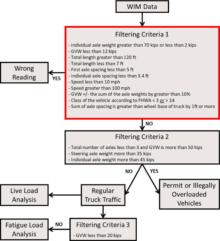
Figure 6-66. WIM data filters.

After all the filtering and quality assurance, the ADTT, excluding the permit and illegal overweight truck, is computed as tabulated in Table 6-23. In the same table, the number of days per year is also summarized. The quality of the annual data is represented by different colors. Green represents good data quality, which conforms well to the Southgate algorithm; red color represents poor data quality. The annual data that have poor quality were not used in this study.
6.5.3.3 Multiple Presence Factor for Longitudinal Direction
The study on the live load model focused on the MPF. AASHTO MBE prescribes the MPF in Table 3.6.1.1.2-1, as shown in Figure 6-68. When the current MPF was calibrated (Nowak 1999), there was a lack of an accurate WIM system, and therefore, assumptions have been made to simulate the two-lane load effects:
- Every 15th truck is on the bridge simultaneously with another truck (side-by-side).
- For each simultaneous occurrence, every 10th time, the trucks are partially correlated.
- For each simultaneous occurrence, every 30th time, the trucks are fully correlated with regard to weight.
The results of simulations based on these assumptions show the case where two fully correlated side-by-side trucks govern. Each truck in this simultaneous occurrence case is equal to the maximum 2-month truck and the load effects were obtained for a series of slab-on-girder bridges with a span length from 10 ft to 200 ft.
Table 6-23. WIM site information summary.
| Site No. | Direction | ADTT (Regular Truck Traffic) | Number of Days | |||||
|---|---|---|---|---|---|---|---|---|
| 2014 | 2015 | 2016 | 2017 | 2018 | 2019 | |||
| 001 | 1 | 4,193 | 326 | 167 | 338 | 330 | 114 | 36 |
| 2 | 3,811 | 326 | 167 | 338 | 330 | 113 | 36 | |
| 002 | 1 | 2,666 | 365 | 365 | 365 | 365 | 290 | 148 |
| 2 | 2,745 | 365 | 365 | 365 | 365 | 290 | 148 | |
| 003 | 1 | 3,280 | 365 | 365 | 364 | 365 | 285 | 102 |
| 004 | 1 | 3,106 | 365 | 335 | 366 | 365 | 289 | 148 |
| 027 | 1 | 3,095 | 360 | 252 | N.A. | N.A. | N.A. | N.A. |
| 2 | 3,208 | 360 | 253 | N.A. | N.A. | N.A. | N.A. | |
| 030 | 1 | 2,483 | 362 | 365 | 366 | 365 | 135 | N.A. |
| 2 | 2,536 | 362 | 365 | 366 | 365 | 135 | N.A. | |
| 037 | 1 | 2,991 | 365 | 365 | 366 | 320 | 96 | 4 |
| 038 | 1 | 2,626 | 365 | 350 | 351 | 305 | 290 | 141 |
| 041 | 1 | 3,299 | 122 | 365 | 366 | 365 | 290 | 152 |
| 042 | 1 | 3,548 | 122 | 365 | 366 | 365 | 290 | 152 |
| 057 | 1 | 3,191 | 355 | 365 | 366 | 363 | 290 | 152 |
| 058 | 1 | 3,378 | 365 | 365 | 366 | 363 | 290 | 152 |
| 059 | 1 | 11,814 | 356 | 365 | 365 | 365 | 259 | N.A. |
| 060 | 1 | 11,282 | 344 | 362 | 366 | 281 | N.A. | 152 |
| 065 | 1 | 1,000 | N.A. | N.A. | N.A. | 31 | N.A. | N.A. |
| 2 | 1,199 | N.A. | N.A. | N.A. | 31 | N.A. | N.A. | |
| 066 | 1 | 3,144 | 365 | 361 | 366 | 219 | N.A. | 141 |
| 2 | 3,277 | 365 | 361 | 366 | 219 | N.A. | 141 | |
| 067 | 1 | 2,454 | 365 | 347 | 366 | 365 | 290 | 116 |
| 2 | 2,845 | 365 | 347 | 366 | 365 | 290 | 116 | |
| 069 | 1 | 5,680 | 365 | 365 | 364 | 365 | 33 | N.A. |
| 070 | 1 | 5,176 | 365 | 365 | 366 | 365 | 33 | N.A. |
| 073 | 1 | 7,869 | 341 | 365 | 364 | 329 | 290 | 152 |
| 077 | 1 | 8,346 | 365 | 238 | 332 | 365 | 245 | 152 |
| 078 | 1 | 7,403 | 349 | 174 | 83 | 365 | 245 | 152 |
| 105 | 1 | 3,658 | N.A. | N.A. | N.A. | N.A. | N.A. | 102 |
| 2 | 3,881 | N.A. | N.A. | N.A. | N.A. | N.A. | 102 | |
| 108 | 1 | 3,092 | 314 | 349 | 366 | 365 | 131 | 152 |
| 2 | 3,052 | 314 | 349 | 366 | 365 | 131 | 152 | |
Note: N.A. = not available.
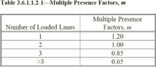
Figure 6-68. AASHTO MBE multiple presence factors.
With the advanced WIM technologies that are now available, the research team used the actual traffic data to investigate the multiple presence scenarios. To capture the relative position of each truck, the WIM data must have a time stamp displaying at least hundreds of a second. The selected WIM sites from Caltrans all have such time stamps.
The MPFs were developed based on two load indicators: truck weights and load effects caused by truck. The first load indicator, consistent with NCHRP Report 368, is based on the weight of the trucks that are traveling side-by-side (Nowak 1999). The second load indicator, as a validation of and an improvement to the first indicator, is based on the simultaneous load effects caused by the trucks that are on the bridge at the same time. Methodology previously developed by the research team was adopted to accurately capture the total load effects caused by multiple presence (MP) events and followed by the calculation of MPF (Lou et al. 2023; Yang et al. 2022; Lou et al. 2021). According to the bridge parameter statistics summarized in Section 6.1, the segmental bridges have a variety of maximum single-span lengths, ranging from 120-ft or less to 600-ft or more. Therefore, a series of simply supported bridges with span lengths from 30 ft up to 400 ft was considered in the analysis of the live load model. The span lengths were 30 ft, 60 ft, 90 ft, 120 ft, 200 ft, 300 ft, and 400 ft. The positive moment of simply supported spans are computed to obtain the live load bias ratio. Using the current MBE one-lane MPF of 1.2 as a benchmark, the two-lane, three-lane, and four-lane MPF can be calculated by using the bias ratio. Figure 6-69 through Figure 6-71 show the MPF results from typical two-lane, three-lane, and four-lane WIM sites, respectively. The overall statistics of the MPF of all the processed WIM sites are depicted by the box plot shown in Figure 6-72. It is worth noting that due to the cross-lane headways and the low probability of the four-lane loadings, the four-lane MPF for a span length of less than 120 ft could not be calculated.


As a result, multiple presence factors (m-factors) for segmental bridges are recommended as shown in Table 6-24.
6.5.3.4 Findings
Based on the selected WIM sites in this project, the findings are as follows:
- The MPFs calculated from truck weight and truckload effects showed agreement.
- The MPF was observed to be a function of span length.
- The current AASHTO MBE provided conservative MPF for bridges with a span length of less than 400 ft.
6.5.3.5 Thermal Effects
Thermal effects are transient but, under certain conditions, can generate forces and stresses that need to be accounted for during load rating. Nonlinear thermal gradients cause stresses in both simple span and continuous bridges. Concrete segmental bridges are designed for the effects of half thermal gradient (0.5 p TG) combined with full design live loads at service limit state (Corven Engineering 2004).
Thermal gradient effects are not considered when verifying bridge design at the strength limit state. Inventory ratings are conducted with the same level of reliability as new designs and should similarly include the effects of thermal gradients in accordance with AASHTO LRFD at the service limit state. In reality, the probability of the absolute maximum permissible live load
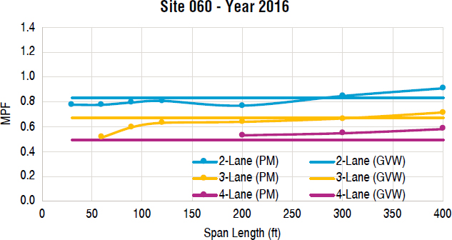

Table 6-24. Proposed m-factors.
| Number of loaded lanes | m-factor |
|---|---|
| 1 | 1.20 |
| 2 | 1.00 |
| 3 | 0.75 |
| 4 or more | 0.60 |
coinciding with the maximum effect of thermal gradient effect is low. Consequently, for inventory ratings, only 0.5 p TG is used along with the design live load at service (Corven Engineering 2004). For operating ratings, the effects of thermal gradient are not included at either the service or strength limit states as the influence of thermal gradient is not significant, and the consequences of exceeding the limit are not severe.
Typically, the longitudinal expansion and contraction of concrete bridges are managed by sliding or flexible bearings, which have minimal impact on the superstructure. However, forces induced by thermal expansion and contraction (TU) must be considered where the superstructures are rigidly connected to the substructures (Corven Engineering 2004). These forces should only be included at the service limit state for inventory ratings (with γTU = 1.0) because their inclusion at the strength limit state will likely not significantly impact the fundamental reliability of a structure and may result in extraneous tasks. For the operating rating, the influence of thermal expansion and contraction is deemed insignificant, and the consequences of exceeding the limit are not substantial.
6.5.4 Development of Statistical Models for Bridge Resistance
Resistance or load-carrying capacity can be considered as a function of three factors that represent uncertainty in (1) material properties (strength, modulus of elasticity), (2) dimensions (length, width, distance, area, a moment of inertia), and (3) the analytical model (the accuracy of the analytical model to represent actual behavior). To characterize these uncertainties as random variables, the statistical parameters commonly used for code calibration include bias factor (λ), coefficient of variation (V), and cumulative distribution function. It is important to include correlations between the parameters that determine the resistance. In this study, the statistical parameters of resistance were based on the available lab test data, field measurements, and simulations such as the Monte Carlo technique as documented in NCHRP Report 368 (Nowak 1999), Nowak and Collins (2013), and technical literature (Nowak and Szerszen 2003).
Load ratings of segmental bridges are frequently controlled by service limit states. Establishment of resistance in terms of element stress level can be done as under NCHRP Project 12-83. The team devoted attention to factors unique to segmental bridges, such as principal tensile stress in girder webs, and stress changes due to time-dependent and temperature-dependent material behavior. The development of analytical models for the resistance of segmental bridges and their components may require supporting testing or monitoring data that are not available. In such cases, the statistical parameters of interest can be determined using the Delphi method (i.e., expert opinion, as noted previously). Therefore, the project team sought the advice of practicing engineers designing and evaluating segmental bridges—relying on industry support partners such as the ASBI and Post-Tensioning Institute (PTI).
6.5.5 Development of the Reliability Analysis Procedure
Reliability indices were calculated for selected representative segmental bridges. For each representative bridge and each limit state, nominal load components and statistical parameters of a load were determined, with special attention to live load and dynamic load. However, the effects of uncertainty on load effects caused by internal forces, such as those from creep and shrinkage, changes in elastic modulus, and so forth, and the use of simplified analysis methods were also investigated. Then, a nominal value of resistance was determined, followed by statistical parameters of resistance. Using the statistical parameters of load and resistance, the reliability indices were calculated. The resulting reliability indices were grouped for different limit states and different rating vehicles, such as design load, AASHTO legal loads, single-unit trucks, and Fixing America’s Surface Transportation Act (FAST Act) EVs, and are presented in tables.
The reliability indices were calculated as follows:
| (6-27) |
where µR and µQ are mean values of load and resistance components, and σR and σQ are standard deviations of load and resistance.
6.5.6 Reliability Indices for Representative Bridges
Reliability analysis was performed to evaluate the structural condition of built segmental bridges. The results of the reliability analysis are presented in the following sections for the different limit states considered. From load rating factors in Appendix C of the Guideline, the most critical cases were taken as a basis to do the reliability procedure. In most cases, service limit states for tension at the bottom fiber of the segmental box section were the governing ones. In the following sections, results are shown for different construction types of segmental bridges.
6.5.6.1 Service Limit State—Flexure
Bridge information and material properties can be found in Appendix C of the Guideline.
For the Service III flexure limit state, the controlling rating factor was 1.05 at the 27th segment of the Example 1 bridge (midspan of second span, Figure 6-73). Controlling case was due to positive temperature gradient TG+.
The rating factor equation for this limit state is as follows:
| (6-28) |
where
| fall = | Allowable stress |
| fperm = | Stress due to permanent loads |
| fTG = | Stress due to temperature gradient |
| fTU = | Stress due to temperature uniform |
| γLL, γperm, γTG, γTU = | Load factors |
From the previous equation, the limit state function for the reliability analysis is derived as follows:
| (6-29) |
Using the values obtained from Midas Civil, nominal stresses were computed for all the load components to obtain mean values using the statistical parameters [bias factors and coefficients

of variation (V)] shown in Table 6-25. Statistical parameters for live load were taken from SHRP2 R19B (Modjeski and Masters, Inc. et al. 2015) for ADTT 5,000 and return period of 1 year.
Table 6-25. Statistical parameters for service limit states.
| Assumed Statistical Parameters | ||
| λ | V | |
| DC | 1.03 | 0.08 |
| DW | 1 | 0.15 |
| PS | 1.08 | 0.05 |
| LL | 1.13 | 0.09 |
Mean values were obtained by multiplying each nominal value by their respective bias factor. The standard deviation of the load component was obtained by multiplying the mean value with the respective coefficient of variation.
| (6-30) |
The nominal resistance was determined as the required prestressing stress to resist the total load.
In the reliability analysis, the mean total load was calculated using Turkstra’s Rule (Nowak and Collins 2013). The dominating parameters in Eq. (6-30) taking maximum values were µDC, µDW, and µLL, and the others were considered negligible. Therefore, the reliability index was calculated as follows:
| (6-31) |
No tension was allowed in the precompressed tensile zone for the Type A joints. Since allowable tension is zero, the equation becomes:
| (6-32) |
The critical locations for reliability analysis are over the supports for negative moment (top fibers) and midspan area for positive moment (bottom fibers). An example of the nominal stresses and statistical parameters is shown in Table 6-26 for segment 17 (area at the support, top fiber), which is the most critical for this bridge. Nominal PS stress was computed as follows:
| (6-33) |
Table 6-26. Example calculations for service limit state at top fiber segment 17.
| Nominal Stress, psi | Bias Factor, λ | Coefficient of Variation, V | Mean Value μ, psi | Standard Deviation σ, psi | |
| DC | 432 | 1.03 | 0.08 | 445 | 36 |
| DW | 145 | 1 | 0.15 | 145 | 22 |
| PS | -782 | 1.08 | 0.05 | -845 | -42 |
| LL | 205 | 1.13 | 0.09 | 232 | 21 |
| TU | 0 | ||||
| CR | -25 | ||||
| SH | 0 | ||||
| TG+ | -1,140 | ||||
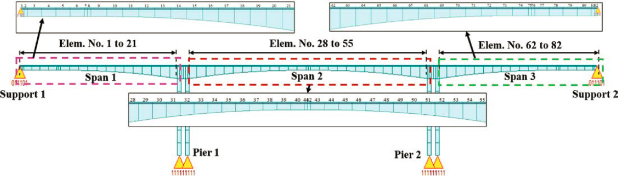
Using the values shown in Table 6-26, the reliability index for the 17th segment for Service III limit state is as follows:
| (6-34) |
The reliability indices were computed for the previously mentioned critical locations of the bridges, and the results are shown in Table 6-28.
The reliability assessment was also conducted for another example of a span-by-span bridge, structure No. F-07-AL in Colorado. The bridge has five spans; the external spans are 106 ft long, and the internal spans are 132 ft long. The depth of the cross section is 6 ft. The bridge is curved, and its cross section is inclined. The compressive strength of concrete is f′c = 5,500 psi, and the ultimate strength of the prestressing strands is fu = 270 ksi.
The elevation of the balanced cantilever bridge (Example 2) is shown in Figure 6-74.
The elevation of the incremental launching bridge (Example 3) is shown in Figure 6-75.
All bridge structures for which the reliability analysis was performed are shown in Table 6-27. Some of these are parts of whole bridge structures, such as an approach span unit in the Sunshine Skyway Bridge.
The minimum reliability indices along the length for the considered bridges are shown in Table 6-28. Dashes indicate the absence of live load data at the supports.
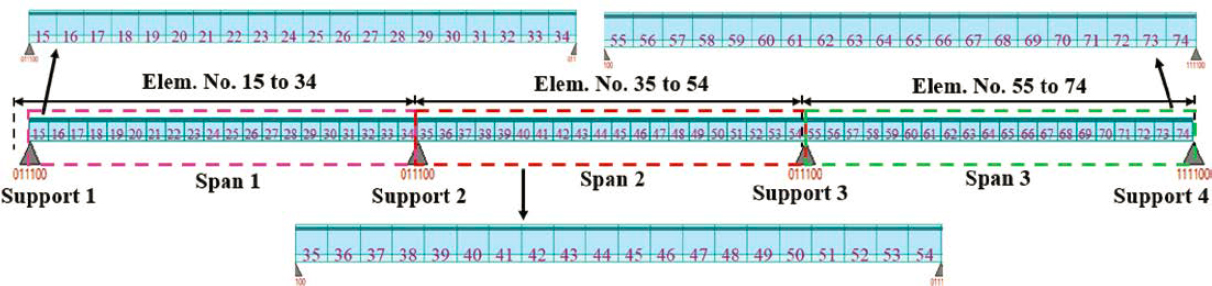
Table 6-27. Characteristics of the analyzed bridges.
| Name/Designation | State | Bridge ID | Year Built | Max. Span Length (ft) | No. of Spans | Deck Width (ft) | Construction/Erection Method |
|---|---|---|---|---|---|---|---|
| Foothills Bridge | Tennessee | 5460214P | 2013 | 180 | 5 | 36.8 | Balanced Cantilever |
| Ernest Lyons Bridge | Florida | 890150 | 2006 | 152 | 6 | 33 | Span-by-Span |
| Garcon Point Bridge | Florida | 580174 | 1999 | 225 | 8 | 43.1 | Balanced Cantilever/Span-by-Span |
| Sunshine Skyway Bridge | Florida | 150189 | 1986 | 135 | 6 | 42.75 | Span-by-Span |
| Linn Cove Viaduct | North Carolina | 5140182P | 1983 | 180 | 8 | 34.3 | Progressive Cantilever |
| N/A | Colorado | F-07-AL | 1986 | 132 | 5 | 38 | Span-by-Span |
| Example 1 | 148 | 3 | 27.9 | Span-by-Span | |||
| Example 2 | N/A | N/A | 426 | 3 | 42 | Balanced Cantilever | |
| Example 3 | 164 | 3 | 40.4 | Incremental Launching | |||
6.5.6.2 Service Limit State—Principal Web Tension
The approach, similar to that of the Service III flexure limit state, was performed for principal web tension. The statistical parameters for the allowable tension were assumed as follows: λ = 1.1, V = 0.12, and for the live load: λ = 1.13, V = 0.09. The prestressing stress was calculated using the available information in technical documentation, such as technical drawings and material specifications, for the considered bridges. For the Example 1 bridge, the lowest reliability was observed for segments 17 and 36. The lowest rating factor was for segment 17 for this limit state.
| (6-35) |
| (6-36) |
Table 6-28. Minimum reliability indices for considered bridges (Service III flexure limit state).
| Designation/Name | βmin in Top Fiber (at Supports) | βmin in Bottom Fiber (at Midspan) |
|---|---|---|
| Example 1 (Span-by-Span) | 0.37 | 0.77 |
| Example 2 (Balanced Cantilever) | 0.54 | 2.10 |
| Example 3 (Incremental Launching) | 0.45 | 0.71 |
| F-07-AL, Colorado (Span-by-Span) | 0.64 | 0.25 |
| Ernest Lyons Bridge (Span-by-Span) | 0.56 | 0.91 |
| Garcon Point Bridge - Main Unit (Balanced Cantilever) | 0.50 | 2.30 |
| Garcon Point Bridge - Typical Unit (Span-by-Span) | - | 1.43 |
| Sunshine Skyway Bridge (Span-by-Span) | - | 1.46 |
| Foothills Bridge (Balanced Cantilever) | 0.42 | 0.75 |
| Linn Cove Viaduct (Progressive Cantilever) | 0.50 | 6.42 |
Table 6-29. Minimum reliability indices for considered bridges (Service III principal web tension limit state).
| Designation | βmin |
|---|---|
| Example 1 (Span-by-Span) | 0.68 |
| Example 2 (Balanced Cantilever) | 0.72 |
| Example 3 (Incremental Launching) | 2.46 |
| F-07-AL, Colorado (Span-by-Span) | 1.08 |
The minimum reliability indices along the length for the Example 1, 2, and 3 bridges as well as for the F-07-AL, Colorado bridge, are shown in Table 6-29.
6.5.6.3 Strength Limit State—Flexure
A similar approach to the one used for service limit states was used for flexural strength. For strength limit states, the statistical parameters shown in Table 6-30 were used. PSsc are secondary forces from post-tensioning. A 7.5% V and 1.075 bias factor are assumed for capacity in this calculation.
Table 6-30. Statistical parameters for strength limit states.
| Assumed Statistical Parameters | ||
| λ | V | |
| DC | 1.03 | 0.08 |
| DW | 1 | 0.15 |
| PSsc | 1 | 0.05 |
| CR | 1 | 0.15 |
| SH | 1 | 0.15 |
| LL | 1.0 | 0.25 |
The prestressing stress was calculated using the available information in the technical documentation for the considered bridges. For the Example 1 bridge, the lowest reliability was observed for segments 21 and 40. The lowest rating factor was for segment 21 for this limit state.
| (6-37) |
| (6-38) |
The minimum reliability indices along the length for the Example 1, 2, and 3 bridges, as well as for the F-07-AL, Colorado bridge are shown in Table 6-31.
6.5.6.4 Strength Limit State—Shear in Web
The statistical parameters of λ = 1.18, V = 0.12 were assumed for shear capacity, and λ = 1.0, V = 0.2 were assumed for the live load in this calculation. No system factors are included in the analysis. The prestressing stress was calculated using the available information in the technical documentation for the considered bridges. For the Example 1 bridge, the lowest reliability was observed for segments 17 and 36. The lowest rating factor was for segment 17 for this limit state.
| (6-39) |
| (6-40) |
Table 6-31. Minimum reliability indices for considered bridges (longitudinal flexural strength limit state).
| Designation | βmin |
|---|---|
| Example 1 (Span-by-Span) | 5.25 |
| Example 2 (Balanced Cantilever) | 7.1 |
| Example 3 (Incremental Launching) | 7.73 |
| F-07-AL, Colorado (Span-by-Span) | 1.99 |
The minimum reliability indices along the length for the Example 1, 2, and 3 bridges, as well as for the F-07-AL, Colorado bridge are shown in Table 6-32. It should be noted that segmental bridges have two or more webs, which results in additional redundancy (parallel system from the reliability point of view).
6.5.7 Selection of the Target Reliability Index
The obtained reliability results served as a basis for the selection of the target reliability indices, βT.
The selection criteria of the target reliability index were as follows:
- Consequences of exceeding the limit state—they were the same for inventory and operating rating.
- Cost to reduce the probability of exceeding the limit state—a higher probability of exceeding the limit state was accepted for operating rating.
Therefore, target reliability index was lower for operating rating than for inventory rating.
The target reliability indices for different limit states were selected based on the current practice, as well as on the discussion with the industrial partners, as follows:
- Service Limit State—Flexure: inventory level—βT = 1.0, operating level—βT = 0.0.
- Service Limit State—Principal web tension: inventory level—βT = 1, operating level—βT = 0.
- Strength Limit State—Flexure: inventory level—βT =3.5, operating level—βT = 2.5.
- Strength Limit State—Shear in web: inventory level—βT =3.5, operating level—βT = 2.5.
6.5.8 Calculation of Load and Resistance Factors and Verification
The objective of this project was to develop a segmental bridge-specific guideline for rating of existing segmental bridges. Therefore, the focus was on the differences in rating of segmental and non-segmental bridges. There are several limit states considered, including strength and service limit states. In practice, Service III limit state governs, so it is important to focus on the comparison between the rating of segmental bridges and non-segmental bridges.
Rating can be considered at inventory or operating level. The difference between these two levels is attributed to the time. In Strength I limit state, the difference is represented by a live load factor that was 1.75 for inventory rating and 1.35 for operating rating. For Service III limit state, the current design live load is 0.8 of HL-93. This design live load is currently the same for operating and inventory rating. However, since 0.8 HL-93 serves the Service III rating well—for both inventory and operating rating—the live load factor can be further reduced for operating rating as proposed in this report.
Table 6-32. Minimum reliability indices for considered bridges (web shear strength limit state).
| Designation | βmin |
|---|---|
| Example 1 (Span-by-Span) | 2.16 |
| Example 2 (Balanced Cantilever) | 1.82 |
| Example 3 (Incremental Launching) | 2.18 |
| F-07-AL, Colorado (Span-by-Span) | 2.44 |
6.5.8.1 Calibration Procedures for Span-By-Span Construction of Segmental Bridges
This section describes the calibration procedures to obtain the load and resistance factors for span-by-span construction of segmental bridges. The team has previously derived the resistance prediction equation for a prestressed concrete girder subjected to flexural loading, as shown in Figure 6-76. Figure 6-76(c) shows the stress distribution diagrams at the decompression loading stage, either at the level of prestressing strands, or at the bottom fiber of the concrete girder. The corresponding decompression moment in addition to dead load can be represented as MDecp, and MDecb, respectively. Figure 6-76(d) shows the loading stage of maximum allowable tensile stress limit state while Figure 6-76(e) shows the cracked section when the stress of the bottom fiber of the concrete girder are higher than allowable tensile stress, and the crack is smaller than the maximum (allowable crack width limit state).
This study evaluates the decompression stage at the bottom fiber of the concrete girder. The decompression moment can be calculated as follows:
| (6-41) |
| (6-42) |
where
| Ac = | Area of concrete at the cross section considered. |
| Aps = | Area of prestressing steel in tension zone. |
| e = | Eccentricity of the prestressing force with respect to the centroid of the section. |
| Ec = | Modulus of elasticity of concrete. |
| Eps = | Modulus of elasticity of prestressing steel. |
| fse = | Effective stress in prestressing steel after losses. |
| I = | Moment of inertia of concrete section. |
| MD = | Dead load moment. |
| MDecb = | Decompression moment at the bottom of the girder. |
| Itransfer = | Moment of inertia of transferred section. |
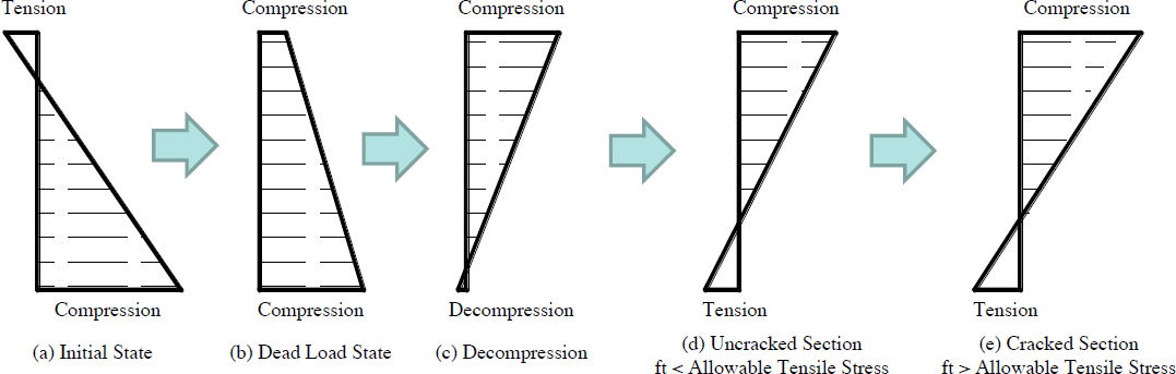
In NCHRP Project 12-83, four sets of design cases were developed for ASBI box girder bridges, including sections 1800-2, 2100-2, 2400-2. The designs are differentiated by different maximum tensile stress, including , , , . The span lengths range from 100 ft to 200 ft. Then reliability analysis was performed for those design cases under the live load of ADTT equals to 5,000 and return period of 1 year. Concrete compressive strength is 8,000 psi. The reliability indices for live load factors of 0.8 and 1.0 are shown in Figure 6-77. The average indices are 1.08 and 1.41 for live load factor of 0.8, and 1.0, respectively.
This study used the previous design example and focused on the reliability index for the Service III limit state at operating level. For the load rating of Service III limit state, the generalized load rating equation is shown as follows:
| (6-43) |
Then, the minimum required resistance, assuming the rating factor is satisfied, can be given as follows. This equation is used to determine the resistance for reliability analysis.
| (6-44) |
The team proposes the following steps to calibrate the live load factors for Service III limit state of span-by-span construction segmental bridges:
- Step 1: Summarize current practices and collect sample bridges.
- Step 2: Determine the equivalent live load factors for operating level using number of design lanes by the equilibrium of the factored loads. The equivalent factor can be derived using the following equation.
| (6-45) |
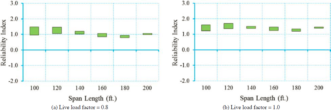
Figure 6-77. Reliability indices for bridges at decompression limit state (ADTT = 5,000).
where
| γL–Operating–Striped = | Live load factors at operating level using number of striped lanes. |
| γL–Operating–Design = | Live load factors at operating level using number of design lanes. |
| MPFStriped = | Multiple presence factor using number of striped lanes. |
| MPFDesign = | Multiple presence factor using number of design lanes. |
| NStriped = | Number of striped lanes. |
| NDesign = | Number of design lanes. |
- Step 3: Obtain the minimum required resistance using the load and resistance factors.
- Step 4: Obtain the existing reliability indices for the sample bridges under the current practices.
- Step 5: Determine target beta for inventory and operating levels. A summary of Step 1 through Step 5 is shown in Table 6-33.
- Step 6: Calibrate the live load factors to target beta. The results of this calibration are provided in Table 6-34.
Example
The team evaluated design examples to illustrate the procedures and verify the live load factors for service limit state at the operating level. A design case of 140-ft span-by-span structure was used. The curb-to-curb deck width is 44.3 ft, and the girder section type is 1800-2. The concrete compressive strength is 8,000 psi. The number of design lanes is calculated as three lanes. The number of striped lanes is assumed to be two lanes. The live load factors for Service III limit state at operating level under the current practice is 0.8. The equivalent live load factors using number of design lanes is calculated as 0.63, which is shown in Table 6-35.
Table 6-33. Current practices and reliability indices.
| Current Practice | Number of Live Load Lanes | Live Load Factors | Existing Beta | Target Beta |
|---|---|---|---|---|
| Inventory Level | Design Lanes | 0.8 | β-Inventory-Existing (1-Year Return Period) | β-Inventory-Target = 1 (1-Year Return Period) |
| Operating Level | Striped Lanes | 0.8 | β-Operating-Existing | β-Operating-Target = 0 |
Table 6-34. Calibration results.
| Evaluation Level | Current Practices | Proposed Practices | ||
|---|---|---|---|---|
| Number of Live Load Lanes | Live Load Factors (current practice) | Number of Live Load Lanes | Live Load Factors (unified with design lanes) | |
| Inventory Level | Design Lanes | γL-Inventory-Design Lanes | Design Lanes | γL-Inventory-Design Lanes |
| Operating Level | Striped Lanes | γL-Operating-Striped Lanes | Design Lanes | γL-Operating-Design Lanes |
Table 6-35. Live load factors for Service III limit state at operating level.
| Evaluation Level | Current Practices | Optional Practices | ||
|---|---|---|---|---|
| Number of Live Load Lanes | Live Load Factors (current practice) | Number of Live Load Lanes | Live Load Factors (unified with design lanes) | |
| Inventory Level | Design Lanes | 0.8 | Design Lanes | 0.8 |
| Operating Level | Striped Lanes | 0.8 | Design Lanes | 0.63 (rounded to 0.65) |
Table 6-36. Statistical information for reliability analysis.
| Parameters | Nominal Value | Bias Ratio (Mean to Nominal) | V | Unit | Remark | |
|---|---|---|---|---|---|---|
| Resistance | Cfsi | 0.7 | 1 | 8.0% | N.A. | fsi = Cfsi*fpu Siriaksorn and Naaman (1980) |
| Cfse | 0.83 | 1 | 8.0% | N.A. | fse = Cfse*fsi Siriaksorn and Naaman (1980) | |
| fpu | 270.0 | 1.03 | 2.0% | ksi | Siriaksorn and Naaman (1980) | |
| e | 43.94 | 1 | 0.0% | in. | Deterministic | |
| Eps | 29,000 | 1.011 | 1.0% | ksi | Siriaksorn and Naaman (1980) | |
| Aps | Inventory Level: 16.0 Operating Level: 13.0 | 1.012 | 1.0% | in.2 | Siriaksorn and Naaman (1980) | |
| Ac | 8,637 | 1 | 2.0% | in.2 | NCHRP Project 12-33 | |
| CEc | 33 | 1.018 | 12.2% | N.A | Siriaksorn and Naaman (1980) | |
| gC | 150 | 1 | 3.0% | lbs/cu ft | Siriaksorn and Naaman (1980) | |
| fc | 8,000 | 1.110 | 11.0% | psi | Nowak (2008) | |
| Dead Load | MD-Beam | 1,903 | 1.03 | 8.0% | k-ft | NCHRP Project 12-33 |
| MD-Barrier | 1,470 | 1.03 | 8.0% | k-in. | NCHRP Project 12-33 | |
| MD-WS | 4,307 | 1.1 | 25.0% | k-in. | NCHRP Project 12-33 (Design 3.175 in., mean 3.5 in.) | |
| Live Load | LL | 1,568 (lane) + 2,243 (truck) | 1.13 | 15.0% | k-ft | NCHRP Project 12-83 1-Year Level |
| IM | HL93 Truckload | 0.1 | 80.0% | N.A. | Nowak 1999 | |
| MPF | AASHTO or New | 1 | 0.0% | N.A. | Deterministic | |
Reliability analysis was performed on these bridges to evaluate the reliability indices for inventory and operating levels. The statistical information used is given in Table 6-36. The minimum required area of prestressing steel is calculated as 16 in.2, and 13 in.2, for inventory level and operating level, respectively. The MPFs developed in this study are given in Table 6-37. The values are accompanied with current AASHTO LRFD values for comparison purposes.
Monte Carlo simulation was used to obtain the statistics about the decompression moment. Then, the reliability index was calculated using the following equation:
| (6-46) |
Table 6-37. Multiple presence factors.
| Number of Lanes | AASHTO LRFD | Values Developed in This Study |
|---|---|---|
| 1 | 1.2 | 1.2 |
| 2 | 1 | 1 |
| 3 | 0.85 | 0.75 |
| 4 | 0.65 | 0.6 |
where
µMDecb, µMLL-Static, and µMLL-IM are the mean values of decompression moment, static live load, and dynamic live load, respectively.
σMDecb, σMLL-Static, and σMLL-IM are standard deviations of decompression moment, static live load, and dynamic live load, respectively.
The results of reliability indices for this example are shown in Table 6-38. For the critical case of three traffic lanes, the reliability indices are about 1.0 and 0.0 for inventory and operating levels, respectively.
6.5.9 Calculation of a Reliability-Based System Redundancy Factor
Redundancy refers to the ability of a structure to support loads beyond first member failure. In other words, the structural system has capacity beyond the resistance of its highest-strength single member. For bridge structures, several commonly recognized forms of redundancy include internal redundancy, where the failure of a single component does not cause additional component failures; structural redundancy, due to the continuity of a given load path; and load path redundancy, due to the existence of multiple supporting components (Ghosn et al. 2014).
The AASHTO’s Standard Specifications for Highway Bridges (2002) required consideration of redundancy in some cases but provided little guidance on how to quantify or implement this requirement. Later, AASHTO LRFD (2020a) introduced the load modifier η, a product of three factors to account for ductility, redundancy, and operational classification, where each factor is given a range from 0.95 to 1.05, depending on bridge characteristics. However, how these factors are defined and implemented is somewhat subjective and open to some interpretation by the designer. The MBE (2019) provides a set of system factors for post-tension segmental construction when considering longitudinal flexure in Table 6A.5.11.6, based on the recommendations of Corven Engineering (2004), which are further discussed.
Ghosn and Moses (1998) proposed a less subjective, quantitative approach to determine system redundancy factors for girder bridges. Four generalized limit states were considered: component failure, ultimate system failure, functionality, and a damaged condition evaluation. Ultimate system failure was defined as the development of a collapse mechanism or when the bridge is damaged to the extent that it is no longer operational. The functionality limit was taken as a deflection exceeding a hundredth of the span length (L/100), while the damaged condition considered ultimate system capacity once a single member is damaged and nonfunctional. To evaluate these limit states, simplified (grillage) FE models of typical girder bridges were constructed and loaded with dead load and two side-by-side HS20 truck configurations, while the load factor (LF) on the trucks was increased until each limit state was exceeded, resulting in limiting load factors for a single component (LF1), the bridge system (LFu), functionality (LFf),
Table 6-38. Reliability analysis results for 140-ft 1800-2 ASBI box beam example (ADTT = 5,000, return period = 1 year).
| Number of Traffic Lanes | Inventory Level | Operating Level | ||
|---|---|---|---|---|
| Existing Reliability Indices | Probability of Exceedance | Existing Reliability Indices | Probability of Exceedance | |
| Single Lane | 4.05 | 2.6E-05 | 3.09 | 0.001 |
| Two Lanes | 1.65 | 0.05 | 0.6 | 0.27 |
| Three Lanes (Critical Case) | 1.06 | 0.14 | 0.04 | 0.49 |
and the damaged system (LFd). It was found that average load factor ratios were as follows: LFu/LF1 = 1.3; LFf/LF1 =1.1; and LFd/LF1 = 0.50. Based on these results, it was proposed that the system factor for a particular bridge be taken as 1.0 if the structure meets these minimum ratios, and the system factor be correspondingly increased or decreased as these ratios increase or decrease, respectively. As an alternative to bridge-specific analysis, a table of results is given for typical girder bridge geometries. In terms of reliability, it was found that the average difference between the reliability index for the system and component was 0.85, 0.25, and −2.70 for the ultimate, functionality, and damaged limit states, respectively. The report notes that unique bridges are best analyzed for redundancy individually rather than using the general, average factors provided.
Expanding on NCHRP Report 406, Ghosn et al. (2014), in NCHRP Report 776: Bridge System Safety and Redundancy, present methods for developing system factors for bridges under lateral and vertical loads. The study determined system factors that would provide the increase in reliability index recommended in NCHRP Report 406 for different bridge geometries and conditions. An objective of this study was to expand the range of bridges considered from minimally designed structures as in NCHRP Report 406, to bridges with over- as well as under-designed members. It should be emphasized that NCHRP Report 406 and NCHRP Report 776 both focused on girder bridges.
Corven Engineering (2004) produced a report for FDOT specifically addressing system factors for segmental bridges, which were later incorporated into the MBE. Here, system factors accounted for redundancy with regard to longitudinal continuity; the continuum behavior of a closed box girder; and multiple post-tensioning tendon paths. The proposed system factors for longitudinal flexure ranged from 0.85 to 1.30 and are given as a function of different types of segmental construction; the expected degree of continuity; the number of girder webs in the section; and the number of prestress tendons per web. Values were primarily based on the performance of existing bridges and judgment. For longitudinal flexure, the system effect was based on the number of plastic hinges required for a failure mechanism. Considering closed box girder behavior, it was noted that, in terms of redundancy, the number of box girder webs is not equivalent to the number of beams on a girder bridge because of the different load-carrying mechanisms of the webs. For example, in torsion, only exterior webs are primarily active, while in shear, more force is carried by a center web, if present; and in flexure, all webs are significantly active. Multiple post-tensioning tendons were also considered as a form of internal redundancy, where additional tension load-carrying paths may increase system factor.
6.5.9.1 Current MBE System Factors for Segmental Bridges
A general discussion of system factors is given in section 6A.4.2.4 of the MBE. A system factor (φs) of 1.0 indicates adequate redundancy, while in no case should φs exceed 1.2. Appropriate system factors for cases not directly addressed may be determined with the process given in NCHRP Report 406 (Ghosn and Moses 1998). However, system factors are not to be applied to shear limit states, as such failures are often brittle and offer no significant ductility. Section 6A.5.11.6 provides specific system factors for segmental bridges, where MBE Table 6A.5.11.6-1 gives factors for post-tensioned segmental concrete box girder bridges considering longitudinal flexure (Table 2-1).
It should be noted that some values in this table may be increased to 1.3, beyond the 1.2 limit specified in 6A.4.2.4. As noted previously, these factors are taken from Corven Engineering (2004). The MBE commentary (C6A.5.11.6) notes that the system factors are meant to account for several aspects of segmental bridge construction, including longitudinal continuity; the integrity of the closed box section; multiple-tendon load paths; multiple webs; and the effect of post-tensioning on certain construction details. Consistent with section 6A.4.2.4 of the MBE, segmental
bridge system factors are taken as 1.0 for shear and torsion, φs is taken as 1.0 for transverse flexure.
6.5.9.2 Origin of Current System Factors for Segmental Bridges
Corven Engineering (2004) and the MBE provide a summary of the background and reasoning behind the specified system factors. For longitudinal flexural behavior, the issues noted previously, which the system factors are meant to address, can be grouped into three considerations: longitudinal continuity, the continuum of the box girder, and multiple tendons.
Longitudinal continuity refers to the need for multiple plastic hinges to form for a continuous multiple-span structure to fail by formation of a mechanism. In Corven Engineering (2004), it was noted that segmental sections were shown to have sufficient stability to form plastic hinges in negative moment regions over supports without local element failure, which may not be true for typical continuous girder bridges, where girders often lack sufficient web compactness (Ghosn and Moses 1998).
The box girder continuum refers to the recognition that localized damage to an external web may occur without severely reducing the overall load-carrying capacity of the segment. For example, the impact from an over-height vehicle may open a hole in an external segmental web that would not cause girder failure, but the same collision may cause a nearly complete loss of capacity for a typical exterior bridge girder.
Multiple tendon load paths consider the effect of tension force redundancy, where the loss of one tendon in a system of tendons becomes less critical as the number of tendons increases.
From these general considerations, the origin of the values given in MBE Table 6A.5.11.6-1 for longitudinal flexure is described as follows.
Based on observations of the adequate performance of existing structures and judgment, a baseline case of φs = 1.0 was given to balanced cantilever bridges at the end spans or interior span with a hinge (i.e., two plastic hinges needed for failure), with two webs and two tendons per web. If only one tendon is provided in the webs, φs was reduced to 0.85.
Considering the results presented in NCHRP Report 406, where Ghosn and Moses (1998) suggested that system factors for box beam bridges were similar to those of I-beam girder bridges when treating each web as an I-beam, system factors were taken as 1.10 and 1.20 for simple span and continuous segmental spans, respectively. For segmental bridges, Corven Engineering (2004) assumed that these factors would apply to typical two-web sections of the most redundant type that have four or more tendons per web. For the case of sections with three webs, a system factor increase of 0.10 was assumed, to account for an increase in section integrity and additional load paths. System factors for sections with intermediate characteristics were developed from interpolation.
When the transverse direction was considered, the deck of the segmental section offered no redundancy over a routine prestressed concrete flexural member, and thus, φs = 1.0. Because of the generally non-ductile/non-redundant nature of shear and torsion failures, the system factor was also taken as 1.0 for these failure modes. The system factor was taken as 1.0, when local shear and/or strut and tie behavior were considered, and local post-tensioning was used for the case of two or more tendons or bars providing resistance. The system factor was reduced to 0.90 for the case of one tendon or bar providing resistance.
6.5.9.3 System Factor Revision Process
The revision process follows the conceptual approach as described in NCHRP Report 406 (Ghosn and Moses 1998). In this approach, system factors are based on the redundancy ratios
of system to component capacity. For girder bridges, a component is defined as an individual girder. However, the definition of a component must be reconsidered when segmental bridges are analyzed. From the previous discussion for longitudinal flexure, the existing segmental bridge system factors are meant to account for three types of behavior: longitudinal continuity, the integrity of the box section, and multiple tendon paths. As such, components must be defined to recognize these effects. In terms of longitudinal continuity, a component is a potential plastic hinge necessary for bridge failure; for section integrity, a component is an individual web; and when considering multiple tendon load paths, a component is a tendon. The proposed process to develop system factors for longitudinal flexure is as follows:
- Select representative bridges. A small number of representative, hypothetical structures is selected that considers the following parametric variations: span-by-span and cantilever construction; degree of longitudinal continuity (one, two, three plastic hinges until failure); number of webs (two, three); and number of tendons per web (one, two, three, four).
- Load a considered structure with dead load and with the expected live load overload configuration. Based on the available load data, this is expected to be two side-by-side trucks. However, some single-lane cases were analyzed as well. Following the NCHRP Report 406 approach, the vehicles are idealized into HS20 configurations (Ghosn and Moses 1998).
2.1. Conduct first component failure analysis. The live load is increased on the structure until a component failure occurs. Component failure is defined as follows:
- Initiation of a plastic hinge
- Tendon failure
- Shear failure of a web
Note that (a) is taken as either tendon yielding or concrete crushing at a plastic hinge location, whichever occurs first; and for (b), tendon failure is taken as tendon yielding. Thus, there is some potential overlap in component failure states for (a) and (b).
The live load factors needed to cause each component failure are recorded (LF1).
2.2. Conduct system capacity analysis. The live load on the structure is increased until the peak load that the structural system can carry is determined. This is associated with the formation of one or more full plastic hinges (i.e., concrete crushing, a tendon reaching ultimate stress, or excessively large deformations thought to jeopardize structural integrity, such as that approaching the depth of the section). The live load factor needed to cause system failure is recorded (LFu). The analysis is repeated, but now system capacity is redefined with a functionality limit, given in terms of deflection (LFf). In NCHRP Report 406, the deflection limit was taken as span/100 (Ghosn and Moses 1998). This limit was found to be reasonable for segmental bridges as well and was used in this study.
- Load factor ratios (redundancy factors) corresponding to the ultimate strength and functionality, respectively, are computed: LFu/LF1 and LFf/LF1.
- The damaged system is now considered. Step 2.2 is repeated, but before determining the load factors, a component is first damaged after LF1 is computed in the undamaged state. The type of damage is dependent on the type of component considered:
- Insertion of a full plastic hinge (i.e., removal of the moment-carrying capability of a hinge point).
- Weakening a portion of a web by removing its shear-carrying capability.
- Removal of a tendon to simulate tendon rupture.
The live load factor corresponding to the ultimate damaged system capacity was then determined (LFd), and the load factor ratios corresponding to ultimate damaged strength were calculated: LFd/LF1.
- Record the final redundancy factors for the ultimate (Rult), functionality (Rdef), and damaged (Rdam) states: Rult = LFu/LF1; Rdef = LFf/LF1; Rdam = LFd/LF1).
- Convert redundancy factors to system factors. Adequate redundancy is achieved if the structure has ratios LFu/LF1, LFf/LF1, and LFd/LF1 of 1.3, 1.10, and 0.50, respectively. These are associated with changes in component-to-system reliability of +0.85, +0.25, and −2.7, respectively. A structure exactly meeting these criteria is given a system factor of 1.0. The conversion process from redundancy to system factors is as follows:
- Compute reliability index using resistance equal to that which caused the first component failure. Vehicular live load is to be based on a 75-year return period for ultimate and deflection limits and a 2-year return period for damage consideration.
- Compute reliability index using resistance equal to that which caused the system failure (i.e., at load levels LFu, LF1, and LFd). Mean system resistance can be determined by multiplying the mean resistance at first component failure resistance by the redundancy factor for the case investigated. Following the approach given in NCHRP Report 406, it is conservatively assumed that system coefficient of variation is unchanged from that of the component.
- Determine the factor needed to be applied to the system resistance such that the case investigated results in a change in reliability from the component level to the system level equal to the level of change given in Step 6 (i.e., either +0.85, +0.25, or −2.7). Here it is assumed that the initial component reliability is close to 3.5; otherwise, the expected reliability index changes may require adjustment to achieve corresponding changes in failure probability. The inverse of the required factor to be applied to the system resistance is the system factor.
6.5.9.4 Modeling Approach
Due to the need to consider the damaged state, where system behavior considers localized web damage or the removal of a single tendon, analytical approaches become difficult to implement, and a finite element procedure is used.
Concrete Model
Concrete was modeled with the concrete damaged plasticity (CDP) approach, which is described in detail elsewhere (see, for example, Genikomsou and Polak 2015). Primary model parameters are ψ, the dilation angle (in the p-q plane) at high confining pressure and accounts for changes in Poisson ratio as pressure increases; k, the ratio of deviatoric stresses in uniaxial tension and compression, which varies from 0.5 when using a Rankine yield surface to 1.0 when using von Mise theory; ε, the eccentricity of the plastic potential surface; fb0/fc0, the ratio of initial biaxial to uniaxial compressive yield stress; and µ, the viscosity parameter, which is used to increase numerical convergence by allowing stresses to extend beyond the specified yield surface. For this research, the following values were used: ψ = 31; ε = 0.1; fb0/fc0 = 1.16; k = 0.667; and µ = 0 (Kupfer et al. 1969; Lubliner et al. 1989; Ren et al. 2015; Genikomsou and Polak 2015). The concrete considered had assumed properties: compressive strength fc′ = 7 ksi; Young’s Modulus E = 4,770 ksi; and Poisson ratio v = 0.19.
Within the CDP model, concrete compressive response was taken from Hognestad (1951), as shown in Figure 6-78, while the tension response was taken from Vecchio and Collins (1986) and shown in Figure 6-79.
The prestress steel model (Figure 6-80) is based on that of Devalapura and Tadros (1992), where Grade 270 low relaxation strands are considered. Curve constants are taken as A = 887; B = 27613; C = 112.4; and D = 7.36 for 0.9fpy/fpu strands. The stress-strain relationship for mild steel bars (Grade 60) was taken as bilinear.
6.5.9.5 Span-by-Span Structure Considered
The span-by-span case considered is based on the structure detail in the rating examples (Appendix C of the Guideline) and is summarized here, with the geometry given in Figure 6-81.

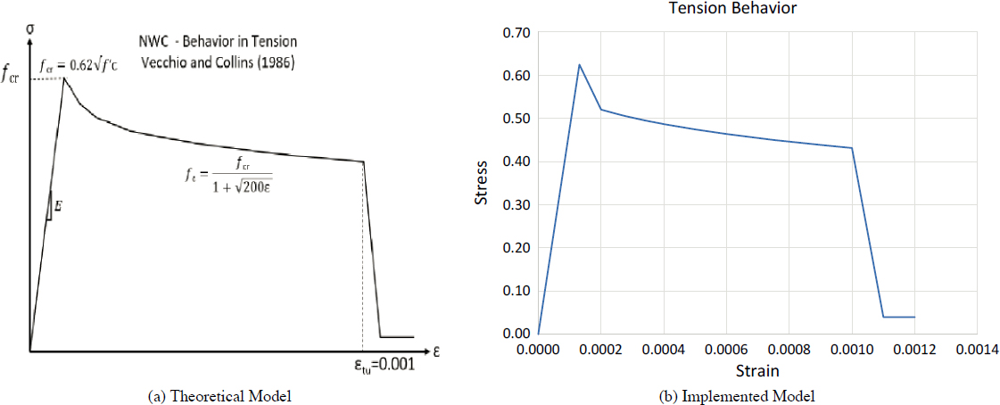
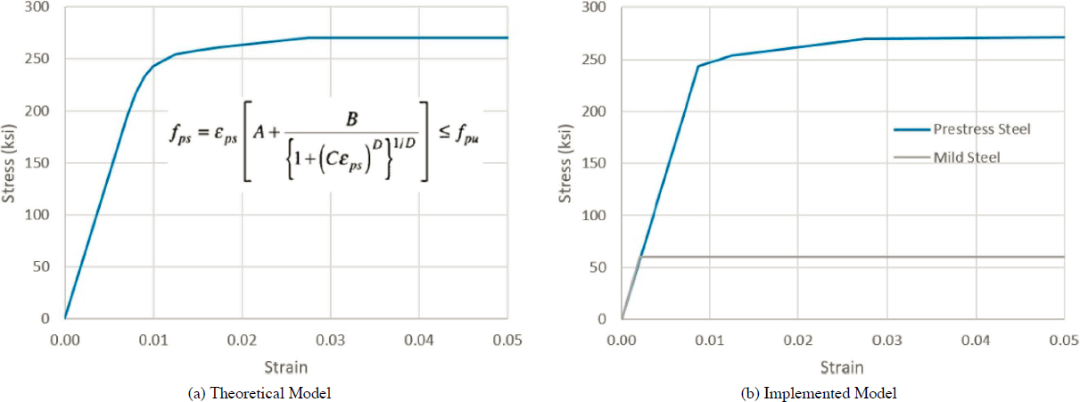
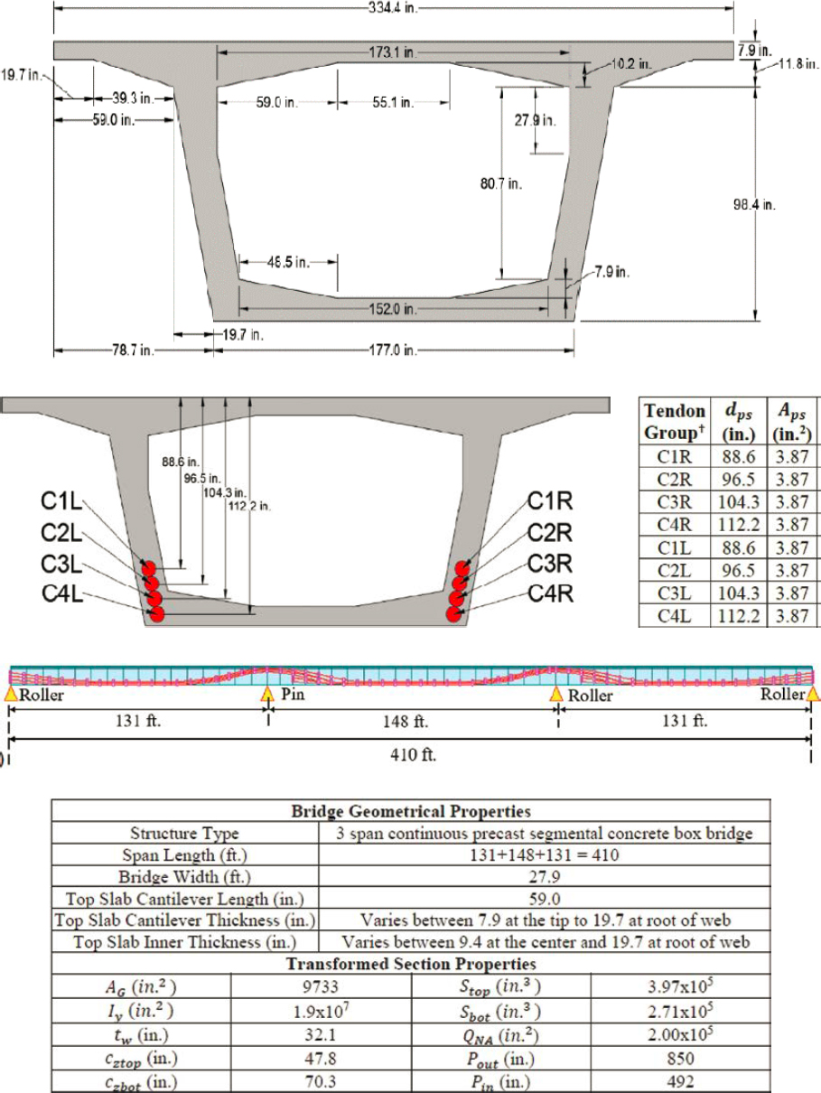
This three-span structure has four tendons per side, where each tendon has a total prestress steel area of 3.87 in.2, for a total prestress steel area of 30.96 in.2. In the finite element analysis (FEA) model, tendons were stressed to an effective prestress of 173 ksi. The total effective prestress force is 5,363 k (670k per tendon).
6.5.9.6 Span-by-Span FEA Model Geometry
A model composed of shell elements was initially constructed and validated to the expected single-span load-displacement response developed from the theoretical moment-curvature diagram. Although this model initially produced good results, it also produced numerical difficulties when staged construction was considered. Therefore, a solid element alternative model was developed.
The solid element model employed linear hexahedral elements (reduced integration, enhanced hourglass control) to represent concrete and discrete truss elements for prestress and mild steel. A mesh density and element type study was conducted, and it was found that the model used represented a reasonable balance between accuracy and computational efficiency. This model is illustrated in Figure 6-82. The model includes transverse prestress tendons in the top flange and vertical bars in the webs.
The load-deflection response of the single-span model was compared to a moment-curvature analysis of a simplified form of the structure (i.e., assuming one layer of steel at the tendon centroid and rectangular flange and web components with average thickness). Good agreement was obtained, as shown in Figure 6-83. Once validated, two-span and three-span versions of the model were constructed, as shown in Figure 6-84 and Figure 6-85.


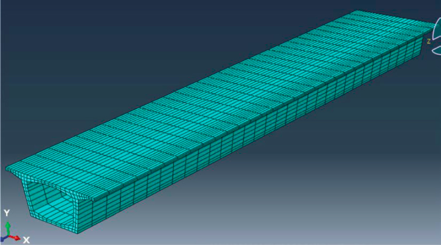
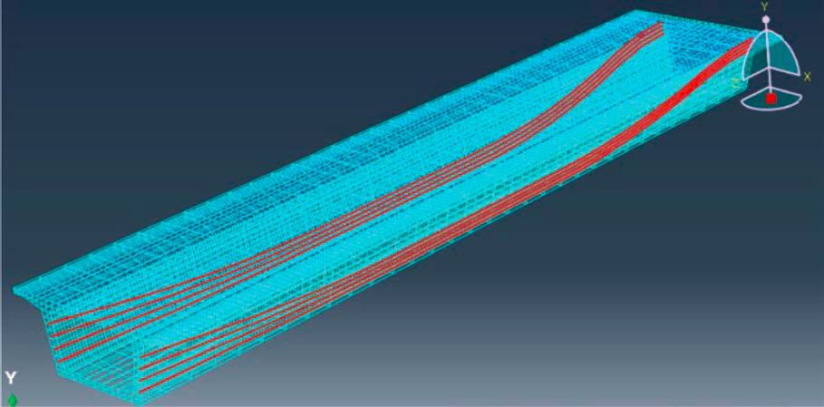
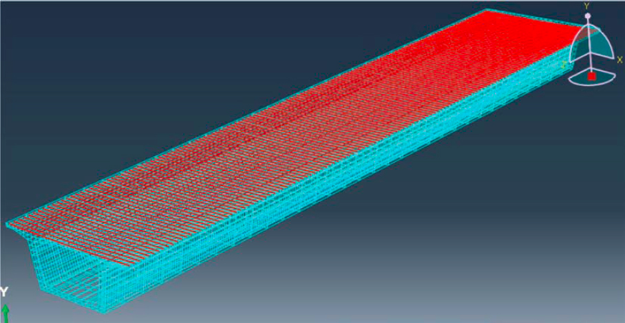
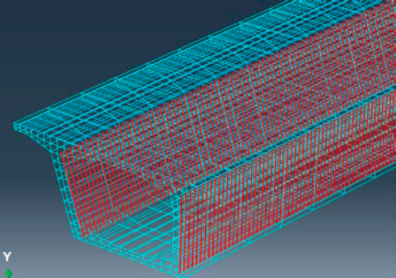

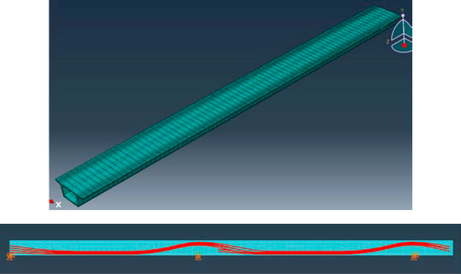
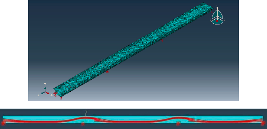
6.5.9.7 Analysis Process
The model was implemented in Abaqus. When subjected to large deformations and significant softening due to cracking near ultimate capacity, the CDP model produces a highly nonlinear response that could not be effectively solved with an implicit solver due to convergence difficulties. Therefore, the model was solved with a more costly but viable explicit solution. For the prestress and dead load stages, where the response was essentially linear, a total step time of T = 20 seconds was used, while for the subsequent live load incrementation stage wherein the structure was brought to ultimate capacity, a time of T = 100 was used. In the modeling process, self-weight is simulated with a gravity (body) load, and prestressing was simulated by applying an appropriate temperature change to the tendons.
Ideally, to determine the effect of the construction process on system behavior, the complete segment-by-segment sequential construction process, with associated changes in prestress over time throughout the structure, could be simulated. However, this represents a high degree of modeling complexity and computational time when implemented in 3D FEA models as used here. As an approximation to explore this effect, a simplified span-by-span staged construction process was considered and modeled as follows:
First Stage.
The first span is activated, supported by its end supports, and then loaded with dead load and prestress forces applied simultaneously. As the structure is within its linear elastic range under this load combination, the order of load application at this point is not important and applying dead load and prestress simultaneously avoids the need to add additional temporary supports to support the beam under dead load prior to application of prestress to avoid beam cracking.
Second Stage.
The second span is activated, where one end is linked to the first span, and the far end is supported by its support. It is then loaded with dead load and prestress forces simultaneously, similar to the first span. This sequence assumes that the joint between the beams carried dead load in addition to live load stresses (i.e., essentially, that the second span is temporarily supported in the construction process, such as from a crane, until the beam is joined to the first span via prestressing tendons).
Third Stage.
The second stage is repeated for the third span.
Fourth Stage.
Once the beam is completely linked, prestressed, and subjected to its self-weight, live load is applied and incremented upward until the complete load-displacement response of the structural system is obtained. Following the process outlined in NCHRP Report 406, the live load was applied in the form of two side-by-side HS20 truck configurations (Ghosn and Moses 1998). Truckloads are placed on the span(s) to generate maximum positive moment effect. In one case, trucks are placed on a single span, whereas in the second case, trucks are placed on two adjacent spans, as shown in Figure 6-86. In select cases, the effect of lateral truck position and the use of a single truck were investigated.
This process was simplified from many alternative construction approaches and was initially chosen for computational feasibility. Based on the results, however, as summarized below, modeling more complex construction sequences was not further pursued for purposes of estimating system factor.
The redundancy (and thus system) factors for this staged construction process were compared to those using a simplified two-stage process for the entire structure, where first, the complete structure was joined together and then subjected to dead load and prestress (i.e., practically assuming that the entire structure was cast-in-place at once), then the structure was subjected to live load.
During this comparison, several different prestress levels, to account for variations in losses and initial design assumptions, were also explored in both modeling approaches. Prestress was varied by up to 20%, and taken as constant throughout both spans. Also, the expected effective prestress force was changed from one span to the next by up to a difference of 20%. Initial analyses revealed that redundancy factor Rult showed little variation (less than 5%) regardless of the modeling approach or change in prestress level used, within the range considered. This is perhaps not surprising, since redundancy factors are computed at high load levels, within a structural response range from first tendon yielding to ultimate system capacity. At such load levels, well beyond that which indicates decompression and flexural cracking, the initial service level stresses lose significance. Additional subsequent analyses, however, indicated that redundancy factor can be sensitive to variation in tension steel parameters in some cases, particularly when changes in prestress level and steel area are considered. Decreasing prestress force and increasing prestress steel area tend to decrease redundancy factor for some structures and load scenarios. In contrast, it was found that Rdef was affected significantly by changing prestress, by roughly the same proportion that prestress force was changed. However, the system factor corresponding to Rdef rarely governed in any case [see Tables 6-43(a) and 6-43(b)]. Thus, for
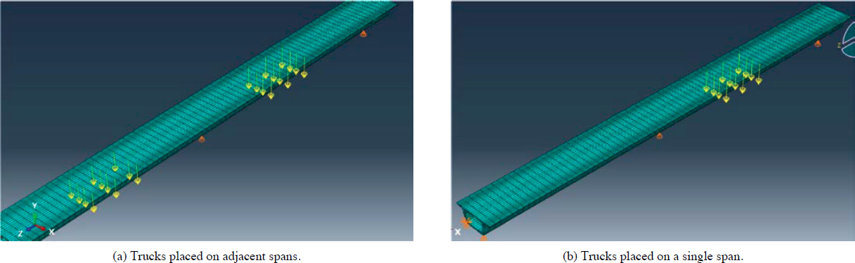

development of system factors, the simplified two-stage model was used, and effective prestress losses were taken as approximately 15% of the initial prestress force uniformly throughout all spans.
An example load-displacement curve for a two-span structure with both spans loaded is shown in Figure 6-87. In Figure 6-88, the load-stress curve associated with the top prestress tendon over the central support is shown. The vertical axis on the diagram represents the sum of all reactions due to self-weight in addition to live load (i.e., the total vertical load on the structure).

The self-weight of the structure is approximately 3,000 kips; it is at this point in the figure that application of the live load begins. Note that the load-deflection response prior to this point should not be taken to represent the behavior of the actual structure because the response shown is due to the simultaneous, incremental application of dead load and prestressing force (thus stiffness prior to 3,000 kips cannot be obtained from the figure). The result of this artificial loading can also be seen in Figure 6-88, with the increase in tendon stress from zero to approximately 170 ksi once the stage 1 loading has ended. In Figure 6-87 and Figure 6-88, Point A is the onset of tendon yield (243 ksi), while Point B is the onset of large deformation, where the stiffness of the structure approaches zero, relative to prior stiffness in the loading history. Practically, this can be taken as the system capacity limit. In Figure 6-87, Point C is the deflection limit of L/100 (i.e., approximately 15.7 in. for a 131-ft span).
Example deflected shapes (deformations magnified for visibility) for the two-span structure with one span loaded (Figure 6-89), two spans loaded (Figure 6-90), and for the three-span structure with both spans loaded (Figure 6-91) are shown for comparison. As seen in the figures, a large loss of stiffness appears concentrated near the high moment points (i.e., near midspan and the central supports), forming localized plastic hinges, whereas the remainder of the span remains relatively stiff. These localized areas of largest stiffness loss are expected, as significant cracking and thus large curvatures occur where moments are greatest.
To explore the effect of changing the section length/depth ratio (L/d), additional versions of the two- and three-span structures were considered, where the section geometry was unchanged but the length was increased, and prestress steel area and initial prestress level were correspondingly changed accordingly to produce feasible designs. Here, the original L/d ratio of approximately 15 (for the longest span) was increased to approximately 24. An even more slender version was also modeled (L/d approaching 30), but no significant differences in results were obtained from the L/d ≈ 24 case.
To determine the effect of the number of tendons when tendon damage was considered, models similar to the four tendon per web case were constructed but using three, two, and one tendon per web. Tendon damage was implemented by removing one tendon in one web. For multiple spans, cases removing either a positive moment tendon or a negative moment tendon were considered. To explore the effect of web damage, a hole was inserted into one web. Hole


dimensions were taken as the entire web height and with a width equal to half of the web height. Transverse (shear) steel within the hole was removed, but tendons that passed through the hole were not damaged. Two cases were considered: the hole placed at midspan and the hole placed at the critical section as determined by AASHTO LRFD (2020a) shear design provisions. The latter resulted in a hole close to a support. An example web damage case is given in Figure 6-92. In these damage cases, trucks were placed longitudinally such that the center axle was centered over the hole. For all damage cases (tendon or web damage), trucks were offset laterally to the extent specified by AASHTO LRFD (2020a), to the side of the bridge where damage was implemented.
6.5.9.8 Three-Web Structure
To explore the effect of changing the number of webs, a three-web, 195-ft, two-celled section was modeled, based on the longest span of the Port of Miami/Dodge Island Bridge. This section has a total width of 53 ft and a section height of 111 in. (L/d ≈ 21). The FEA model is shown in Figure 6-93.

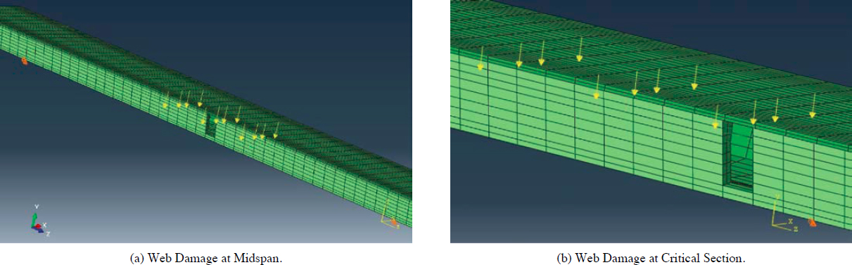
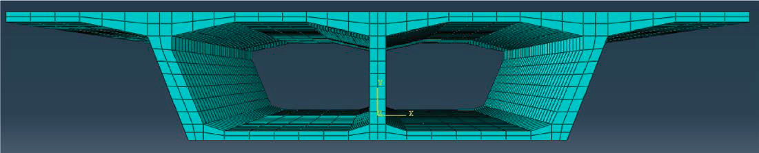
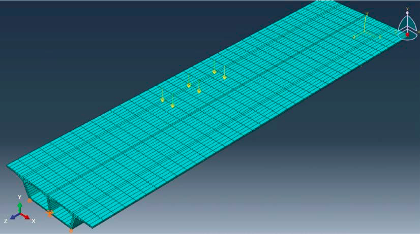
6.5.9.9 Non-Prismatic, Balanced Cantilever Structure Considered
The balanced cantilever case considered is described in detail in the rating examples and is summarized here, with the three-span geometry based on that shown in Figure 6-94.
This three-span structure has single cell symmetric concrete segments with a varying depth between 275.5 in. to 106.2 in. The total span length is 984 ft, and the width of the segments is 42 ft. The bottom flange thickness of the segments from pier to midspan decreases from 33.5 in.

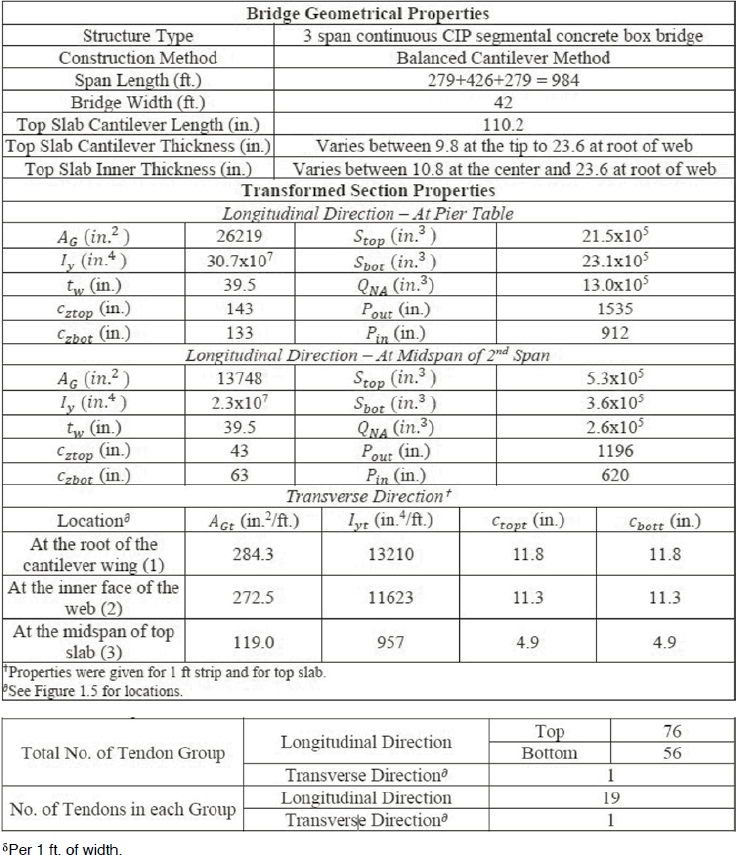
to 10.2 in. The thickness of the top flange varies from 9.8 in. at the tip to 23.6 in. at the root of the web.
The structure was modeled and analyzed using the same approach as described for the span-by-span case. The three-span model is shown in Figure 6-95.
6.5.9.10 Results
Bridge Reactions
The modeling approach discussed was used to determine the load on the bridge corresponding to the limits of system capacity, functionality, first component failure, and damage. Table 6-39 presents the sum of bridge vertical reactions that correspond to ultimate system capacity; a deflection limit of L/100 (functionality); and first component failure. Both total reactions, including dead load (L + D) and live load only reactions (L) are provided. The latter were extracted from (L + D) reactions and were used to compute redundancy factors, as previously discussed. Note that in all cases, first component failure occurred with tendon yielding rather than web failure or concrete crushing. This was expected given the tension-controlled designs considered.
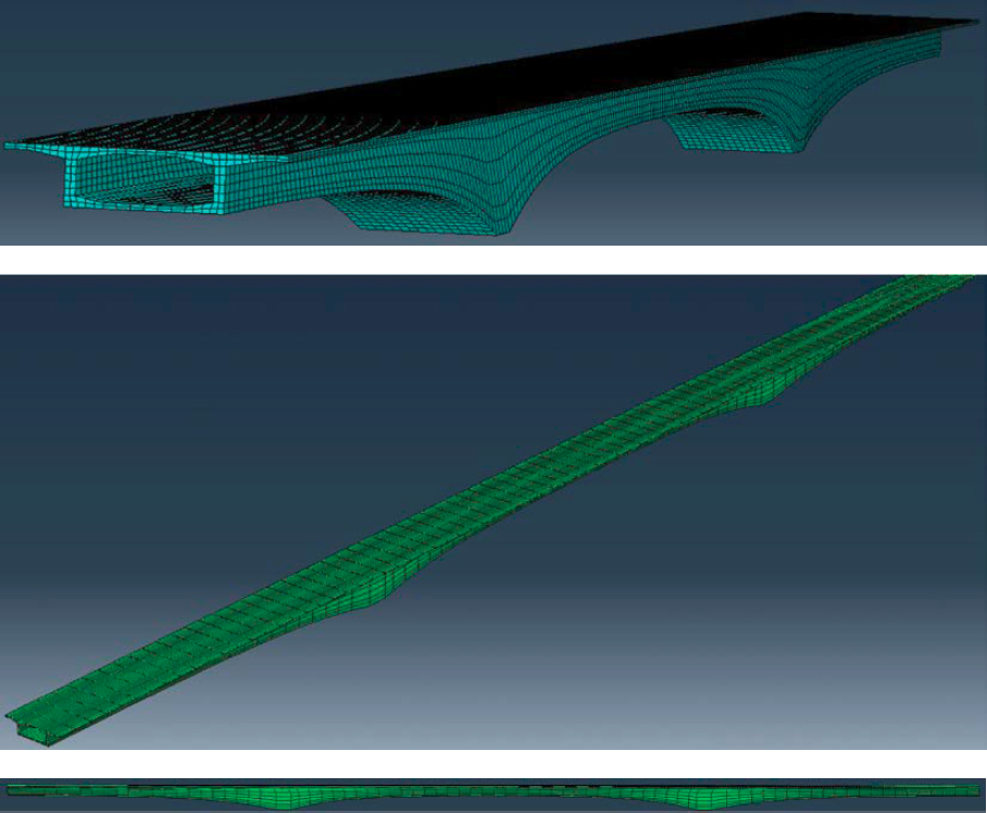
In the table, results are presented for several different truckload positions; two side-by-side trucks centered in their lanes at the maximum positive moment positions placed on either one or two adjacent spans; two side-by-side trucks placed eccentrically on the bridge on one span, moved as close to the edge of the design lanes as specified by AASHTO LRFD (2020a), assuming a barrier width of 1.5 ft; and one truck placed eccentrically on the bridge. For the single-span loaded cases, trucks were placed on the longest (central) span. For the case where trucks were placed on adjacent spans (both spans loaded), an alternative location was studied where trucks were placed at locations to maximize negative moment at the support rather than positive moment at the midspans. This alternative case resulted in a slightly higher redundancy factor (by about 5%) and thus was not considered further.
Table 6-40 and Table 6-41 present ultimate capacity reactions that correspond to the tendon-damaged system. Here, one tendon was removed in one web before loading the structure. In general, this was the tendon with the greatest depth in the positive moment region (i.e., lowermost tendon). The effect of removing a negative moment tendon was also considered in several test cases, and it was found that the loss of the positive moment tendon governed. For the three-web case, a tendon on the outermost web was removed. In all cases, trucks were positioned near the side of the bridge where the tendon was removed, which was found to produce the lowest redundancy factors.
Table 6-42 presents ultimate capacity reactions that correspond to the web-damaged system. Here, a portion of the web was removed either at midspan or at the critical section, and trucks were placed to the side of the bridge with the damaged web. Additional details on web damage and live load application in this case were discussed previously.
Table 6-39(a). Span-by-span bridge reactions (kips).
| Ultimate System Limit | Deflection L/100 | 1st Comp. Failure | ||||
| L + D React | L React | L + D React | L React | L + D React | L React | |
| 1 Span/Hinge to Failure (L/d = 15) | ||||||
| Trucks Symmetric | 3,322 | 2,024 | 3,065 | 1,767 | 2,831 | 1,533 |
| Trucks Offset | 3,179 | 1,881 | 3,012 | 1,714 | 2,745 | 1,447 |
| Single Truck Offset | 3,147 | 1,849 | 2,973 | 1,675 | 2,744 | 1,446 |
| 1 Span/Hinge to Failure, 3-Web Section (L/d = 21) | ||||||
| Trucks Symmetric | 4,498 | 1,448 | 4,341 | 1,291 | 4,115 | 1,065 |
| Trucks Offset | 4,263 | 1,213 | 4,264 | 1,214 | 4,080 | 1,030 |
| Single Truck Offset | 4,249 | 1,199 | 4,148 | 1,098 | 4,093 | 1,043 |
| 2 Span/Hinges to Failure (L/d = 15) | ||||||
| 1 Span Loaded | ||||||
| Trucks Symmetric | 5,304 | 2,262 | 5,001 | 1,959 | 4,658 | 1,616 |
| Trucks Offset | 5,326 | 2,284 | 4,965 | 1,923 | 4,666 | 1,624 |
| Single Truck Offset | 5,203 | 2,161 | 5,050 | 2,008 | 4,536 | 1,494 |
| 2 Spans Loaded | ||||||
| Trucks Symmetric | 7,839 | 4,797 | 7,221 | 4,179 | 6,764 | 3,722 |
| Trucks Offset | 7,218 | 4,176 | 7,186 | 4,144 | 6,113 | 3,071 |
| 2 Span/Hinges to Failure (L/d = 24) | ||||||
| 1 Span Loaded | ||||||
| Trucks Symmetric | 6,284 | 1,706 | 6,230 | 1,652 | 5,838 | 1,260 |
| 2 Spans Loaded | ||||||
| Trucks Symmetric | 8,412 | 3,834 | 8,173 | 3,595 | 7,942 | 3,364 |
| 2 Span/Hinges to Failure (L/d = 30) | ||||||
| 1 Span Loaded | ||||||
| Trucks Symmetric | 7,007 | 1,230 | 6,884 | 1,107 | 6,665 | 888 |
| 2 Spans Loaded | ||||||
| Trucks Symmetric | 8,494 | 2,717 | 8,406 | 2,629 | 8,098 | 2,321 |
| 3 Span/Hinges to Failure (L/d = 15) | ||||||
| 1 Span Loaded | ||||||
| Trucks Symmetric | 7,021 | 2,943 | 6,650 | 2,572 | 5,928 | 1,850 |
| Trucks Offset | 7,080 | 3,002 | 6,701 | 2,623 | 5,981 | 1,903 |
| Single Truck Offset | 7,030 | 2,952 | 6,599 | 2,521 | 5,933 | 1,855 |
| 2 Spans Loaded | ||||||
| Trucks Symmetric | 10,121 | 6,043 | 9,424 | 5,346 | 8,412 | 4,334 |
| Trucks Offset | 9,860 | 5,782 | 9,311 | 5,233 | 7,933 | 3,855 |
| 3 Span/Hinges to Failure (L/d = 24) | ||||||
| 1 Span Loaded | ||||||
| Trucks Symmetric | 9,437 | 3,108 | 8,868 | 2,539 | 8,471 | 2,142 |
| 2 Spans Loaded | ||||||
| Trucks Symmetric | 11,846 | 5,517 | 11,562 | 5,233 | 10,629 | 4,300 |
Table 6-39(b). Balanced cantilever bridge reactions (kips).
| Ultimate System Limit | Deflection L/100 | 1st Comp. Failure | ||||
| L + D React | L React | L + D React | L React | L + D React | L React | |
| 3 Span/Hinges to Failure | ||||||
| 1 Span Loaded | ||||||
| Trucks Symmetric | 22,053 | 5,375 | 21,352 | 4,674 | 20,427 | 3,749 |
| Trucks Offset | 21,876 | 5,198 | 21,047 | 4,369 | 20,217 | 3,539 |
| 2 Spans Loaded | ||||||
| Trucks Symmetric | 24,950 | 8,272 | 24,163 | 7,485 | 23,891 | 7,213 |
Table 6-40. Bridge reactions with tendon damage (two-web case).
| 4 tendons/web | 3 tendons/web | 2 tendons/web | 1 tendon/web | |||||
| L+D React | L React | L+D React | L React | L+D React | L React | L+D React | L React | |
| 1 Span/Hinge to Failure (L/d = 15) | ||||||||
| Trucks Symmetric | --- | --- | --- | --- | 2,525 | 1,227 | --- | --- |
| Trucks Offset | 2,782 | 1,484 | 2,623 | 1,325 | 2,368 | 1,070 | 2,066 | 768 |
| Single Truck Offset | 2,644 | 1,346 | 2,486 | 1,188 | 2,235 | 937 | 1,731 | 433 |
| 2 Span/Hinges to Failure (L/d = 15) | ||||||||
| 1 Span Loaded | ||||||||
| Trucks Offset | 5,075 | 2,033 | 4,993 | 1,951 | 4,851 | 1,809 | 4,221 | 1,179 |
| Single Truck Offset | --- | --- | --- | --- | 4,761 | 1,724 | --- | --- |
| 3 Span/Hinges to Failure (L/d = 15) | ||||||||
| 1 Span Loaded | ||||||||
| Trucks Offset | 6,668 | 2,590 | 6,540 | 2,462 | 6,088 | 2,010 | 5,433 | 1,355 |
Table 6-41. Bridge reactions with tendon damage (three-web case).
| 2 tendons/web | 1 tendon/web | |||
| L+D React | L React | L+D React | L React | |
| 1 Span/Hinge to Failure, 3-Web Section (L/d = 21) | ||||
| Single Truck Offset | 3,838 | 795 | 3,417 | 367 |
Table 6-42. Bridge reactions with web damage (two-web case).
| At Midspan | At Crit Section | |||
| L+D React | L React | L+D React | L React | |
| 1 Span/Hinge to Failure (L/d = 15) | ||||
| Trucks Offset | 2,670 | 1,372 | 4,085 | 2,787 |
| 2 Span/Hinges to Failure (L/d = 15) (one span loaded) | ||||
| Trucks Offset | 5,052 | 2,010 | 6,017 | 2,975 |
| 3 Span/Hinges to Failure (L/d = 15) (one span loaded) | ||||
| Trucks Offset | 6,940 | 2,862 | 7,800 | 3,722 |
Only some combinations of load position, damage, and bridge geometry were considered. Cases were not quantified when it was apparent that these would not govern. This was particularly so when the three-web and balanced cantilever bridges were considered, where only a small number of cases were analyzed, based on the span-by-span results.
Redundancy Factors
As presented in Table 6-43 through Table 6-45, redundancy factors were calculated using the process described. Using the reaction data given in Table 6-39 through Table 6-42, ratios are computed that represent redundancy factors corresponding to the ultimate strength (Rult), functionality (Rdef), and damage (Rdam), respectively: Rult = LFu/LF1, Rdef = LFf/LF1, and Rdam = LFd/LF1. Here, LF1 is the live load factor (LLF) applied on the HS20 trucks to cause first component failure; LFf is the LLF needed to cause a deflection of L/100; LFu is the LLF for the undamaged
Table 6-43(a). Span-by-span redundancy factors.
| Rult | Rdef | |
| 1 Span/Hinge to Failure (L/d = 15) | ||
| Trucks Symmetric | 1.32 | 1.15 |
| Trucks Offset | 1.30 | 1.18 |
| Single Truck Offset | 1.28 | 1.16 |
| 1 Span/Hinge to Failure, 3-Web Section (L/d = 21) | ||
| Trucks Symmetric | 1.36 | 1.21 |
| Trucks Offset | 1.18 | 1.18 |
| Single Truck Offset | 1.15 | 1.05 |
| 2 Span/Hinges to Failure (L/d = 15) | ||
| 1 Span Loaded | ||
| Trucks Symmetric | 1.40 | 1.21 |
| Trucks Offset | 1.41 | 1.18 |
| Single Truck Offset | 1.45 | 1.34 |
| 2 Spans Loaded | ||
| Trucks Symmetric | 1.29 | 1.12 |
| Trucks Offset | 1.36 | 1.35 |
| 2 Span/Hinges to Failure (L/d = 24) | ||
| 1 Span Loaded | ||
| Trucks Symmetric | 1.35 | 1.31 |
| 2 Spans Loaded | ||
| Trucks Symmetric | 1.14 | 1.07 |
| 2 Span/Hinges to Failure (L/d = 30) | ||
| 1 Span Loaded | ||
| Trucks Symmetric | 1.39 | 1.25 |
| 2 Spans Loaded | ||
| Trucks Symmetric | 1.17 | 1.13 |
| 3 Span/Hinges to Failure (L/d = 15) | ||
| 1 Span Loaded | ||
| Trucks Symmetric 1.59 1.39 | ||
| Trucks Offset | 1.58 | 1.38 |
| Single Truck Offset | 1.59 | 1.36 |
| 2 Spans Loaded | ||
| Trucks Symmetric | 1.39 | 1.23 |
| Trucks Offset | 1.50 | 1.36 |
| 3 Span/Hinges to Failure (L/d = 24) | ||
| 1 Span Loaded | ||
| Trucks Symmetric | 1.45 | 1.19 |
| 2 Spans Loaded | ||
| Trucks Symmetric | 1.28 | 1.22 |
Table 6-43(b). Balanced cantilever redundancy factors.
| Rult | Rdef | |
| 3 Span/Hinges to Failure | ||
| 1 Span Loaded | ||
| Trucks Symmetric | 1.43 | 1.25 |
| Trucks Offset | 1.47 | 1.23 |
| 2 Spans Loaded | ||
| Trucks Symmetric | 1.15 | 1.04 |
ultimate system capacity; and LFd is the LLF for the damaged ultimate system capacity. These values can be determined as follows:
| (6-47) |
| (6-48) |
| (6-49) |
| (6-50) |
Where R1 = total bridge reactions at first component failure; RDL = total bridge reactions due to dead load only; RHS20 = total bridge reactions due to dead load and nominal HS20 vehicle loads on the bridge; Ru = total bridge reactions at ultimate system capacity; Rf = total bridge reactions at the functionality deflection limit of L/100; and Rd = total bridge reactions of the damaged bridge at ultimate capacity.
In the analysis, the definitions of component failure (generally first tendon yield) and ultimate capacity (practically, the peak of the load-deflection curve, but not taken beyond full plastic hinging nor excessively large deformation) were defined previously and are used here. There were no web shear failures in the analyses prior to tendon yield or ultimate flexural capacity.
For multiple-span cases, redundancy ratios are given for the application of trucks on a single (center) span as well as on two adjacent spans, for both laterally symmetrically placed and laterally offset trucks. A single offset truck was also considered. As shown in the tables, results are generally similar whether trucks are offset or symmetrically placed, with differences within 5% for most cases and within about 10% for all cases. This similarity is in part due to the high torsional stiffness of the section, which results in minimal twisting for asymmetric loading. However, loading either one or two spans with trucks did result in significant differences. It was found that loading both spans often results in significantly lower redundancy ratios than when a single span was loaded, as shown in the tables. Loading two spans can cause the critical section to shift to the negative moment region, though this will depend on how the trucks are positioned on the spans. However, as soon as tendons begin to yield in negative moment, stresses increase in the positive moment tendons, and they yield as well. When both spans are loaded, the positive and negative moment failures are usually very close together and are practically simultaneous. When a single span is loaded, however, a larger increment in load is necessary to fail the negative moment region after yielding occurs in the positive moment region. This larger load increment results in the larger redundancy factor for single-span loading. Loading both spans results in a smaller difference between the positive and negative moments on the span, resulting in a smaller load increment between positive and negative region failures, and a lower redundancy factor.
For the three-web structure, only the single-span case was considered. This was because the single-span case, as expected, produced the governing, lowest redundancy factors for the two-web, shorter span structure, and a clear pattern of increasing redundancy factors emerged as the number of spans and thus redundancy increased. Thus, additional multi-span runs for the longer structure were deemed unnecessary. Although the redundancy ratio for the single truck offset case is lower for the three-web structure than for the two-web structure, this is attributed to the increased width of the structure, which is nearly twice as wide as the original (L/d = 15) structure as well as its greater L/d ratio (21).
For the balanced cantilever case, because the trends in redundancy factors with respect to load placement were similar to that of the span-by-span structure, only a few selected cases were considered. Redundancy factors were generally similar to those of the L/d = 24 three-span structure
when one span is loaded, but interestingly lower when two spans are loaded. This appears to follow the general trend of decreasing redundancy with increasing L/d ratio. The cause of this appears to be the relatively high flexibility of the cantilever bridge as compared to the span-by-span case. For example, considering the three-span versions of each structure, when a truckload is applied in the center span equal to 1,000 kips (where the structures are still practically within linear behavior), the two-web span-by-span structure deflects 0.66 in., whereas the balanced cantilever structure deflects approximately 6.2 in., nearly 10 times the amount. This is not surprising, given the relatively long span as well as slenderness of the cantilever construction span considered as compared to the span-by-span case. Although the ultimate system capacity of the cantilever bridge is theoretically higher than the span-by-span case based on the analysis results, it is accompanied by large deflections.
For the tendon damage cases, an expected trend resulted, where redundancy factors tended to increase as the bridge longitudinal redundancy increased. Also apparent is that loading the structures with one eccentric truck (shifted to the damaged tendon side) produces lower redundancy factors than loading with two eccentric trucks (Table 6-44). With the exception of the one-span cases (two and three web) with one tendon per web considering one truckloading, system factors are governed by a large margin by the ultimate system limit rather than the tendon damage scenario (see Table 6-44). As such, it was deemed unnecessary to check the two- and three-span cases for two side-by-side truckloads, which were run first, or one truckload, because it is clear that these would not govern system factors. A spot check for the one truckload case was run for the two span, two tendons per web case for confirmation, as shown in Table 6-44. Similarly, for the three-web structure, the cases with three and four tendons per web were not evaluated, because the more conservative (i.e., producing a lower redundancy factor) two tendons per web case did not govern system factors. Also, as expected, the three-web case produces higher redundancy factors when tendon damage is considered than the two-web case, because removal of a tendon from one of three webs is less significant than removal of a tendon from one of two webs. Due to the pattern in the span-by-span case of tendon damage not governing system factors (see Table 6-44), these cases were not considered for the balanced cantilever case.
Similar to the trend for tendon damage, redundancy factors when web damage was considered increased as the longitudinal redundancy of the bridge increased, as shown in Table 6-45.
Table 6-44. Redundancy factors for tendon damage.
| Rdam: | 2 trucks | 1 truck |
|---|---|---|
| 1 Span/Hinge to Failure (L/d = 15) | ||
| 2 web, 1 tendon/web | 0.53 | 0.30 |
| 2 web, 2 tendons/web | 0.74 | 0.65 |
| 2 web, 3 tendons/web | 0.92 | 0.82 |
| 2 web, 4 tendons/web | 1.03 | 0.93 |
| 2 Span/Hinges to Failure (L/d = 15) | ||
| 2 web, 1 tendon/web | 0.73 | --- |
| 2 web, 2 tendons/web | 1.11 | 1.15 |
| 2 web, 3 tendons/web | 1.20 | --- |
| 2 web, 4 tendons/web | 1.25 | --- |
| 3 Span/Hinges to Failure (L/d = 15) | ||
| 2 web, 1 tendon/web | 0.71 | --- |
| 2 web, 2 tendons/web | 1.06 | --- |
| 2 web, 3 tendons/web | 1.29 | --- |
| 2 web, 4 tendons/web | 1.36 | --- |
| 1 Span/Hinge to Failure, 3-Web Section (L/d = 21) | ||
| 3 web, 1 tendon/web | --- | 0.35 |
| 3 web, 2 tendons/web | --- | 0.76 |
Table 6-45. Redundancy factors for web damage.
| Rdam | |
| 1 Span/Hinge to Failure (L/d = 15) | |
| 2 web, at midspan | 0.95 |
| 2 web, at critical section | 1.93 |
| 2 Span/Hinges to Failure (L/d = 15) | |
| 2 web, at midspan | 1.24 |
| 2 web, at critical section | 1.83 |
| 3 Span/Hinges to Failure (L/d = 15) | |
| 2 web, at midspan | 1.50 |
| 2 web, at critical section | 1.96 |
Web damage at midspan had a significantly greater detrimental effect on redundancy factor than at the critical section near the support. Since the web damage case did not govern system factor for the two-web structure in any case, the three-web structure was not quantified for web damage. As with tendon damage, web damage cases were not considered for the balanced cantilever case, based on the reasoning given previously.
6.5.9.11 System Factors
The process for computation of system factors was previously described. The process involves the following steps: establish redundancy targets, in terms of a required change in reliability index (β) from the component-to-system level; compute reliability index for the first component failure; compute β for the system failure; and determine the factor needed to be applied to system resistance such that the target redundancy level is met. The inverse of this factor is the system factor.
The first issue was establishing redundancy targets. NCHRP Report 406 suggests that adequate redundancy factors for girder bridges are Rult = 1.3, Rdef = 1.1, and Rdam = 0.5 (Ghosn and Moses 1998). It was found that these corresponded to changes in reliability from the component-to-system levels of +0.85, +0.25, and −2.7, respectively. In this study, it is assumed that redundancy levels taken as adequate for girder bridges are similarly adequate for segmental bridges, and thus for consistency, these established redundancy levels are used.
However, the redundancy factors found for girder bridges will not necessarily produce the same changes in reliability levels for segmental bridges from the component-to-system levels. This is because the relationship between redundancy ratio and change in reliability level will vary as the proportion of dead load (DL) and live load (LL) changes, and the DL/LL proportion affects the coefficient of variation (V) of resistance. Why this ratio affects V of resistance is discussed further below. First, however, to illustrate the reliability levels associated with component and system redundancy factors for a typical segmental bridge, the load and resistance proportions of the span-by-span segmental bridge that was modeled are used for comparison. Using load and resistance statistics taken from NCHRP Report 368 for prestressed concrete bridge construction (Table 6-46), and assuming that the bridge was designed exactly to AASHTO LRFD (2020a) minimum resistance requirements (i.e., ϕMn = Mu), reliability indices for the component and system levels were computed (Nowak 1999). Because component failure is defined in this study as tendon yielding, component resistance is essentially equivalent to the condition when the nominal (longitudinal) moment capacity is reached, assuming the bridge is tension-controlled, and resistance defined by the AASHTO LRFD (2020a) procedure (i.e., using yield stress as the limiting steel strength). These values are given in Table 6-47 for the different redundancy factors associated with Rult, Rdef, and Rdam. That is, mean system resistance was increased by the associated redundancy factor in the table to compute system reliability.
Table 6-46. Example load and resistance statistics.
| Random Variable | Bias Factor | V | Distribution |
|---|---|---|---|
| Resistance (M) | 1.05 | 0.075 | lognormal |
| DL, factory-made | 1.03 | 0.08 | normal |
| DL, cast-in-place | 1.05 | 0.10 | normal |
| DL, wearing surface | 1.0 | 0.25 | normal |
| LL, HS20 | 1.83* | 0.18 | extreme I |
*For two-lane loading at 75 years, given as a multiple of a single HS20 truck. Bias factor is decreased by a factor of 0.95 for a 5-year return period. LL bias factor is increased by 10% over the value given in the table to account for dynamic load.
As shown in Table 6-47, for Rult, the change in reliability index Δβ was 0.85, which matched the associated change in reliability given in NCHRP Report 406 (Ghosn and Moses 1998). However, for Rdef, Δβ was found to be 0.31 rather than the 0.25 reported for girder bridges, and for Rdam, Δβ was −2.40 rather than −2.70 as found for girder bridges. Reliability indices were computed using direct Monte Carlo simulation using from 1 × 10⁶ – 1 × 10⁷ simulations, as appropriate, as well as a first order reliability method (FORM) for verification.
Thus, if the target girder bridge redundancy factor of 1.3 for Rult is used for a typical segmental bridge, the same target change in reliability level reported for girder bridges will result. However, if 1.1 is imposed as the target for Rdef for segmental bridges, this results in a more strict reliability target, since the increase in reliability index (0.31) is greater than that expected for girder bridges (0.25). Similarly, if 0.5 is imposed as the target for Rdam, this also results in a more strict reliability target for segmental bridges, since the corresponding decrease in reliability (−2.40) is less than that expected for girder bridges (−2.70). However, as noted previously and quantified as follows, in all reasonable cases for segmental construction for the structures analyzed, the system factors associated with Rult govern over those found from Rdef and Rdam. Thus, the more strict limits imposed on segmental bridges by using Rdef = 1.1 and Rdam = 0.5 become inconsequential.
As previously mentioned, changing DL and LL proportions changes V for resistance as used for system factor calculation. It should also be noted that the reliability levels associated with the component and system, as used to define the system factor, are not equivalent to the reliability levels of bridge girders as traditionally defined and thus will have different values. The reasons for these phenomena are illustrated with an example calculation as follows.
First, consider a (non-segmental) prestressed girder within a simple span multi-girder bridge with a length of 120 ft and girder spacing of 12 ft, with loads given in Table 6-48, which is based on a case given in NCHRP Report 368 (Table E-6) (Nowak 1999).
The LRFD design load, and thus required resistance for this girder is 1.25(1,900 + 2,556) + 1.5(583) + 1.75(0.80)(1.33(1,883) + 1,152) = 11,563 kip-ft, where 1,152 is the lane load for a 120-ft span.
Using a resistance bias factor of 1.05 with V of 0.075, mean resistance becomes 12,141 with standard deviation of 911. Using these load statistics, mean load is 8,240, with standard deviation 639.
Table 6-47. Component and system reliability indices.
| Redundancy Factor | β component | β system | Δβ |
|---|---|---|---|
| Rult (1.3) | 3.65 | 4.50 | 0.85 |
| Rdef (1.1) | 3.65 | 3.96 | 0.31 |
| Rdam (0.5) | 3.65 | 1.25 | -2.40 |
Table 6-48. Example prestressed concrete girder statistical parameters.
| Load Effect (kip-ft) | Nominal | Bias Factor | Mean | V | Σ |
|---|---|---|---|---|---|
| DL, factory-made | 1,900 | 1.03 | 1,957 | 0.08 | 157 |
| DL, cast-in-place | 2,556 | 1.05 | 2,684 | 0.1 | 268 |
| DL, wearing surface | 583 | 1.0 | 583 | 0.25 | 146 |
| LL, HS20 | 1,883 | 1.82 | 2,742* | 0.18 | 493 |
| IM | 274 | 0.80 | 219 | ||
| Total | 8,240 | (Σσ2)1/2 = 639 | |||
*With AASHTO LRFD defect factor (DF) applied of 0.80. Note total truckload is taken as (1-HS20) × (bias factor) × (two trucks) × (LRFD DF×½) = (1-HS20) × (bias factor) × (LRFD DF). Here a ½ is applied to DF, taken from AASHTO LRFD, since it is expressed as a multiple of a single truck weight to represent the effect of two trucks (assuming two-lane loading, which is the case here).
Taking resistance as lognormal and the total load effect as normal, the resulting reliability index (using FORM) is 3.84. This very closely matches the typical reliability index reported for a prestressed concrete girder (component) designed according to AASHTO LRFD in NCHRP Report 368, which is approximately 3.8 (Nowak 1999).
Using the same girder, consider the component reliability index computed according to the method used to develop system factors. Here, load effect as well as resistance are developed in terms of the LLF that causes failure. Thus, the mean resistance is the remaining resistance after dead load is applied and can be expressed as Remaining mean resistance = Total mean resistance – Mean DL effect = 12,141 – (1,957 + 2,684 + 583) = 6,917 (see Table 6-48 for values).
The mean load factor to be placed on two HS20 trucks needed to cause a failure can be expressed as Mean load factor = Mean resistance remaining/(HS20 × 2 trucks × (DF × ½)) = 6,917/(1,883 × 2 × 0.8 × ½) = 6,917/1,506 = 4.59.
The standard deviation (σ) of the load factor needed to cause a failure is then σ = σ of mean resistance remaining/1,506 = (911^2 + 157^2 + 268^2 + 146^2)^0.5/1,506 = 0.64. The final component resistance statistics, written in terms of live load factor (mean, σ), are thus (4.59, 0.64).
Load effect is similarly developed in terms of the live load factor. The mean load factor on the girder for 2-HS20 trucks at a 75-year design lifetime = bias HS20 × IM × 2 trucks × DF × ½ = 1.82 × 1.1 × 2 × 0.8 × ½ = 1.60. With V = 0.18, and σ of 75-year load factor is 0.288.
Load statistics are then (1.6, 0.29). Taking live load as extreme Type 1 and resistance as lognormal, produces a component reliability index of 4.12 (FORM) (compared to the value of 3.8 as traditionally determined for the girder).
Now, consider the reliability of the structural system. Assume a redundancy ratio Rult was found to be 1.3. That is, the live load factor to cause system failure is 1.3 times that needed to cause component failure. In this case, mean system resistance is 1.3 × 4.59 = 5.97. In NCHRP Report 406, Ghosn and Moses (1998) conservatively assumed that V for the system is equal to that of the component. To account for system modeling uncertainties and for consistency with the NCHRP Report 406 procedure, the same assumption is used in this study. The component resistance V can be calculated as mean divided by σ, or 0.64/4.59 = 0.14. System resistance σ is then mean × V = 5.97 × 0.14 = 0.84. System resistance statistics are thus (5.97, 0.84).
The only difference between system and component load effect is that for the system, DF = 1.0 since the system (i.e., entire bridge) will carry the truckloads. Therefore, the mean load factor on the system for 2-HS20 trucks = bias HS20 × IM × 2 trucks × DF × ½ = 1.82 × 1.1 × 2 × 1.0 × ½ = 2.0. With V = 0.18, and σ = 0.36, system load statistics are then (2.0, 0.36). The resulting system reliability index associated with Rult is found to be 4.26.
In NCHRP Report 406, DF at the component and system levels were unchanged, although the reasoning for this is not apparent. Using this assumption (i.e., using DF = 0.80 when calculating system reliability), load statistics at the component and system level are unaltered, and the system reliability index becomes 5.03. The resulting difference in reliability from the system to component is 5.03 – 4.12 = 0.91. This is very close to the difference of 0.85 associated with a value for Rult of 0.85 given in NCHRP Report 406 (Ghosn and Moses 1998).
For the segmental bridge, however, the issue of component- versus system-level DF, and hence load effect, is not an issue, because both the component (tendon, web, plastic hinge location) as well as the entire structure are subjected to the load effect of both trucks. That is, there is no DF reduction for a segmental bridge as for a single girder (component) in a multi-girder bridge. Thus, the load effect for the segmental bridge is identical at the system and component levels. This observation matches the assumption used in NCHRP Report 406 (Ghosn and Moses 1998).
Note that, for the segmental bridge, the uncertainty in DF, reported by Kulicki et al. (2007) as 0.12 in the final report of NCHRP Project 20-7, Task 186, could reasonably be removed from the live load effect, reducing V = 0.18 for live load (with other components of uncertainty of V = 0.12 for the static live load and V = 0.80 for the dynamic portion, with mean taken as 10% of the static load) to produce V = 0.13. However, this change was not implemented, with consistency with NCHRP Report 406, to account for uncertainties in vehicle placement on the bridge or system modeling.
This process can be similarly followed when computing reliability for the functionality and damaged system limits. The only difference is replacing the Rult redundancy factors with Rdef and Rdam factors, to be multiplied by component resistance, respectively. In the case of Rdam, an additional change is made in that live load statistics for the rating return period (say 5 years) rather than the 75-year lifetime return period are used. The assumption is that damage would be detected within the rating period and repaired. According to Kulicki et al. (2007), LL bias factor decreases by about 5% from a 75-year to 5-year return period.
Using this approach, system factors were calculated for the segmental bridge models previously described. Although the previous example was conducted with NCHRP Report 368 (Nowak 1999) live load values, it was demonstrated in NCHRP Report 406 (Ghosn and Moses 1998) that the results are relatively insensitive to moderate changes in live load statistics. Thus, whether the live load statistics given in NCHRP Report 368 and used in NCHRP Report 406, or the updated live load statistics developed for this study are considered, the differences in system factors are insignificant.
In NCHRP Report 406, system factors are computed here assuming that the structure is minimally designed to satisfy AASHTO LRFD requirements. For illustration, consider the analysis of the first, 131-ft-long span of the two-lane, span-by-span constructed structure previously detailed. The simplest case is shown here, which assumes a simply supported condition for load effect calculation (this assumption has no significant effect on the resulting reliability analysis if appropriate redundancy factors are used for corresponding two- and three-span continuous cases). Statistical parameters are given in Table 6-49. As shown in Table 6-46, resistance has a bias factor of 1.05 with V of 0.075. As shown in Table 6-49, nominal flexural resistance is 45,041 (with ϕ = 1.0). As such, mean (component) resistance is 1.05 × 45,041 = 47,293, and σ = 3,547 using V = 0.075.
Based on the values given in Table 6-49, mean DL applied is 21,662 + 2,028 + 1,287 = 24,976. The remaining mean capacity of the bridge to resist live load is then: 47,293 – 24,976 = 22,317. The mean live load factor required on two HS20 trucks to fail the bridge (component) is then 22,317/(2 p 2,063) = 5.41. Standard deviation of live load factor is taken as σ = (Σσ2)1/2/(two nominal HS20 trucks). As with mean value, standard deviation is normalized to the live load
Table 6-49. Statistical parameters of load for the example 131-ft segmental bridge span.
| Load Effect (k-ft) | Nominal | Design Load* | Bias Factor | Mean | V | σ |
|---|---|---|---|---|---|---|
| DL, fabricated (girder) | 21,031 | 26,289 | 1.03 | 21,662 | 0.08 | 1,733 |
| DL, c.i.p. (barriers) | 1,931 | 2,414 | 1.05 | 2,028 | 0.10 | 203 |
| DL, wearing surface | 1,287 | 1,931 | n/a | 1,287 | 0.25 | 322 |
| LL, HS20 (1 truck) | 2,063 | 7,221** | 1.83*** | 7,551 | 0.18 | 1,359 |
| LL, lane load (1 lane) | 1,373 | 4,805** | n/a | n/a | n/a | n/a |
| IM (1 truck) | 681 | 2,383** | 0.1xLL | 755 | 0.80 | 604 |
| Total | Σ = Mn = 45,041 | 33,282 | (Σσ2)1/2 = 2,315 | |||
*Factored with appropriate LRFD load factor.
**(1 lane nominal) × 2 lanes × 1.75.
***For 75-year maximum. For 5 years, bias factor = 1.74.
factor applied to two HS20 trucks, rather than calculated for the actual load effect. It must include uncertainties in girder resistance as well as DL components, since dead load uncertainties affect the remaining resistance that can be used to resist live load. Thus, σ = (3,547^2 + 1,733^2 + 203^2 + 322^2)1/2/(2,063 × 2) = 0.96. Component resistance statistics, in terms of live load factor, are then (5.41, 0.96), with V of 0.96/5.41 = 0.178.
As discussed previously, the mean load factor on the segmental bridge for two HS20 trucks can be taken as 2.0 (or 2.01, using the LL bias factor of 1.83 in Table 6-49), with V = 0.18 and thus σ= 0.36. Using these resistance and load statistics, and the distributions previously discussed, reliability index for the component can be calculated as 3.65, as shown in Table 6-47. Following this process, reliability indices for the system, functionality, and damaged system can be similarly calculated, with the only changes occurring to mean system resistance and system standard deviation, where V for the system is unchanged from that of the component. This is done by simply multiplying mean system resistance by the corresponding redundancy factor for Rult, Rdef, and Rdam (and correspondingly recalculating standard deviation). The reliability index results of these calculations appear in Table 6-47 for the given benchmark redundancy factors.
As observed in NCHRP Report 406, the relationship between redundancy factor and reliability index is closely linear (Ghosn and Moses 1998). This observation can be used to develop a direct, accurate relationship between redundancy factor and system factor without need for an explicit reliability analysis. To illustrate this, consider the previous example where reliability index for the segmental (component) was calculated to be 3.65. Now, consider calculation for the system resistance, taking Rult as the target value of 1.3. This produces a mean system resistance of 5.41 × 1.3 = 7.03, with σ = 0.178 × 7.03 = 1.25. Noting that load statistics remain unchanged, reliability index can be calculated as 4.50, as shown in Table 6-47. The difference between these two reliability indices recovers the desired reliability change of 0.85.
Recall that the definition of system factor is the inverse of the factor needed to be applied to system resistance such that the target redundancy level is met. Say for a particular structure, Rult was found to be 1.0. That is, there is no increase in the live load factor at the system level over the component level; practically, a tendon yields at exactly the load level that corresponds to the maximum that the entire bridge can withstand just before collapse. In this case, the component and system reliability indices would be identical. Using the statistics for the case previously illustrated, β = 3.65 in both cases. As shown previously, the needed increase in mean system resistance to achieve the required reliability increase of 0.85 from the component-to-system level is given by a factor of 1.3. Because the resistance bias factor is constant, to increase mean system
resistance, a corresponding increase in nominal resistance must be made. To provide an increase of 1.3, nominal resistance must be multiplied by a reduction factor of 1/1.3 = 0.76 in the design process. Thus, the system factor can be directly determined as follows:
| (6-51) |
Where Rtarget is the target redundancy factor for the case considered (i.e., either Rult, Rdef, or Rdam), and Ract is the actual redundancy factor calculated for that case. In this example, φs = 1/1.3 = 0.76. As previously discussed, due to the nearly linear relationship between reliability index and mean system resistance for the reliability assumptions considered in this study, the relationship in Eq. (6-51) can be shown to hold true and maintain the desired reliability targets regardless of the values of Ract and Rtarget (within a reasonably wide range).
The results of these calculations are shown in Table 6-50 through Table 6-52, where system factors are given. Governing system factors are given in Table 6-53, where following the NCHRP Report 406 procedure, the minimum system factor associated with Rult, Rdef, or Rdam is given (Ghosn and Moses 1998).
Table 6-50(a). System factors for the undamaged span-by-span structure.
| Sult | Sdef | |
| 1 Span/Hinge to Failure (L/d = 15) | ||
| Trucks Symmetric | 1.02 | 1.05 |
| Trucks Offset | 1.00 | 1.08 |
| Single Truck Offset | 0.98 | 1.05 |
| 1 Span/Hinge to Failure, 3-Web Section (L/d = 21) | ||
| Trucks Symmetric | 1.05 | 1.10 |
| Trucks Offset | 0.91 | 1.07 |
| Single Truck Offset | 0.88 | 0.96 |
| 2 Span/Hinges to Failure (L/d = 15) | ||
| 1 Span Loaded | ||
| Trucks Symmetric | 1.08 | 1.10 |
| Trucks Offset | 1.08 | 1.08 |
| Single Truck Offset | 1.11 | 1.22 |
| 2 Spans Loaded | ||
| Trucks Symmetric | 0.99 | 1.02 |
| Trucks Offset | 1.05 | 1.23 |
| 2 Span/Hinges to Failure (L/d = 24) | ||
| 1 Span Loaded | ||
| Trucks Symmetric | 1.04 | 1.19 |
| 2 Spans Loaded | ||
| Trucks Symmetric | 0.88 | 0.97 |
| 2 Span/Hinges to Failure (L/d = 30) | ||
| 1 Span Loaded | ||
| Trucks Symmetric | 1.07 | 1.13 |
| 2 Spans Loaded | ||
| Trucks Symmetric | 0.90 | 1.03 |
| 3 Span/Hinges to Failure (L/d = 15) | ||
| 1 Span Loaded | ||
| Trucks Symmetric | 1.22 | 1.26 |
| Trucks Offset | 1.21 | 1.25 |
| Single Truck Offset | 1.22 | 1.24 |
| 2 Spans Loaded | ||
| Trucks Symmetric | 1.07 | 1.12 |
| Trucks Offset | 1.15 | 1.23 |
| 3 Span/Hinges to Failure (L/d = 24) | ||
| 1 Span Loaded | ||
| Trucks Symmetric | 1.12 | 1.08 |
| 2 Spans Loaded | ||
| Trucks Symmetric | 0.99 | 1.11 |
Table 6-50(b). System factors for the undamaged balanced cantilever structure.
| Sult | Sdef | |
| 3 Span/Hinges to Failure | ||
| 1 Span Loaded | ||
| Trucks Symmetric | 1.10 | 1.13 |
| Trucks Offset | 1.13 | 1.12 |
| 2 Spans Loaded | ||
| Trucks Symmetric | 0.88 | 0.94 |
Table 6-51. System factors considering tendon damage.
| Sdam | 2 trucks | 1 truck |
|---|---|---|
| 1 Span/Hinge to Failure (L/d = 15) | ||
| 2 web, 1 tendon/web | 1.06 | 0.60 |
| 2 web, 2 tendons/web | 1.48 | 1.30 |
| 2 web, 3 tendons/web | 1.83 | 1.64 |
| 2 web, 4 tendons/web | 2.05 | 1.86 |
| 2 Span/Hinges to Failure (L/d = 15) | ||
| 2 web, 1 tendon/web | 1.45 | --- |
| 2 web, 2 tendons/web | 2.23 | 2.31 |
| 2 web, 3 tendons/web | 2.40 | --- |
| 2 web, 4 tendons/web | 2.50 | --- |
| 3 Span/Hinges to Failure (L/d = 15) | ||
| 2 web, 1 tendon/web | 1.42 | --- |
| 2 web, 2 tendons/web | 2.11 | --- |
| 2 web, 3 tendons/web | 2.59 | --- |
| 2 web, 4 tendons/web | 2.72 | --- |
| 1 Span/Hinge to Failure, 3-Web Section (L/d = 21) | ||
| 3 web, 1 tendon/web | --- | 0.70 |
| 3 web, 2 tendons/web | --- | 1.52 |
Table 6-52. System factors considering web damage.
| Sdam | |
| 1 Span/Hinge to Failure (L/d = 15) | |
| 2 web, at midspan | 1.90 |
| 2 web, at critical section | 3.85 |
| 2 Span/Hinges to Failure (L/d = 15) | |
| 2 web, at midspan | 2.48 |
| 2 web, at critical section | 3.66 |
| 3 Span/Hinges to Failure (L/d = 15) | |
| 2 web, at midspan | 3.01 |
| 2 web, at critical section | 3.91 |
As noted previously, the cause of the relatively low system factors for the balanced cantilever structure when two spans are loaded is thought to be related to its flexibility rather than an inherent characteristic of its construction type. However, this particular result appears to be an outlier and, as only one such structure of this type was modeled, it is not recommended to base system factors on this particular result (i.e., a slender, long span, prismatic structure with two adjacent spans loaded), but rather to follow the trends observed with all other results.
Based on the results summarized in Table 6-53, a set of potential system factors is presented in Table 6-54, rounded to nearest 0.05, with the following additional modifications and rationale applied.
Table 6-53. Governing system factors span-by-span.
| One Span Loaded | Two Spans Loaded | ||||
| Span Type | L/d Ratio | 1 Tendon/Web | 2+ Tendons/Web | 1 Tendon/Web | 2+ Tendons/Web |
| 1 Span/Hinge | 15 | 0.60* | 0.98 | n/a | n/a |
| 21 | 0.60* | 0.88 | n/a | n/a | |
| 2 Spans/Hinges | 15 | 1.08 | 1.08 | 0.99 | 0.99 |
| 24 | 1.04 | 1.04 | 0.88 | 0.88 | |
| 30 | 1.07 | 1.07 | 0.90 | 0.90 | |
| 3 Spans/Hinges | 15 | 1.21 | 1.21 | 1.07 | 1.07 |
| 24 | 1.08 | 1.08 | 0.99 | 0.99 | |
*Increase to 0.70 for 3+ webs.
| Balanced Cantilever | |||||
| One Span Loaded | Two Spans Loaded | ||||
| Span Type | L/d Ratio | 1 Tendon/Web | 2+ Tendons/Web | 1 Tendon/Web | 2+ Tendons/Web |
| 3 Spans/Hinges | > 24* | 1.1 | 1.1 | 0.88 | 0.88 |
*Prismatic section with average depth > 24.
The live load on the bridge used for system factor evaluation ranges from first tendon yield to ultimate capacity and is significantly higher than service loads. As such, distinction between different types of construction (balanced cantilever versus cast-in-place) or joint type (A or B), which generally becomes important for consideration of service rather than strength limit states, was not made for system factor determination. As such, the system factors for all bridge types are identical when values are presented. A distinction is made between two broad categories of construction, however: (a) balanced cantilever, Type A joints or cast-in-place; and (b) precast span-by-span, Type A or Type B joints. This distinction is made to separate recommended and/or existing from nonrecommended/nonexisting designs, depending on the number of tendons per web. For example, some span-by-span bridges exist with only two external tendons per web in some spans, but there is no known case of only one external tendon per web. This consideration led to the insertion of “n/a” in Table 6-54 (meaning “not applicable” or “not allowed”). A system factor analysis is recommended if such a case is found to exist.
Although system factors have been presented for different L/d ratios, the resulting effect that this parameter has on system factor was found to be insufficiently strong to warrant distinction between cases. Therefore, recommended system factors are presented as an average of the results found from the differing L/d ratios and vehicle load positions considered. Here different
Table 6-54. Suggested system factors.
| Bridge Type | Span Type | # of Hinges to Failure | System Factors (ϕs)a | ||
|---|---|---|---|---|---|
| No. of Tendons per Web | |||||
| 1/webb | 2/web | 3+/web | |||
| Balanced Cantilever, Type A Joints or Cast-in-Place | Interior Span | 3 | 1.00 (0.95) | 1.20 (1.05) | 1.20 (1.05) |
| End or Hinge Span | 2 | 0.95 (0.90) | 1.10 (0.95) | 1.10 (0.95) | |
| Statically Determinate | 1 | n/a | 0.95 | 0.95 | |
| Precast Span-by-Span, Type A or B Joints | Interior Span | 3 | n/a | 1.20 (1.05) | 1.20 (1.05) |
| End or Hinge Span | 2 | n/a | 1.10 (0.95) | 1.10 (0.95) | |
| Statically Determinate | 1 | n/a | n/a | 0.95 | |
a When two values are presented, the first entry refers to the case where one span is loaded (i.e., side-by-side vehicles); the second, in parentheses, refers to two adjacent spans loaded (i.e., multiple vehicles in the same lane).
b For sections with one tendon per web, if three or more webs are present, increase by 0.10 (0.05). This increase applies only for the case of one tendon per web.
weightings for the L/d ratios for computing the average were considered and little difference was found in the final result.
For the structures considered, the analysis indicated that the damage evaluation did not govern for any of the cases where system factors are provided. Thus, values for two or three tendons per web are identical. A distinction is made between these two categories to identify case impracticality, however, where “n/a” appears for the case of two tendons/web for statically determinate span-by-span construction. Due to the inherent lack of safety with only one tendon per web, however, system factors were lowered for the one tendon/web case to 1.0 for interior spans (and to 0.95 for adjacent spans loaded), even though the analysis suggests no change in system factor is required regardless of the number of tendons per web. This reduction is also to account for wider structures than those considered in the analysis, where loads with greater eccentricity to the damaged side may lower system factors further than those found in the analysis. The case of one tendon/web for end/hinge spans was similarly lowered to 0.95 (and to 0.90 for adjacent spans loaded). Because three-web cases were found to have higher system factors than two-web cases, an increase of 0.10 (0.05 for two spans loaded) was allowed for the case of one tendon/web only. Most segmental bridges have two webs. Recognition of the enhancement afforded by a third web is appropriate as it ties into the concepts of multi-tendon paths and a closed continuum (Corven Engineering 2004). This increase of 0.10 applies exclusively to the third web; it does not increase any further for more webs.
It is recommended that other system factors, including those for shear, torsion, transverse flexure, and local details, not be changed at this time.
6.5.10 Condition Factors for Segmental Bridges
6.5.10.1 Existing Corrosion Models and Data
The modeling of corrosion for wire/strand/tendons has been studied by several researchers in the literature review. The summary of a few studies is given in Table 6-55. The most comprehensive study was performed by Hartt and Lee (2018). In that study, a methodology was developed to forecast the corrosion and failure of post-tensioned tendons in deficient cementitious grout. This study also used the results from an in-house FHWA study (2014), which was a 6-month accelerated corrosion testing study to determine chloride threshold(s) of PT strands exposed to chloride-contaminated grout. Hartt and Lee (2018) provided various equations based on either localized wire corrosion wastage statistics or grout chloride concentration. During the
Table 6-55. Summary of various studies of corrosion modeling.
| Year | Author | Focus of Interest |
|---|---|---|
| 1989 | Ting, S.C. | Remaining effective force and stress for corroded tendons were formulated. Multiple and single tendons as well as bonded and unbonded tendons were considered. |
| 2009 | Trejo et al. | Probabilistic models for tension capacity of unstressed and stressed strands that are exposed to WD (wet-dry) conditions were developed. |
| 2011 | Guo et al. | Deteriorated yield strength at time t was formulated. fy(t) = (1 − α·Pcorr x 100) fy0. |
| 2012 | Virmani and Ghasemi | Two phases of corrosion of strands, which were corrosion initiation and corrosion propagation, were studied and formulated. |
| 2018 | Hartt and Lee | Times of initial fractures and failures (Tf) were formulated as a function of chloride concentration. |
| 2018 | Yoo et al. | Two existing and two proposed equations for wire corrosion were presented. |
literature review for corrosion modeling, it was observed that the basis of many studies was most likely experimental and therefore they were performed under specific conditions. Some others had specific assumptions about the corrosion propagation from the geometrical perspective. Also, proposed equations in some of the studies required the chloride concentration to calculate the time of corrosion or time of initial fractures and failures (Virmani and Ghasemi 2012; Hartt and Lee 2018), which is not practical considering the fact that bridge inspections are mostly visual.
Corrosion statistics and data were also reviewed in the literature. It was observed that there was a lack of data about tendon corrosion and statistics of section losses regarding tendon corrosion. Also, the existing corrosion data was for various grout type, void, joint type, duct type or prestressing level (Vignos 2002). Furthermore, the studies that had corrosion data performed experimental testing under different conditions, such as artificial climate box, chloride content, sulfate content, humidity and temperature, corrosion inhibitors, and ended up with different outputs obtained, such as the change in ultimate load, section loss, corrosion depth, pitting penetration, corrosion rate, and corrosion ratio. It was also observed that 20% to 25% section loss was considered as high-level corrosion for wires in the literature (Woodward 1989; Belletti et al. 2020; Jones 2010; and Naito et al. 2006).
6.5.10.2 Review of Inspection Reports
The team reviewed the inspection reports of selected segmental bridges to obtain the correlation between bridge age and the deterioration/corrosion. A total of 95 segmental bridges in Alabama, California, Colorado, and Massachusetts as well as the case studies found in literature were reviewed. The summary of the review is given in Table 6-56. Based on the review, voids in ducts and hollow sound tendons/ducts were seen within approximately 15 years of bridge construction while visible corrosion was observed within 30 to 40 years of construction. There are also many bridges from 4 to 46 years old that did not display any considerable deterioration or corrosion.
6.5.10.3 Approaches to Determine the Condition Factors
Two approaches were investigated to determine the condition factor of existing bridges to use in the load rating: (1) the simple selection method and (2) the alternative approach. The simple selection method is recommended in the Guideline.
1. Simple Selection Method
This method suggests estimating the condition factor from Table 6-57. Section 6.5.10.4 provides illustrative examples of condition factors for typical conditions in concrete segmental bridges. When actual conditions have been determined through thorough inspection and measurement, the estimated condition factor may be increased by 0.05 but may not exceed 1.00. Measurement should include member thickness, loss of concrete section, and an accurate estimate of the loss of post-tensioning tendons or rebar due to corrosion or other damage (Corven Engineering 2004).
A borescope investigation can verify surface corrosion or reveal broken wires. If the tendon is internal and well bonded with grout, force transfer between the strands may develop a greater effective force remote from the damaged section (Corven Engineering 2004).
Generally, if a structure is cracked and shows significant rust or efflorescence from cracks or joints intersecting internal tendon ducts or anchorages, a close (in-depth) examination is necessary. In such cases, either the actual section or the loss of post-tensioning force should be determined, or an appropriate condition factor (e.g., 0.85) should be assumed until verified by an in-depth inspection (Corven Engineering 2004).
Table 6-56. Review of inspection reports of 95 segmental bridges and case studies in the literature.
| State | Bridge ID | Year Built | Year of Last Inspection Report | Year of Deterioration Reported | Age | Type of Deterioration |
|---|---|---|---|---|---|---|
| Alabama | N/A | |||||
| California | 06-0210_BIRT | 2016 | 2020 | N/A | 4 | N/A |
| 10-0299_BIRT | 2009 | 2020 | N/A | 11 | N/A | |
| 24c0546BIRT | 2009 | 2021 | N/A | 12 | N/A | |
| 28-0153BIRT | 2007 | 2021 | N/A | 14 | N/A | |
| 32C0076BIRT | 1978 | 2020 | N/A | 42 | N/A | |
| 35-0317KBIRT | 2004 | 2021 | N/A | 17 | N/A | |
| 35-0331LBIRT | 2009 | 2020 | N/A | 11 | N/A | |
| 35-0331R-BIRT | 2009 | 2020 | N/A | 11 | N/A | |
| 44-029-BIRT | 2013 | 2021 | N/A | 8 | N/A | |
| 57-0692L-BIR-2 | 1974 | 1998 | N/A | 24 | N/A | |
| 57-0692L-BIRT-1 | 1974 | 2020 | N/A | 46 | N/A | |
| 57-0692R-BIR-2 | 1974 | 1998 | N/A | 24 | N/A | |
| 57-0692R-BIRT-1 | 1974 | 2020 | N/A | 46 | N/A | |
| 57-1186-BIR | 2007 | 2020 | N/A | 13 | N/A | |
| Colorado | F07-AK | 1986 | 2020 | N/A | 34 | N/A |
| F07-AL | 1986 | 2020 | N/A | 34 | N/A | |
| F07-AN | 1986 | 2020 | N/A | 34 | N/A | |
| F08-AA | 1986 | 2018 | N/A | 32 | N/A | |
| F-08-AB | 1986 | 2020 | N/A | 34 | N/A | |
| F-08-AR | 1991 | 2020 | N/A | 29 | N/A | |
| F-08-AV | 1989 | 2020 | N/A | 31 | N/A | |
| F-11-AK | 1977 | 2018 | N/A | 41 | N/A | |
| F-11-AL | 1977 | 2020 | N/A | 43 | N/A | |
| F-11-AM | 1977 | 2018 | N/A | 41 | N/A | |
| F-11-AN | 1977 | 2020 | N/A | 43 | N/A | |
| F-11-AX | 1977 | 2020 | N/A | 43 | N/A | |
| H-09-U | 2005 | 2020 | N/A | 15 | N/A | |
| F-11-AU | 1977 | 2020 | 2016 | 39 | Corrosion | |
| F-11-AV | 1977 | 2020 | 2008 | 31 | Corrosion | |
| F-11-AW | 1977 | 2020 | 2018 | 41 | Corrosion | |
| Massachusetts | B16392_82F | 2002 | 2020 | N/A | 18 | N/A |
| B16603_8DE | 2005 | 2020 | N/A | 15 | N/A | |
| B16603_9PF | 2004 | 2020 | N/A | 16 | N/A | |
| B16392_8DG | 2002 | 2019 | N/A | 17 | N/A | |
| B16392_8QG | 2002 | 2019 | N/A | 17 | N/A | |
| B16682_8M5 | 2002 | 2021 | N/A | 19 | N/A | |
| B16671_8TL | 2001 | 2020 | N/A | 19 | N/A | |
| B16669_82J | 2002 | 2020 | N/A | 18 | N/A | |
| B16666_9QR | 2004 | 2020 | N/A | 16 | N/A | |
| B16668_8MC | 2002 | 2019 | N/A | 17 | N/A | |
| B16662_9Q4 | 2005 | 2021 | N/A | 16 | N/A | |
| B16662_9UT | 2004 | 2020 | N/A | 16 | N/A |
| State | Bridge ID | Year Built | Year of Last Inspection Report | Year of Deterioration Reported | Age | Type of Deterioration |
|---|---|---|---|---|---|---|
| B16659_9Q5 | 2005 | 2021 | N/A | 16 | N/A | |
| B16658_9QW | 2014 | 2019 | N/A | 5 | N/A | |
| B16658_9QX | 2004 | 2019 | N/A | 15 | N/A | |
| B16392_8XU | 2002 | 2021 | 2011 | 9 | Voids in ducts | |
| B16392_8XW | 2002 | 2020 | 2010 | 8 | Voids at segment joints | |
| B16600_900 | 2003 | 2020 | 2010 | 7 | Voids at segment joints | |
| B16600_901 | 2002 | 2020 | 2010 | 8 | Hollow sounding tendon | |
| B16601_8YW | 2002 | 2020 | 2010 | 8 | Voids at segment joints and hollow sounding ducts | |
| B16601_8YX | 2002 | 2020 | 2010 | 8 | Hollow sounding ducts | |
| B16603_8DF | 2005 | 2020 | 2012 | 7 | Voids in ducts | |
| B16606_8YU | 1999 | 2020 | 2009 | 10 | Voids in ducts | |
| B16607_8YP | 1999 | 2021 | 2009 | 10 | Voids in ducts | |
| B16610_8Y6 | 2001 | 2020 | 2012 | 11 | Hollow sounding ducts | |
| B16610_8YC | 2001 | 2019 | 2009 | 8 | Hollow sound area on lower end block of segment | |
| B16610_8YD | 2001 | 2019 | 2011 | 10 | Voids in webs | |
| B16610_8YF | 2001 | 2020 | 2010 | 9 | Voids at segmental joints | |
| B16611_8XY | 2001 | 2019 | 2009 | 8 | Voids | |
| B16611_8Y3 | 2001 | 2020 | 2012 | 11 | Hollow sounding ducts | |
| B16656_9AJ | 2000 | 2021 | 2009 | 9 | Voids at segmental joints | |
| B16656_9N3 | 2000 | 2021 | 2009 | 9 | Voids at segmental joints | |
| B16656_9Q6 | 2000 | 2019 | 2009 | 9 | Voids at segmental joints | |
| B16656_9Q7 | 2000 | 2021 | 2009 | 9 | Voids at segmental joints | |
| B16658_9B0 | 2004 | 2020 | 2010 | 6 | Voids at segmental joints | |
| B16658_9QY | 2004 | 2019 | 2017 | 13 | Voids at segmental joints | |
| B16658_9RM | 2004 | 2020 | 2018 | 14 | Hollow grout pockets with cracking | |
| B16658_9RN | 2004 | 2020 | 2014 | 10 | Hollow sounding in deck soffit of segments | |
| B16659_8MD | 2001 | 2020 | 2010 | 9 | Voids at segmental joints | |
| B16659_82N | 2002 | 2020 | 2010 | 8 | Voids at segmental joints | |
| B16661_8QX | 2002 | 2019 | 2009 | 7 | Voids at segmental joints | |
| B16661_8QY | 2002 | 2021 | 2009 | 7 | Voids at segmental joints | |
| B16661_8R0 | 2002 | 2020 | 2009 | 7 | Voids at segmental joints |
| State | Bridge ID | Year Built | Year of Last Inspection Report | Year of Deterioration Reported | Age | Type of Deterioration |
|---|---|---|---|---|---|---|
| B16662_8TM | 2002 | 2020 | 2010 | 8 | Voids at segmental joints | |
| B16662_8TP | 2002 | 2021 | 2009 | 7 | Voids at segmental joints | |
| B16662_8TT | 2002 | 2019 | 2009 | 7 | Ungrouted post-tensioning pocket and voids at segmental joints | |
| B16662_9Q3 | 2006 | 2020 | 2010 | 4 | Voids at segmental joints | |
| B16662_9V0 | 2004 | 2020 | 2010 | 6 | Voids at segmental joints | |
| B16665_9AY | 2003 | 2020 | 2014 | 11 | Moisture on surface at the segment joints | |
| B16669_82H | 2002 | 2020 | 2010 | 8 | Hollow sounding PT anchorage closure pours and voids at segmental joints | |
| B16670_8TW | 2002 | 2020 | 2009 | 7 | Ungrouted post-tensioning pocket and voids at segmental joints | |
| B16670_9UR | 2003 | 2021 | 2009 | 6 | Voids at segmental joints | |
| B16671_9PW | 2002 | 2019 | 2009 | 7 | Voids at segmental joints | |
| B16676_9QL | 2003 | 2021 | 2010 | 7 | Exposed rebars in web in segments | |
| B16681_8QV | 2002 | 2021 | 2009 | 7 | Missing grout at segment joints and unfilled grout pocket | |
| B16681_82P | 2002 | 2021 | 2009 | 7 | Voids at segmental joints and ungrouted post-tensioning pocket | |
| C01049_8YH | 2002 | 2020 | 2009 | 7 | Voids at segmental joints | |
| Florida | Ynys-y-Gwas bridge | N/A | N/A | N/A | 32 | Corrosion |
| Mid Bay Bridge | N/A | N/A | N/A | 8 | Corrosion | |
| Can Bia | N/A | N/A | N/A | 30 | Corrosion | |
| Roosevelt Bridge | N/A | N/A | N/A | 25 | Corrosion | |
| Sunshine Skyway Bridge | N/A | N/A | N/A | 13 | Corrosion | |
| Virginia | Varina Enon Bridge | N/A | N/A | N/A | 17 | Corrosion |
Table 6-57. Relationship between NBI rating and ϕc.
| Structural Condition of Member | Superstructure Condition Rating (SI&A Item 59) | Condition Factor (ϕc) |
|---|---|---|
| Good or Satisfactory | 6 or higher | 1 |
| Fair | 5 | 0.95 |
| Poor | 4 or lower | 0.85 |
SI&A = Structure Inventory and Appraisal.
(See MBE Table 6A.4.2.3-1 and Commentary.)
2. Alternative Approach
An alternative method was presented here to obtain the condition factor for segmental bridges with the condition classes of good/satisfactory, fair, and poor as given in the current AASHTO MBE (2020). Figure 6-96 shows the flowchart of the method. The procedure of the proposed method uses the tech brief FHWA-HIF-20-041 (Washer 2022), which was for risk assessment of post-tensioning tendons. The tech brief considered the likelihood of damage occurring (occurrence factor) and the consequences of that damage (consequence factor). The attributes and criteria to calculate the occurrence and consequence factors were identified and ranked qualitatively with the help of a reliability assessment panel of bridge experts. The ranking varied from low to high, with each criterion receiving a distinct score. In the study, the risk was calculated by multiplying occurrence and consequence factor, which were separately calculated by the summation of the recorded scores divided by the summation of their maximum scores. Eventually, risk levels were assessed based on either the bins on a proposed risk matrix or a continuous scale from 1 to 100 with the threshold of 20 and 40 from low-to-medium and medium-to-high risk, respectively. In NCHRP Project 12-123, the team proposed to use the approach from FHWA-HIF-20-041 study (Washer 2022); however, the following modifications were proposed.
- The occurrence factor in FHWA-HIF-20-041 (Washer 2022) includes attributes related to bridge design plan, construction, and specification. With the purpose of load rating of segmental bridges in NCHRP Project 12-123, the attributes needed to reflect the current condition of the bridges. Therefore, the occurrence factor was replaced with a new factor called a defect factor (DF) which considers major deterioration/defects observed in the inspections of the segmental bridges in the database.
- The NCHRP Project 12-123 team replaced the consequence factor given in FHWA-HIF-20-041 with criticality factor (CF). CF considers all criteria related to the bridge design, construction, and environment that might have an effect on the corrosion of the tendons. The team adopted the occurrence factors given in FHWA-HIF-20-041 and called it criticality factor, CF.
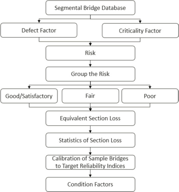
The condition factor is calculated based on both as-built conditions of the bridge and the most recent inspection notes. The following steps are recommended to find the condition factor. Section 6.5.10.4 offers an illustrative example.
- Step 1: Criticality factor (CF) is calculated for the bridge based on its as-built conditions. Table 6-58 shows various criteria for calculating CF and the score assigned. The bridge as-built plan is used to score the bridge for each criterion, then the total score is calculated. Simultaneously, summation of the maximums is calculated. When a criterion is not applicable (N/A), that criterion and its maximum are not considered. Finally, the total score is divided by the summation of the maximums to find CF. CF is calculated once and will not need to be updated in every inspection.
(6-52) where
CF = Criticality factor. Scorei = Score for every criterion (i = 1, 2, 3, . . . up to 19) in Table 6-58 that will be selected based on the bridge as-built plan. Max Scorei = Maximum score for every single criterion that was considered for the bridge. - Step 2: Defect factor (DF) is calculated for the bridge based on its most recent inspection notes. Table 6-59 shows various criteria for calculating defect factor and a score assigned. Bridge inspection notes are used to score the bridge for each criterion, then the total score is calculated. Simultaneously, summation of the maximums is calculated. Finally, the total score is divided by the summation of the maximums to find DF. For the practicality and consistency perspective, all criteria reflect the items in AASHTO’s Manual for Bridge Element Inspection (2019), except one additional type of defect that was observed in existing segmental bridge inspection reports. DF is recalculated in every inspection.
(6-53) where
DF = Defect factor. Scorej = Score for every single criterion (j = 1, 2, 3, . . . up to 7) in Table 6-59, which will be selected based on bridge inspection. Max Scorej = Maximum score for every criterion that was considered for the bridge.
The team reviewed the inspection reports of 87 segmental bridges in the database and summarized all the major types of deterioration/defects to create Table 6-59. The defects observed are in line with AASHTO’s Manual for Bridge Element Inspection (2019), which has been used in the bridge inspections, except for missing grout at segment joint or ungrouted/unfilled grout pocket. The team suggested incorporating missing grout at segment joint or ungrouted/unfilled grout pocket into the Manual for Bridge Element Inspection for segmental bridges because (1) it was observed in the inspections of a few segmental bridges and (2) large voids in longitudinal and transverse ducts were revealed after the collapse of a segmental post-tensioned bridge due to corrosion. The team discussed that large voids allowed corrosion at the joints to extend along the length of the tendon (Woodward 1989).
Table 6-58. Criticality factor (CF) adopted from FHWA-HIF-20-041.
| Criteria for Calculating Criticality Factor (CF) | Score | Rank | ||
| CF1: PT Tendon and Profile | Tendon Length | Tendon length < 100 ft | 0 | Low |
| Tendon length ≥ 100 ft to < 500 ft | 10 | Moderate | ||
| Tendon length ≥ 500 ft | 20 | High | ||
| Tendon Vertical Profile | Tendons with ≤ 24-in. profile | 0 | Low | |
| Tendons with > 24-in. and ≤ 6-ft profile | 20 | Moderate | ||
| Tendons with > 6-ft profile | 40 | High | ||
| Tendon Curvature | Straight tendons | 0 | Low | |
| Minimum radius of bending requirements met | 15 | Moderate | ||
| Minimum radius of bending requirements not met | 20 | High | ||
| Profile Conflict Avoidance | High level of detailing to avoid geometric conflicts, use of standard or proven designs | 0 | Low | |
| Limited or undesirable detailing | 15 | High | ||
| CF2: PT Tendon Joint and Closure | Cold Joints, Precast Segments | Continuous plastic duct or bridge without segmental joints | 0 | Low |
| Plastic ducts that include a duct coupler at joints | 10 | Moderate | ||
| Plastic ducts without duct coupling or metal ducts | 20 | High | ||
| Dry joints | N/A | Screen | ||
| Cold Joint, Cast-in-Place (CIP) Segments | Continuous plastic ducts or bridge without joints | 0 | Low | |
| Plastic ducts that include a duct coupler at joint | 7.5 | Moderate | ||
| Plastic ducts without duct coupling or metal ducts | 15 | High | ||
| Closure Pours | Adequate spacing for plastic duct couplers, recommended clearance, and resolving alignment | 0 | Low | |
| Adequate spacing for plastic duct couplers and recommended clearance, minimal spacing for alignment | 10 | Moderate | ||
| Inadequate spacing for plastic duct couplers and recommended clearance, or metal ducts of any design | 20 | High | ||
| CF3: PT System Materials and Components | Anchorage Protection, Interior | Four or more layers of protection | 0 | Low |
| Three layers of protection | 10 | Moderate | ||
| Two layers of protection | 20 | High | ||
| Inadequate drainage provided | N/A | Screen | ||
| Anchorage Protection, Exposed | Four layers of protection | 0 | Low | |
| Three layers of protection | 10 | Moderate | ||
| Less than three layers of protection | 20 | High | ||
| Venting | PTI/ASBI M50, PTI M55 PL-2 is specified | 0 | Low | |
| Protection | Venting other than deck, plastic ducts, and PTI/ASBI M50, PTI M55 PL-1 | 10 | Moderate | |
| Venting other than deck, metal ducts, and PTI/ASBI M50, PTI M55 PL-1 | 20 | High | ||
| Venting in deck and PTI/ASBI M50, PTI M55 PL-2 not specified | N/A | Screen | ||
| Grout Material Performance | Class C grout | 0; Internal 0; External | Low | |
| Class B grout | 10; Internal 15; External | Moderate | ||
| Class A grout | 20; Internal 30; External | High | ||
| Criteria for Calculating Criticality Factor (CF) | Score | Rank | ||
| Materials Specification | PTI/ASBI M50, PTI M55 specified for duct materials, handling of grout | 0 | Low | |
| PTI/ASBI M50, PTI M55 not specified for duct materials, handling of grout | 15 | High | ||
| Venting | Tendons with proper venting according to PTI/ASBI and all high points vented | 0 | Low | |
| External tendons with proper venting according to PTI/ASBI but high point not vented | 10 | Moderate | ||
| Improper or incomplete venting | 20 | High | ||
| Use of Diabolos | Diabolos with welded pipe connection | 0 | Low | |
| Diabolos with booted connection | 15 | Moderate | ||
| Diabolos not used | 20 | High | ||
| CF4: PT Installation Quality | Construction Quality | PTI/ASBI M50, PTI M55 specified and certified personnel used for operations, installation, grouting, and inspection | 0 | Low |
| PTI/ASBI M50, PTI M55 specified and certified personnel as direct supervisors of operations, installation, grouting, or inspection | 10 | Moderate | ||
| PTI/ASBI M50, PTI M55 not specified, without certified personnel for installation, grouting, and inspection | 20 | High | ||
| Quality Assurance | Effective QA to verify materials, records, installation, and personnel qualifications | 0 | Low | |
| Spot or random sampling, limited QA during construction | 7.5 | Moderate | ||
| Project relies only on QC process | 15 | High | ||
| Grouting Procedures | PTI/ASBI M50, PTI M55 procedures specified, pressure testing of ducts specified | 0 | Low | |
| PTI/ASBI M50, PTI M55 procedures specified, no pressure testing of ducts | 10 | Moderate | ||
| PTI/ASBI M50, PTI M55 not specified, no pressure testing of ducts | 20 | High | ||
| CF5: Environmental | Macro Environment | C-NA2 Other exterior exposure | 0 | Low |
| C-NA1 Interior exposure | ||||
| C-B Buried | ||||
| C-D1 Atmospheric in deicing salt environment | 20 | Moderate | ||
| C-D2 Indirect deicing salts | ||||
| C-M2 Marine submerged | ||||
| C-M1 Marine atmospheric | ||||
| C-D4 Direct deicing salt (High) | 40 | High | ||
| C-D3 Direct deicing (low) | ||||
| C-M3 Marine tidal/splash zone | ||||
| Micro or Local Environment | All other tendons | 0; A18 Moderate 0; A18 High | Low | |
| Tendons in plastic ducts located in the deck of a box girder or other exposed location | 10; A18 Moderate 20; A18 High | Moderate | ||
| Tendons in metal ducts located in the deck of a box girder or other exposed location | 15; A18 Moderate 30; A18 High | High | ||
Source: Washer (2022).
Table 6-59. Criteria for calculating defect factor (DF), adopted from AASHTO’s Manual for Bridge Element Inspection (2019) and identified by NCHRP Project 12-123.
| Criteria for Calculating Defect Factor (DF) | Score | Rank | Condition States | ||
| DF1 | Delamination/Patch Areas/Spalls | None | TBD | Low | CS1 |
| Delaminated. Spall 1 in. or less deep or 6 in. or less in diameter. Patched area that is sound. | TBD | Moderate | CS2 | ||
| Spall greater than 1-in. deep or greater than 6-in. diameter. Patched area that is unsound or showing distress. Does not warrant structural review. | TBD | High | CS3 | ||
| The condition warrants a structural review to determine the effect on strength or serviceability of the element or bridge; OR a structural review has been completed and the defects impact strength or serviceability of the element or bridge. | TBD | Very High | CS4 | ||
| DF2 | Exposed Rebars | None. | TBD | Low | CS1 |
| Present without measurable section loss. | TBD | Moderate | CS2 | ||
| Present with measurable section loss but does not warrant structural review. | TBD | High | CS3 | ||
| The condition warrants a structural review to determine the effect on strength or serviceability of the element or bridge; OR a structural review has been completed and the defects impact strength or serviceability of the element or bridge. | TBD | Very High | CS4 | ||
| DF3 | Exposed Prestressing | None. | TBD | Low | CS1 |
| Present without section loss. | TBD | Moderate | CS2 | ||
| Present with section loss but does not warrant structural review. | TBD | High | CS3 | ||
| The condition warrants a structural review to determine the effect on strength or serviceability of the element or bridge; OR a structural review has been completed and the defects impact strength or serviceability of the element or bridge. | TBD | Very High | CS4 | ||
| DF4 | Efflorescence/Rust Staining | None. | TBD | Low | CS1 |
| Surface white without build-up or leaching without rust staining. | TBD | Moderate | CS2 | ||
| Heavy build-up with rust staining. | TBD | High | CS3 | ||
| The condition warrants a structural review to determine the effect on strength or serviceability of the element or bridge; OR a structural review has been completed and the defects impact strength or serviceability of the element or bridge. | TBD | Very High | CS4 | ||
| DF5 | Cracks | Insignificant cracks or moderate-width cracks that have been sealed. Width less than 0.004 in. or spacing greater than 3 ft. | TBD | Low | CS1 |
| Unsealed moderate-width cracks or unsealed moderate pattern (map) cracking. Width 0.004–0.009 in. or spacing 1.0–3.0 ft. | TBD | Moderate | CS2 | ||
| Wide cracks or heavy pattern (map) cracking. Width greater than 0.009 in. or spacing less than 1 ft. | TBD | High | CS3 | ||
| The condition warrants a structural review to determine the effect on strength or serviceability of the element or bridge; OR a structural review has been completed and the defects impact strength or serviceability of the element or bridge. | TBD | Very High | CS4 | ||
| DF6 | Damage | Not applicable. | TBD | Low | CS1 |
| The element has impact damage. The specific damage caused by the impact has been captured in CS 2 under the appropriate material defect entry. | TBD | Moderate | CS2 | ||
| The element has impact damage. The specific damage caused by the impact has been captured in CS 3 under the appropriate material defect entry. | TBD | High | CS3 | ||
| The element has impact damage. The specific damage caused by the impact has been captured in CS 4 under the appropriate material defect entry. | TBD | Very High | CS4 | ||
| DF7 | Missing Grout at Segment Joint or Ungrouted/Unfilled Grout Pocket | None. | TBD | Low | CS1 |
| Present with ≤ 2 in.-deep area of missing grout/ungrouted or unfilled grout pocket. | TBD | Moderate | CS2 | ||
| Present with > 2-in.-deep area of missing grout/ungrouted or unfilled grout pocket. | TBD | High | CS3 | ||
| The condition warrants a structural review to determine the effect on strength or serviceability of the element or bridge; OR a structural review has been completed and the defects impact strength or serviceability of the element or bridge. | TBD | Very High | CS4 | ||
Table 6-60. Relation of risk and classes for selecting condition factor.
| Risk, % | Class for Selecting Condition Factor | Condition Factor |
|---|---|---|
| < 20 | Good/Satisfactory | 1.00 |
| 20 to 40 | Fair | 0.95 |
| > 40 | Poor | 0.85 |
- Step 3: Risk is calculated by the multiplication of CF and DF.
(6-54) where risk is corrosion risk of segmental superstructures as a percentage.
- Step 4: Find the condition factors from Table 6-60 based on the risk calculated in Step 3.
The three risk levels based on a 100-point risk scale proposed in FHWA-HIF-20-041 were used to relate condition classes with the risk. Table 6-60 shows the relation between the risk calculated by the proposed method and the classes for selecting the condition factor, as well as the condition factor. Bridge inspectors will use the condition factor, which is given in Table 6-60.
To determine the condition factors to use in the reliability analysis, the NCHRP Project 12-123 team proposed correlating the risk with the section loss of tendon based on the survey results. Table 6-61 shows the preliminary results of the relationship between the risk and the section loss of strands. Corrosion levels are based on the study by Franceschini et al. (2022). In Franceschini’s study, three levels of corrosion were defined as follows.
- The lower level of corrosion corresponds to a 2% strand unit-section loss.
- The medium corresponds to a 6% strand unit-section loss.
- The higher one corresponds to a 10% strand unit-section loss.
6.5.10.4 Illustrative Examples for ϕc
1. Simple Selection Method
| ϕc = 1.00 |
| ϕc = 1.00 |
| ϕc = 0.85 |
| ϕc = 0.90 |
Table 6-61. Relation of risk and section loss of strands.
| Risk, % | Class for Selecting Condition Factor | Section Loss of Strands, % |
|---|---|---|
| < 20 | Good/Satisfactory | 0 < SL < 2 |
| 20 to 40 | Fair | 2 ≤ SL < 6 |
| > 40 | Poor | 6 ≤ SL < 10 |
| ϕc = 1.00 |
| ϕc = 0.85 |
| ϕc = 0.90 |
| ϕc = 1.00 |
| ϕc = 0.85 |
For structures and conditions that fall between the previously described conditions, engineering judgment can be used to select an appropriate value for ϕc between 0.85 and 1.00.
If corrosion damage to bonded tendons is localized to a specific region or to one or more particular cross section, while the rest of the structure remains satisfactory, then the low value (0.85) may be applied to the damaged areas and a higher value to others. However, damage to an internal tendon at one section could indicate that it may be only partially effective at other sections, so caution is advised.
2. Alternative Approach
- Step 1: Calculation of CF.
Attribute Criteria for Calculating Criticality Factor (CF) Score Max CF1: PT Tendon and Profile Tendon Length Tendon length ≥100 to < 500 ft 10 20 Vertical Profile Tendons with > 6-ft profile 40 40 Tendon Curvature Straight tendons 0 20 Profile Conflict High level of detailing to avoid geometric conflicts, use of standard or proven designs 0 15 CF2: PT Tendon Joint and Closure Cold Joints (precast) Plastic ducts that include a duct coupler at joints 10 20 Cold Joints (CIP) Not applicable N/A 0 Closure Pours Adequate spacing for plastic duct couplers, recommended clearance, and resolving alignment 0 20 CF3: PT System Materials and Components Anchorage Protection, Interior Four or more layers of protection 0 20 Anchorage Protection, Exposed Four layers of protection 0 20 Venting Protection PTI/ASBI M50, PTI M55 PL-2 is specified 0 20 Grout Material Performance Class C grout 0 20
| Attribute | Criteria for Calculating Criticality Factor (CF) | Score | Max | |
| Materials Specification | PTI/ASBI M50, PTI M55 specified for duct materials, handling of grout | 0 | 15 | |
| Venting | Tendons with proper venting according to PTI/ASBI and all high points vented | 0 | 20 | |
| Use of Diabolos | Diabolos with welded pipe connection | 0 | 20 | |
| CF4: PT Installation Quality | Construction Quality | PTI/ASBI M50, PTI M55 specified and certified personnel used for operations, installation, grouting, and inspection | 0 | 20 |
| Quality Assurance | Effective QA to verify materials, records, installation, and personnel qualifications | 0 | 15 | |
| Grouting Procedures | PTI/ASBI M50, PTI M55 procedures specified, pressure testing of ducts specified | 0 | 20 | |
| CF5: Environmental | Macro Environment | C-D1 Atmospheric in deicing salt environment | 20 | 40 |
| Micro or Local Environment | All other tendons | 0 | 0 | |
| TOTAL | 80 | 365 | ||
| CF | 80/365 = 0.22 | |||
| Attribute | Criteria for Calculating Defect Factor (DF) | Score | Max | |
| DF1 | Delamination/Patch Areas/Spalls | Span 4 right web has 42-in. × 38.5-in. × 2.5-in.-deep spall and delamination. | 15 | 20 |
| DF2 | Exposed Rebars | None | 0 | 40 |
| DF3 | Exposed Prestressing | Corrosion to top post-tensioning tendon forward (towards the front side) of Pier 2 at the rubber boot.  |
10 | 50 |
| DF4 | Efflorescence/Rust Staining | Some patches at the segmental joints have light to moderate efflorescence | 5 | 20 |
| DF5 | Cracks | Some hairline cracks | 1 | 30 |
| DF6 | Damage | Not applicable. | 0 | 30 |
| DF7 | Missing Grout at Segment Joint or Ungrouted/Unfilled Grout Pocket | None | 0 | 40 |
| TOTAL | 31 | 230 | ||
| DF | 31/230 = 0.13 | |||


