CHAPTER 3
Crash Data Analysis and Findings

A crash data analysis was performed to investigate the effectiveness of delineation practices in reducing crash severity or crash frequency. The crash data analysis evaluated the two delineation practices identified in the previous chapter: mounting delineator panels on concrete barriers and mounting post-mounted delineators on guardrails. This chapter presents the methodology and findings for the crash data analysis of these two delineation practices.

Methodology

Site Selection

For each delineation practice, state DOTs were contacted to identify sites where the delineation practice was installed. Roadway information, such as annual average daily traffic, lane width, shoulder width, and the date of installation for the delineation practice, was also requested from state DOTs. If this information was unavailable, Google Maps was used to collect the information. Sites that installed the delineation practice of mounting delineator panels on concrete barriers were identified from California, Colorado, Texas, and Utah. Sites that installed the delineation practice of mounting post-mounted delineators on guardrails were identified from Michigan, Oregon, Pennsylvania, and Texas.

Data Collection

Once the sites were identified, crash data were collected and filtered at each site. The following filters were used to identify the following crashes of interest:

• First Harmful Event = Fixed Object
• Object Struck = Guardrail, Concrete Barrier, or Attenuation Device
• Distance = ± 1,000 ft

The delineator panels installed on concrete barriers can begin near a transition from a concrete barrier to a guardrail or near an attenuation device at the end of a concrete barrier. Thus, guardrails and attenuation devices were included in the object struck filter. The distance filter refers to searching for crashes within 1,000 ft of each end of the delineator panel installations. This filter helped capture crashes that may occur just beyond the beginning or end of the delineator panel installations, where the presence of delineation (or lack thereof) may still influence the driver because of visibility distance. The same filters were applied when crashes at the guardrail post-mounted delineator sites were searched for.

The collected and filtered crash data were grouped into four categories: (1) all lane departure (KABCO) crashes; (2) injury-related (e.g., fatal, incapacitating, and non-incapacitating injuries)

(KABC) crashes; (3) property-damage only (PDO) crashes; and (4) all crashes that occurred between 11 p.m. and 6 a.m. (defined as dark conditions in most crash datasets). The traffic flow variable was only available for some sites; none had traffic flow data for the before and after periods.

Analysis

A before-and-after study is usually used to estimate the effectiveness of a safety treatment. It is accomplished by first predicting the number of crashes at one or more sites where one or more treatments have been implemented during the after period if the treatment had not been implemented (π) and comparing that value with the expected number of crashes during the after period (λ) (i.e., after the implementation of the treatment) (Hauer 1997 and Lord et al. 2021). Common practice is to use a period of 3 years.

The effects of a treatment are estimated by comparing the two previously mentioned variables using the following equation:

(1)

If the number of crashes analyzed is below 500 for the before period, θ needs to be adjusted by the following factor: 1 + Var{π}/π². This adjustment minimizes the bias caused by a small sample size. The Index of Safety Effectiveness then becomes the following equation:

(2)

A value below 1.0 indicates a reduction in the number of crashes. To estimate the uncertainty associated with the Index of Safety Effectiveness, one needs to estimate the variance related to π and λ. The variable Var{π} is referred to as the variance of π, while the variable Var{λ} is referred to as the variance λ. The variance of the Index of Safety Effectiveness is equal to the following equation:

(3)

The safety effectiveness of an intervention is estimated using the following four-step process (Hauer 1997):

• Step 1: Estimate λ and π.
• Step 2: Calculate the variance of λ and π. As previously discussed, they are defined as Var{λ} and Var{π}, respectively.
• Step 3: Estimate θ.
• Step 4: Calculate the variance of θ. It is defined as Var{θ} in Equation 3.

In before-and-after studies, four general methods can be used to estimate the safety of a treatment: (1) the naïve or simple before-and-after study (Hauer 1997), (2) the before-and-after study with a reference group (Hauer 1997), (3) the before-and-after study using the EB method (Hauer 1997), and (4) the before-and-after study using the full Bayes method (Carlin and Louis 2008). The last three methods require data collection at reference sites (with characteristics similar to those of treatment sites where the treatment was not implemented). These methods

can account for changes that affect both the treated and non-treated sites (e.g., the economic conditions, weather conditions) similarly. In this research study, reference sites were unavailable for data collection and analysis. Thus, the simple before-and-after study approach was selected as the appropriate method.

For the simple before-and-after study, the crash data collected during the before period are used as the predicted value for the after period (π). With this method, the number of crashes can be adjusted for the differences in traffic flow and the length of the study period before and after the treatment is implemented. Equation 4 shows how the predicted value can be adjusted as a function of traffic flow and periods (Hauer 1997):

(4)

where

π̂	=	the predicted number of crashes for the after period,
rd	=	(or the ratio between the after and before periods),
rtf	=	(or the ratio in traffic flow between the after and before periods), and
	=	the estimated number of crashes during the before period (in this case, the number of crashes during the before period).

The “^” in Equation 4 and all subsequent equations refers to an estimate of a variable. The ratio r_tf can be linear or nonlinear, , depending on the characteristics of the data. Usually, β has been shown to vary between 0.5 and 1.0 (the latter representing a linear relationship). The variances for the simple method are defined as follows:

(5)

(6)

In Equation 5, the uncertainty associated with r_tf was not included in the variance calculation since the traffic flow coefficient of variation was unknown. The variance of λ is equal to the number of crashes during the after period, assuming that the crash count follows a Poisson distribution over the entire study period.

Although the simple before-and-after method is straightforward and easy to use, it is limited in that:

• It does not account for local and regional changes, such as weather patterns and economic conditions; and
• It does not account for the regression-to-the-mean (RTM) and site selection effects.

The RTM dictates that sites characterized by a large (or small) number of observations during the before period are expected to observe a smaller (or larger) number of observations during the after period, closer to the long-term average or mean of the site, if nothing changes. Site selection effects refer to sites where an entry criterion is used to select sites for further analyses (e.g., a minimum of four crashes per year). Although both biases are related, they do differ (Lord and Kuo 2012; Lord et al. 2021).

Findings

The following two sections present findings from the crash data analysis of the concrete barrier delineator panel and guardrail post-mounted delineator delineation practices using the methodology previously discussed.

Concrete Barrier – Delineator Panels

The various sites with delineator panels installed on concrete barriers were identified and compiled from California, Colorado, Texas, and Utah. A total of 65 sites with delineator panel installations were identified from these four states. Some of these sites had multiple installations (e.g., northbound and southbound directions at an interchange) or long roadway segments with the installation. In California, the delineator panel sites were located at an interchange with overpasses and a few tunnels. Similarly, in Texas, delineator panels had been installed at several interchange and overpass locations in the Dallas region. In Colorado and Utah, delineator panels had been installed at several curved roadway segments. Crashes were categorized into four categories: (1) KABCO, (2) KABC, (3) PDO, and (4) dark conditions. A period of 3 years was used to evaluate crashes that occurred 3 years before installation and 3 years after installation.

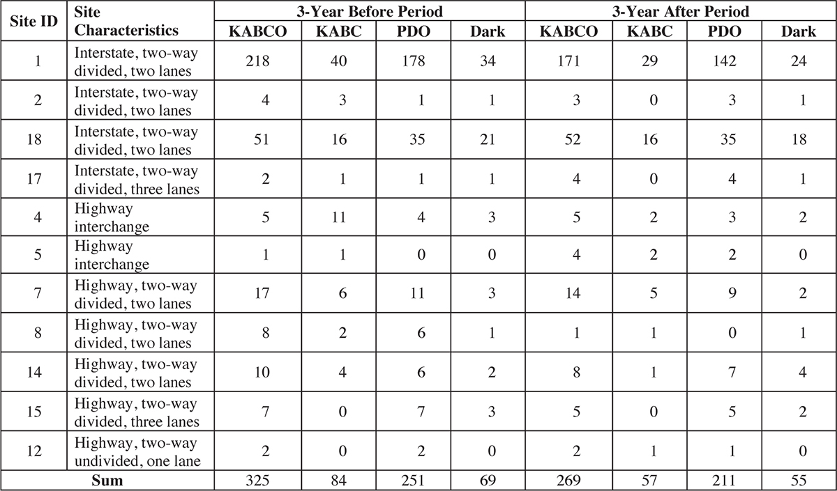
Table 4 summarizes the statistics for the data collected in California. The crashes that met the applicable filters occurred at five sites. Fourteen crashes occurred 3 years before installation, and seven crashes occurred 3 years after installation. Table 5 summarizes the statistics for the data collected in Colorado. The crashes that met the applicable filters occurred at 11 sites. Three hundred and twenty-five crashes occurred 3 years before installation, and 269 crashes occurred 3 years after installation.

After the filters were applied to the crash data collected in Texas, no applicable crashes were identified at the sites with delineator panels installed on concrete barriers. Thus, no data for Texas are presented in this section. Table 6 summarizes the statistics for the data collected in Utah. The crashes that met the applicable filters occurred at five sites. Nine crashes occurred 3 years before installation, and 12 crashes occurred 3 years after installation.

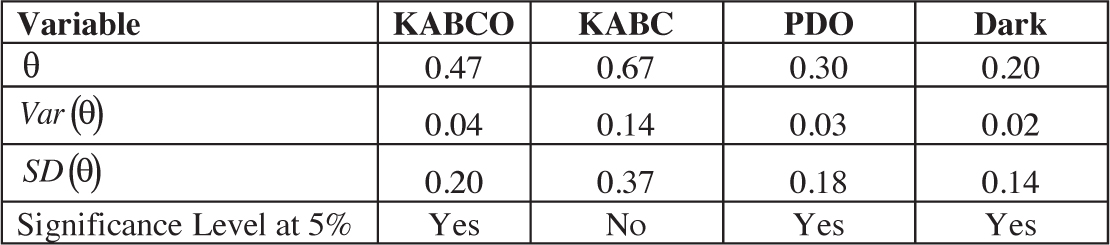
Tables 7 through 9 show the results of the simple before-and-after analysis of the crashes that occurred in California, Colorado, and Utah. The tables also show the Index of Safety Effectiveness (θ), its variance (Var(θ)), standard deviation (SD(θ)), and significance level. A value below 1 for the Index of Safety Effectiveness indicates a reduction in crashes. The 95% confidence interval (θ ± 1.96 * SD(θ)) was calculated to determine whether the crash reduction was statistically significant. If the value of 1 was not within the 95% confidence interval range, the reduction in crashes was considered statistically significant at a 5% level. As such, this result indicates strong evidence that the reduction in crashes is not because of random variation.

Long Description.

The table displays four columns and six rows, where the last row shows the total sum for the last two columns. The column headers are Site ID, Site Characteristics, 3-Year Before Period, and 3-Year After Period. The third and fourth columns are divided into four sub-columns as follows: KABCO, KABC, PDO, and Dark. The data provided row-wise are as follows:

2; Tunnel; 2; 0; 2; 2; 0; 0; 0; 0

6; Highway interchange; 4; 2; 2; 2; 4; 1; 3; 1

7; Highway interchange; 3; 2; 1; 1; 0; 0; 0; 0

8; Highway interchange; 0; 0; 0; 0; 2; 2; 0; 0

9; Highway interchange; 5; 1; 4; 4; 1; 1; 0; 1

Sum; 14; 5; 9; 9; 7; 4; 3; 2

Long Description.

The table displays four columns and 12 rows, where the last row shows the total sum for the last two columns. The column headers are Site ID, Site Characteristics, 3-Year Before Period, and 3-Year After Period. The third and fourth columns are divided into four sub-columns as follows: KABCO, KABC, PDO, and Dark. The data provided row-wise are as follows:

1; Interstate, two-way divided, two lanes; 218; 40; 178; 34; 171; 29; 142; 24

2; Interstate, two-way divided, two lanes; 4; 3; 1; 1; 3; 0; 3; 1

18; Interstate, two-way divided, two lanes; 51; 16; 35; 21; 52; 16; 35; 18

17; Interstate, two-way divided, three lanes; 2; 1; 1; 1; 4; 0; 4; 1

4; Highway interchange; 5; 11; 4; 3; 5; 2; 3; 2

5; Highway interchange; 1; 1; 0; 0; 4; 2; 2; 0

7; Highway, two-way divided, two lanes; 17; 6; 11; 3; 14; 5; 9; 2

8; Highway, two-way divided, two lanes; 8; 2; 6; 1; 1; 1; 0; 1

14; Highway, two-way divided, two lanes; 10; 4; 6; 2; 8; 1; 7; 4

15; Highway, two-way divided, three lanes; 7; 0; 7; 3; 5; 0; 5; 2

12; Highway, two-way undivided, one lane; 2; 0; 2; 0; 2; 1; 1; 0

Sum: 325; 84; 251; 69; 269; 57; 211; 55

Long Description.

The table displays four columns and six rows, where the last row shows the total sum for the last two columns. The column headers are Site ID, Site Characteristics, 3-Year Before Period, and 3-Year After Period. The third and fourth columns are divided into four sub-columns as follows: KABCO, KABC, PDO, and Dark. The data provided row-wise are as follows:

6; Divided highway, two lanes; 3; 1; 2; 0; 3; 0; 3; 1

7; Divided highway, two lanes; 1; 0; 1; 0; 4; 1; 3; 0

11; Divided highway, two lanes; 0; 0; 0; 0; 1; 0; 1; 1

12; Divided highway, two lanes; 4; 0; 4; 2; 3; 1; 2; 0

14; Divided highway, two lanes; 1; 1; 0; 0; 1; 0; 0; 0

Sum; 9; 2; 7; 2; 12; 2; 9; 2

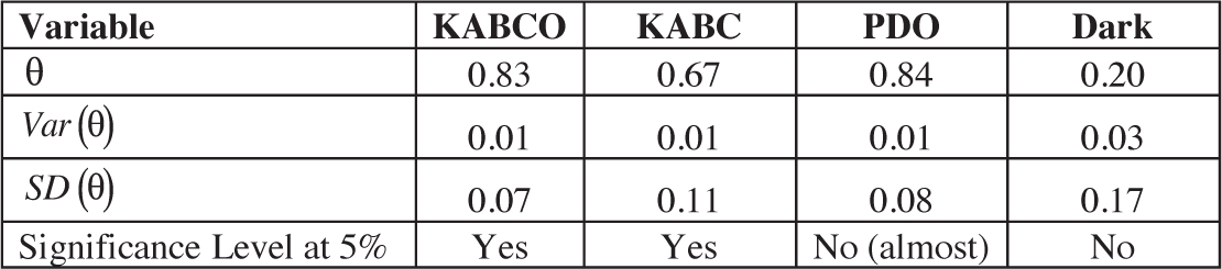
Table 7 shows that a reduction in crashes was observed for all categories, although the reduction in injuries was not statistically significant. Table 8 also shows that a reduction in crashes was observed for all categories, although the reductions in PDO and dark conditions crashes were not statistically significant.

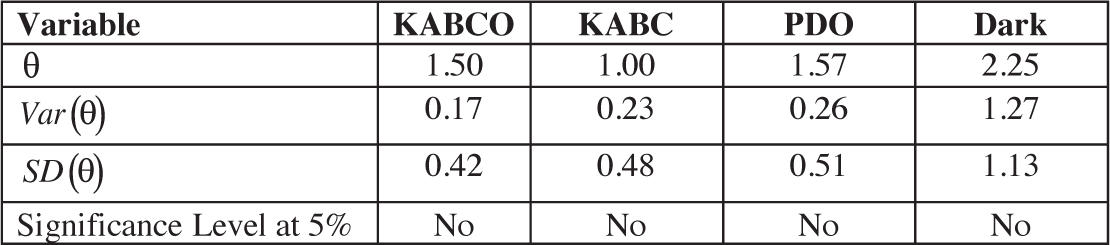
Overall, the reductions observed for Colorado and Utah were smaller than those observed for California. Colorado benefited from a larger crash dataset. Table 9 shows that no reduction in

Long Description.

The table shows five columns and four rows. The column headers are Variable, KABCO, KABC, PDO, and Dark. The data provided row-wise are as follows:

Index of Safety Effectiveness; 0.47; 0.67; 0.30; 0.20

Variance; 0.04; 0.14; 0.03; 0.02

Standard Deviation; 0.20; 0.37; 0.18; 0.14

Significance Level at 5%; Yes; No; Yes; Yes

Long Description.

The table shows five columns and four rows. The column headers are Variable, KABCO, KABC, PDO, and Dark. The data provided row-wise are as follows:

Index of Safety Effectiveness; 0.83; 0.67; 0.84; 0.20

Variance; 0.01; 0.01; 0.01; 0.03

Standard Deviation; 0.07; 0.11; 0.08; 0.17

Significance Level at 5%; Yes; Yes; No (almost); No

Long Description.

The table shows five columns and four rows. The column headers are Variable, KABCO, KABC, PDO, and Dark. The data provided row-wise are as follows:

Index of Safety Effectiveness; 1.50; 1.00; 1.57; 2.25

Variance; 0.17; 0.23; 0.26; 1.27

Standard Deviation; 0.42; 0.48; 0.51; 1.13

Significance Level at 5%: No; No; No; No

crashes was observed for all categories. The Utah-analyzed dataset was small and thus subject to greater effects from randomness. Utah was also one of the sites that required estimation of the installation date using Google Maps. Error likely occurred in the estimation of these data, resulting in the incorrect identification of crashes that occurred before installation as crashes that occurred after installation and vice versa.

Guardrail – Post-Mounted Delineators

The various sites with post-mounted delineators installed on guardrails were identified and compiled from Michigan, Oregon, Pennsylvania, and Texas. A total of 37 sites with post-mounted delineator installations were identified from these four states. Some of these sites had multiple installations (i.e., on both sides of the roadway) or long roadway segments with the installation. Crashes were categorized into four categories: (1) KABCO, (2) KABC, (3) PDO, and (4) dark conditions. A period of 3 years was used to evaluate crashes that occurred 3 years before installation and 3 years after installation.

Table 10 summarizes the statistics for the data collected in Michigan. The crashes that met the applicable filters occurred at 11 sites. Two hundred and twenty-three crashes occurred 3 years before installation, and 127 crashes occurred 3 years after installation.

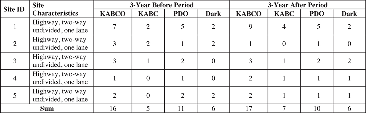
Table 11 summarizes the statistics for the data collected in Oregon. The crashes that met the applicable filters occurred at 11 sites. Nine crashes occurred 3 years before installation, and six crashes occurred 3 years after installation. Table 12 summarizes the statistics for the data collected in Pennsylvania. The crashes that met the applicable filters occurred at 10 sites. Sixty-three crashes occurred 3 years before installation, and 41 crashes occurred 3 years after installation. Table 13 summarizes the statistics for the data collected in Texas. The crashes that met the applicable filters occurred at five sites. Sixteen crashes occurred 3 years before installation, and 17 crashes occurred 3 years after installation.

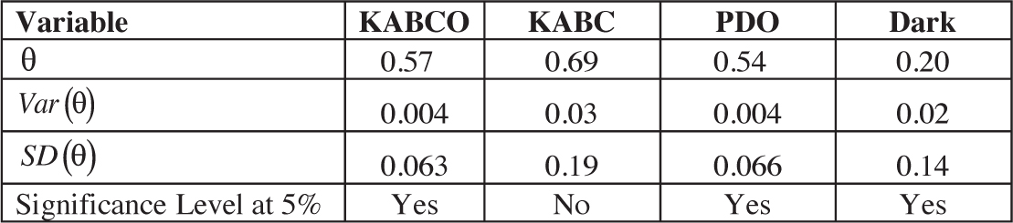
Tables 14 through 17 show the results of the simple before-and-after analysis of the crashes that occurred in Michigan, Oregon, Pennsylvania, and Texas. The tables show the Index of Safety Effectiveness (θ), its variance (Var(θ)), standard deviation (SD(θ)), and significance level. A value below 1 for the Index of Safety Effectiveness indicates a reduction in crashes.

Long Description.

The table displays four columns and six rows, where the last row shows the sum for the two columns. The column headers are Site ID, Site Characteristics, 3-Year Before Period, and 3-Year After Period. The third and fourth columns are divided into four sub-columns as follows: KABCO, KABC, PDO, and Dark. The data provided row-wise are as follows:

1; Highway, two-way undivided, one lane; 7; 2; 5; 2; 9; 4; 5; 2

2; Highway, two-way undivided, one lane; 3; 2; 1; 2; 1; 0; 1; 0

3; Highway, two-way undivided, one lane; 3; 1; 2; 0; 3; 1; 2; 2

4; Highway, two-way undivided, one lane; 1; 0; 1; 0; 2; 1; 1; 1

5; Highway, two-way undivided, one lane; 2; 0; 2; 2; 2; 1; 1; 1

Sum; 16; 5; 11; 6; 17; 7; 10; 6

The 95% confidence interval (θ ± 1.96 ✽ SD(θ)) was calculated to determine whether the crash reduction was statistically significant. If the value of 1 was not within the 95% confidence interval range, then the reduction in crashes was considered statistically significant at a 5% level. As such, this result indicates strong evidence that the reduction in crashes was not because of random variation.

Table 14 shows that a reduction in crashes was observed for all categories, although the reduction in injuries was not statistically significant. Michigan benefited from a larger analyzed crash dataset. Table 15 also shows that a reduction in crashes was observed for all categories except for dark conditions. However, the reduction in crashes for KABCO and PDO was not statistically significant because of the small sample size. Table 16 shows that a reduction in crashes was observed for all categories. However, the reduction in crashes for KABC and dark conditions was not statistically significant because of the small sample size. Table 17 shows that

Long Description.

The table shows five columns and four rows. The column headers are Variable, KABCO, KABC, PDO, and Dark. The data provided row-wise are as follows:

Row 1: Index of Safety Effectiveness; 0.57; 0.69, 0.54, 0.20

Row 2: Variance; 0.004; 0.03; 0.004; 0.02

Row 3: Standard Deviation; 0.063; 0.19; 0.066; 0.14

Row 4: Significance Level at 5%; Yes; No; Yes; Yes

Long Description.

The table shows five columns and four rows. The column headers are Variable, KABCO, KABC, PDO, and Dark. The data provided row-wise are as follows:

Row 1: Index of Safety Effectiveness; 0.60; 0.25, 0.71, 1.00

Row 2: Variance; 0.08; 0.05; 0.14; 0.33

Row 3: Standard Deviation; 0.28; 0.22; 0.37; 0.57

Row 4: Significance Level at 5%; No; Yes; No; No

Long Description.

The table shows five columns and four rows. The column headers are Variable, KABCO, KABC, PDO, and Dark. The data provided row-wise are as follows:

Row 1: Index of Safety Effectiveness; 0.64; 0.71, 0.59, 0.81

Row 2: Variance; 0.02; 0.05; 0.02; 0.06

Row 3: Standard Deviation; 0.13; 0.23; 0.14; 0.25

Row 4: Significance Level at 5%; Yes; No; Yes; No

Long Description.

The table shows five columns and four rows. The column headers are Variable, KABCO, KABC, PDO, and Dark. The data provided row-wise are as follows:

Row 1: Index of Safety Effectiveness; 0.64; 0.71, 0.59, 0.81

Row 2: Variance; 0.11; 0.32; 0.11; 0.18

Row 3: Standard Deviation; 0.33; 0.23; 0.33; 0.42

Row 4: Significance Level at 5%; No; No; No; No

a reduction in crashes was only observed for PDO. The crash dataset for Texas was limited to a small sample size.

Discussion

A simple before-and-after analysis was used to analyze the crash data collected at various sites with delineation practices. A more detailed analysis approach, such as including a reference group or applying the EB method (Hauer 1997), could not be used because of the limited sample size and lack of detailed site-specific roadway information and traffic patterns. Two delineation practices were evaluated using the simple before-and-after analysis approach: (1) installing delineator panels on concrete barriers and (2) installing post-mounted delineators on guardrails.

The simple before-and-after analysis indicated a statistically significant reduction in KABCO crashes in Colorado at sites with delineator panels installed on concrete barriers. California and Utah had significantly small data sizes (i.e., fewer than 20 crashes). As such, they typically did not indicate a statistically significant reduction in crashes because of small sample sizes and randomness. Although the analysis was limited to findings from a single state, a positive safety effect was observed for delineator panels installed on concrete barrier systems. A statistically significant reduction in crashes was observed for sites with post-mounted delineators installed on guardrail systems in Michigan and Pennsylvania.

An overall reduction in crashes was not observed for sites with post-mounted delineators installed on guardrail systems in Oregon and Texas. However, these datasets were limited in their analysis because of a significantly small sample size (i.e., fewer than 20 crashes). An additional limitation in analyzing the safety effect of the guardrail post-mounted delineators was the influence of other safety improvements often included when installing these delineation practices. For example, installing post-mounted delineators at some guardrail sites was accompanied by repaving the roadway, which increases surface friction and lowers the chance of a vehicle departing the travel lane. As a result, it was challenging to identify which roadway or roadside improvement contributed to the reduction in crashes. This limitation was observed for all the installation sites with guardrail post-mounted delineators, except for the Michigan sites. Installing post-mounted delineators on guardrail systems at the Michigan sites was the only safety improvement. Overall, installing post-mounted delineators adjacent to the traveled way seems to produce a positive effect on safety.

Summary

A crash data analysis evaluated the effect of installing two different delineation practices on longitudinal roadside hardware. The first practice consisted of installing delineator panels on concrete barriers; the second practice consisted of installing post-mounted delineators on guardrails. Sites with delineator panels installed on concrete barriers were identified from California, Colorado, Texas, and Utah. Sites with post-mounted delineators installed on guardrails were

collected from Michigan, Oregon, Pennsylvania, and Texas. The analysis methodology consisted of a simple before-and-after approach.

The installation of delineator panels on concrete barriers and post-mounted delineators on guardrails indicated a reduction in KABCO, KABC, PDO, and dark conditions crashes. However, the magnitude of the reduction could have been influenced by other countermeasures implemented at the same site, such as repaving the roadway surface. Despite the limitations of the simple before-and-after study, the safety trend seems positive after the installation of the delineator panels and post-mounted delineators.